The kinematical structure of gravitationally lensed arcs

Abstract

In this paper the expected properties of the velocity fields of strongly lensed arcs behind galaxy clusters are investigated. The velocity profile along typical lensed arcs is determined by ray tracing light rays from a model source galaxy through parametric cluster toy-models consisting of individual galaxies embedded in a dark cluster halo. We find that strongly lensed arcs of high redshift galaxies show complex velocity structures that are sensitive to the details of the mass distribution within the cluster, in particular at small scales. From fits to the simulated imaging and kinematic data we demonstrate that reconstruction of the source velocity field is in principle feasible: two dimensional kinematic information obtained with Integral Field Units (IFU’s) on large ground based telescopes in combination with adaptive optics will allow the reconstruction of rotation curves of lensed high redshift galaxies. This makes it possible to determine the mass-to-light ratios of galaxies at redshifts $z>~{}1$ out to about 2-3 scale lengths with better than $\sim 20\%$ accuracy. We also discuss the possibilities of using two dimensional kinematic information along the arcs to give additional constraints on the cluster lens mass models.

1 Introduction

In recent years, the high redshift universe has become a focus of attention for observational cosmology as a testbed for theoretical models of galaxy formation and cosmology. The detection of high redshift galaxies and quasars has led to the first observational tests of reionisation models (Haiman & Holder, 2003; Ciardi & Ferrara, 2005) and high redshift absorption line systems have helped to constrain spin temperatures and the fraction of cold neutral gas in high redshift galaxies (Kanekar & Chengalur, 2003). Source counts in the sub-mm and the infrared have constrained the star formation at high redshifts (Hughes et al., 1998; Blain et al., 1999). However, despite these tremendous advances in the field, a few questions pertaining to the high redshift universe and the evolution of galaxies remain difficult to address. Foremost, there is the open question as to the role of the dark matter in galaxy evolution. Even in the local universe, the presence of dark matter can only be inferred indirectly through its gravitational effect; for example by measuring the rotation curves of galaxies.

Rotation curves have now been measured for a large sample of nearby galaxies, both in optical wavelengths (Mathewson et al., 1992; Persic & Salucci, 1995; Palunas & Williams, 2000) and using the 21cm emission line of neutral hydrogen (Verheijen & Sancisi, 2001; Swaters, 1999). They have improved our knowledge of the systematics of dark matter in nearby galaxies, but they have also led to a number of new questions that still need to be addressed in theoretical models of galaxy formation. The strong dependence of rotation curve shape and amplitude on the optical luminosity indicates a tight coupling between luminous and dark matter that is not expected from the current models (Persic et al., 1996; Donato et al., 2004). There are also indications from the rotation curves of low surface brightness galaxies that galactic dark matter haloes contain a constant density core, as opposed to the $r^{-1}$ cusp predicted by simulations (de Blok et al., 2001; de Blok & Bosma, 2002).

Using $H\alpha$ emission, rotation curves of galaxies have been measured accurately up to redshifts of about $0.3$. $H\alpha$ emission has been detected out to much larger distances and has been used to constrain the star formation rates in galaxies at redshifts greater than 2 (Bunker et al., 1999). Attempts have also been made to measure the rotation curves of galaxies up to redshifts of $z\sim 1$ (Vogt et al., 1996; Vogt et al., 1997; Hudson et al., 1998; Böhm et al., 2004), but at these redshifts it is difficult to determine the inclination angle of the rotating disc accurately and to obtain sufficient spatial resolution. So far the limited spatial resolution has only allowed determinations of the total velocity dispersion rather than actual rotation curves: therefore most authors concentrated on constraining the evolution of the Tully-Fisher relation (Tully & Fisher, 1977).

Galaxies that are at a higher redshift but are strongly lensed may well be magnified by factors of 10 or more (e.g. Blandford & Narayan, 1992). Exploiting this effect, gravitational lensing has already been successfully used as a tool to study high redshift sources in greater detail than would be otherwise possible (Pelló et al., 1999; Ellis et al., 2001; Richard et al., 2003). Lensed galaxies may have a large enough area and luminosity to make a measurement of their rotation curve possible, despite their larger distance. Narasimha & Chitre (1993) demonstrated that it is in principle possible to measure the kinematics of galaxies that are much more distant in this way. Since integral field spectrometers had not been developed at the time of the publication of that paper, it focused on measuring the velocities along straight arcs. Long slit spectroscopy of straight arcs has been carried out successfully by Bunker et al. (2000) and Mehlert et al. (2001). Recently, improvements in resolution and sensitivity of integral field spectrometers have made it possible to obtain kinematics of moderately magnified background galaxies (Swinbank et al., 2003).

At intermediate redshifts between $z\sim 0.3-1$, gravitational lensing also provides constraints on the dark matter content of the inner $10-200\,\mathrm{kpc}$ of lens galaxies (e.g. Koopmans et al., 1998; Koopmans & Treu, 2003) and lens clusters (e.g. Smail & Dickinson, 1995; Mellier, 1999; Kneib et al., 2003). Determinations of the dark matter distribution using gravitational lensing rely on accurate data to provide sufficient constraints on the lens mass model. Degeneracies in the lens model usually exist and may have important consequences for determinations of cosmological parameters and mass density profiles from lensing (Williams et al., 1999; Zhao & Qin, 2003; Meneghetti et al., 2004; Dalal et al., 2004). Additional constraints help to break such degeneracies. For galaxy lenses, spectroscopic studies have been used to break degeneracies in the lens models and constrain their mass distribution further (Koopmans & Treu, 2002).

In this paper we investigate the possibilities of measuring rotation curves of lensed galaxies with current and upcoming instruments and discuss the additional constraints on the foreground lens mass model that may be obtained from two dimensional spectroscopic data.

We begin by describing the theoretical framework, the ray-tracing method and the source and cluster lens models in § 2. In § 3 we briefly discuss the optical properties of known lensed arcs. In § 4 we present the kinematics of simulated arcs and discuss their generic properties. In § 5 we discuss how the kinematic profile of the source can be reconstructed from lens modeling and discuss their dependence on the lens mass model. We address the observational possibilities using current and future instruments – in particular the use of Integral Field Units (IFUs) – in § 6. We conclude with a discussion and summary in § 7.

Throughout this paper we use a standard $\Lambda$CDM cosmology with $\Omega_{\Lambda}=0.7$, $\Omega_{\mathrm{m}}=0.3$ and $H_{0}=70\,\mathrm{km\,s^{-1}\,Mpc^{-1}}$.

2 Simulating data cubes of lensed high redshift galaxies

2.1 Lensing theory

A background source at a redshift $z_{\mathrm{s}}$ that is located at a position $\mathbf{\beta}$ will appear at a position $\mathbf{\theta}$ on the sky if it is lensed by a massive foreground object at redshift $z_{\mathrm{l}}$ so that

$$\mathbf{\theta}=\mathbf{\beta}+\frac{D_{\mathrm{LS}}}{D_{\mathrm{OS}}}\alpha(\mathbf{\theta}),$$ (1)

where $D_{\mathrm{LS}}$ and $D_{\mathrm{OS}}$ are the angular diameter distances from lens to source and from observer to source, respectively. The deflection angle $\mathbf{\alpha}$ at position $\mathbf{\theta}$ on the lens plane is given by

$$\mathbf{\alpha}(\mathbf{\theta})=\frac{D_{\mathrm{OS}}}{\pi D_{\mathrm{LS}}}\int\kappa(\mathbf{\theta^{\prime}})\frac{\mathbf{\theta}-\mathbf{\theta^{\prime}}}{\left|\mathbf{\theta}-\mathbf{\theta^{\prime}}\right|^{2}}\,d^{2}\theta^{\prime},$$ (2)

where $\kappa$ is a dimensionless quantity related to the surface mass density $\Sigma$ through,

$$\kappa(\mathbf{\theta})=\Sigma(\mathbf{\theta})\times\frac{4\pi GD_{\mathrm{OL}}D_{\mathrm{LS}}}{c^{2}D_{\mathrm{OS}}}.$$ (3)

The magnification of an image at position $\theta$ of a point source at position $\beta$ is given by

$$\mu(\mathbf{\theta})=\frac{1}{[1-\kappa(\mathbf{\theta})]^{2}-\gamma^{2}(\mathbf{\theta})},$$ (4)

where $\mathbf{\gamma}=(\gamma_{x},\gamma_{y})$ is the total shear at the image position, which is related to the deflection angle, and hence the lensing mass distribution, through:

$$\gamma_{x} = \frac{1}{2}\left(\frac{\partial\alpha_{x}}{\partial x}-\frac{\partial\alpha_{y}}{\partial y}\right),$$ (5)

$$\gamma_{y} = \frac{\partial\alpha_{y}}{\partial x}=\frac{\partial\alpha_{x}}{\partial y}.$$ (6)

For extended sources, different parts of the source will be magnified by different amounts, leading to differential magnification (Blain, 1999). Given a magnification map on the source plane $\mu_{\mathrm{s}}(\mathbf{\beta})$ and the source flux $F_{\mathrm{s}}(\mathbf{\beta})$, the observed total flux is

$$F_{\mathrm{tot}}=\int F_{\mathrm{s}}(\mathbf{\beta})\mu_{\mathrm{s}}(\mathbf{\beta})\,d^{2}\beta.$$ (7)

The type of observations we are interested in here, namely spatial spectroscopy using integral field units, are characterised by several channels at frequencies $\nu$, of bandwidth $\Delta\nu$. The observed flux in an interval between $\nu$ and $\nu+d\nu$ would be

$$F(\nu)\,d\nu=\int F_{\mathrm{s}}(\nu,\mathbf{\beta})\mu_{\mathrm{s}}\left(\mathbf{\beta}\right)\,d^{2}\beta d\nu,$$ (8)

and so, for finite bandwidths,

$$F(\nu)=\int_{\nu}^{\nu+\Delta\nu}\!\!\!\int F_{\mathrm{s}}\left(\nu,\mathbf{\beta}\right)\mu_{\mathrm{s}}\left(\mathbf{\beta}\right)\,d^{2}\beta d\nu.$$ (9)

Thus, if $\mu_{\mathrm{s}}\left(\mathbf{\beta}\right)$ is known from the lens model, it is straightforward to obtain the total observed flux at a given wavelength, given a model of the source. This can be done simply by summing over all the pixels of a map that is the product of the source flux at the observed wavelength and the source magnification map.

2.2 Modeling the source and creating mock kinematic data

In order to create a model data cube for the source, we need to make assumptions about the gas distribution and its kinematics.

For the latter, we take the ‘Universal Rotation Curve’ as derived by Persic et al. (1996). We assume an $L_{*}$ galaxy, for which their equations reduce to:

$$V^{*}(x)=V_{0}^{*}\sqrt{\frac{1.4x^{1.2}}{(x^{2}+0.6)^{1.4}}+\frac{1.1x^{2}}{x^{2}+2.2}},$$ (10)

with $x=R/R_{\mathrm{opt}}=R/3.2h$ being the radius expressed in units of $R_{\mathrm{opt}}$, which is the radius encompassing $83\%$ of the total light; $h$ is the disc scale length. We set the parameter $V_{0}^{*}=201.5\,\mathrm{km/s}$. Defining the radius expressed in disc scale lengths, $x_{\mathrm{h}}=R/h$, we get:

$$V^{*}(x_{\mathrm{h}})=V_{0}^{*}\sqrt{\frac{0.3x_{\mathrm{h}}^{1.2}}{(0.1x_{\mathrm{h}}^{2}+0.6)^{1.4}}+\frac{0.1x_{\mathrm{h}}^{2}}{0.1x_{\mathrm{h}}^{2}+2.2}}.$$ (11)

In reality, galaxies do not follow the Universal Rotation Curve exactly, and galaxies with different masses will have different shapes for their rotation curves. Furthermore, Persic et al. (1996) derived their equations from rotation curves of galaxies in the local universe, and their results may not be directly applicable to the high-redshift galaxies we are studying here. However, the exact shape and amplitude of the rotation curve is not critical for the study we present here and different assumptions would not affect our conclusions.

For the gas distribution, we assume an exponential radial profile:

$$I=I_{0}\exp(-x_{\mathrm{h}}).$$ (12)

We adopt a radial scale-length of $h=0.4$ arcsec, corresponding to approximately 4 kpc at the assumed source redshift of $z_{\mathrm{s}}=1.5$. Furthermore we assume that the disc of the galaxy is inclined at an angle of 50 degrees with respect to the line of sight. The vertical density distribution of the gas is assumed to be exponential as well, with scale-height ${\mathrm{z}_{0}}$ equal to 1/20th of the radial scale-length $h$. This means we effectively assume the galaxy to be razor thin, but the effect of a larger vertical scale-height on the simulated data cube is very small for the moderate inclination of 50 degrees we assume here.

To create the model data cube, we use the GALMOD task in GIPSY: The Groningen Image Processing SYstem. It uses a Monte-Carlo integration to fill the model galaxy with small gas clouds, following the exponential distribution given above. For each cloud, the radial velocity is calculated on the basis of its position in the disc and the rotation velocity at its radius, and each cloud is assumed to emit a gaussian emission line with an intrinsic velocity width of $10\,{\mathrm{km/s}}$. The final data cube consists of channel-maps spaced $\approx 8\,{\mathrm{km/s}}$, with spatial pixels of $0.02$ arcsec, or $h/20$.

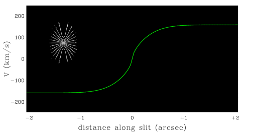
Figure 1: Position-velocity diagram of the source along the major axis. Contours correspond to the maximum intensities at 1, 3 and 5 radial scale lengths. The green line indicates the rotation curve, multiplied by $\sin(50^{\circ})$. The inset in the top left shows the velocity map of the source. The distances along the axes are in arcseconds. Different colours indicate radial velocities, ranging from -175 to 175 $\,{\mathrm{km/s}}$, as indicated by the colour bar; the contours range from -150 to 150$\,{\mathrm{km/s}}$ with intervals of $25\,{\mathrm{km/s}}$.

In Fig. 1, we show a cut through the data cube along the major axis of the galaxy.

From the data cube, we derive an image of the integrated gas emission by adding up, at each pixel position, the signal in the individual channel maps. The velocity field is derived by fitting gaussians to the line profiles. It is shown in the inset in Fig. 1, and resembles those observed in nearby spiral galaxies (Verheijen & Sancisi, 2001; Garrido et al., 2002).

In the first instance, we use a very high number of small gas clouds in the Monte-Carlo integration. This results in a very smooth gas distribution and velocity field. We can simulate a very patchy gas distribution by limiting the number of clouds to a very small number. We will discuss how such strong substructure in the source will affect our results in § 4.2 and § 5.5.

2.3 Modeling the lensing potential

Simulations of strongly lensed arcs in clusters have been performed by several groups (Bartelmann & Weiss, 1994; Wu & Mao, 1996; Hamana & Futamase, 1997; Bartelmann et al., 1998; Wambsganss et al., 1998; Meneghetti et al., 2001; Meneghetti et al., 2003). Most of these studies make use of a cluster model from N-body simulations. In contrast, the basic approach in our work is to use an analytic, parametric cluster model. Analytic models have been used to predict the arc statistics for different cosmologies by Wu & Mao (1996), Cooray (1999) and Oguri et al. (2001), finding a much lower cross section for the formation of arcs than when clusters are modeled directly from N-body simulations. As pointed out by Meneghetti et al. (2003) massive cluster substructure and assymmetry are important and explain part of the discrepancy. Wambsganss et al. (2004) recently demonstrated that the source redshift is also an important factor affecting the statistical incidence of strongly lensed arcs. Furthermore, since small scale structure may have a very significant, local effect, the actual structure and shape of the arcs will be influenced strongly by the presence of nearby mass concentrations. As shown by Meneghetti et al. (2000) and Flores et al. (2000) cluster galaxies are unlikely to be massive enough to affect the arc statistics – more massive substructures and asymmetries are needed. However, structures on galaxy scales are very important for detailed modeling of observed arc systems (Kassiola, Kovner & Fort, 1992; Broadhurst et al., 2005). When such structures lie close to extended arcs, the shape of the arcs may be strongly affected. Therefore, a realistic parametric cluster model that includes the individual galaxies is used here, incorporating the substructure that can crucially affect the appearance of strongly lensed arcs behind cluster lenses.

In order to simulate the lensing potential of a cluster, we create 6 realizations of a mock cluster at redshift $z_{\mathrm{l}}=0.3$ by arranging 70 galaxies randomly around the centre of a common dark matter halo. The distribution of galaxy positions follows a gaussian with a standard deviation of $\mathrm{var}_{pos}=65\,$arcsec around the cluster centre. The angular distribution is isotropic. Most clusters are expected to have a moderately elliptical potential and galaxy distribution. Such an ellipticity introduces additional parameters into our model but does not significantly affect our main results. We will discuss the effect of lens ellipticity and profile in detail in § 5.4. Each galaxy is modeled as a singular isothermal sphere (SIS) of the form,

$$\Sigma(r)=\frac{\sigma_{\mathrm{v}}}{2Gr}.$$ (13)

For each galaxy, the velocity dispersion $\sigma_{\mathrm{v}}$ is determined randomly from a gaussian distribution of mean $\overline{\sigma}^{0}_{\mathrm{v}}=130\,\mathrm{km\,s^{-1}}$ and standard deviation $\mathrm{var}^{0}_{\sigma}=92\,\mathrm{km\,s^{-1}}$. In order to investigate the effect of the amount of substructure due to the cluster galaxies, we parameterise the relative contribution of the cluster galaxies to the total cluster mass, using a single parameter, $\Gamma$. The mean velocity dispersion for the SIS galaxies is $\overline{\sigma}_{\mathrm{v}}=\Gamma\overline{\sigma}^{0}_{\mathrm{v}}$, where $\overline{\sigma}^{0}_{\mathrm{v}}=130\,\mathrm{km\,s^{-1}}$.

In addition to the galaxies, we add a cored isothermal sphere (CIS) at the centre of the cluster, to model both the effect of a common halo and a central cD galaxy. The surface mass density of the CIS is given by

$$\Sigma(r)=\frac{\sigma_{\mathrm{cl}}^{2}}{2G}\frac{1}{\sqrt{(r^{2}+r_{\mathrm{c}}^{2})}},$$ (14)

where $r_{\mathrm{c}}$ is the core radius and $\sigma_{\mathrm{cl}}$ is the velocity dispersion at $r\to\infty$. The CIS is centred on the mean galaxy position. Its maximal velocity dispersion is set to $\sigma^{\mathrm{max}}_{\mathrm{cl}}=1281\,\mathrm{km\,s^{-1}}$, and it has a core radius of $10$ arcsec, corresponding to $110\,\mathrm{kpc}$ at $z=0.3$. For values of $\Gamma>0$, that is, for an increased mass fraction in galaxies, the cluster velocity dispersion is decreased below $\sigma^{\mathrm{max}}_{\mathrm{cl}}$ to keep the total mass inside the Einstein radius constant at $M_{\mathrm{ER}}=1.7\times 10^{14}M_{\odot}$. By varying the relative values of $\Gamma$ and the cluster velocity dispersion $\sigma_{\mathrm{cl}}$, the degree of ‘clumpiness’ in the cluster is changed while keeping the Einstein radius constant at $32$ arcsec.

Model	$\Gamma$	$\sigma_{\mathrm{cl}}$	$\overline{\sigma}_{\mathrm{v}}$	$\mathrm{var}_{\sigma}$
A	1.0	0	131.3	91.7
B	0.9	558.5	118.2	82.6
C	0.7	914.9	91.9	64.2
D	0.5	1109.5	65.6	45.9
E	0.2	1255.3	26.2	18.3
F	0.0	1281.2	0.0	0.0

Table 1: Parameters for 6 simulated mass models of clusters. The relative contribution of the individual galaxies, parameterised by $\Gamma$ is listed together with the central velocity dispersion of the smooth cluster halo. The Einstein radius is $32$ arcsec for all models. The tabulated values for $\sigma_{\mathrm{cl}}$, $\sigma_{\mathrm{v}}$ and $\mathrm{var}_{\mathrm{\sigma}}$ are in $\mathrm{km\,s^{-1}}$.

We set the size of the simulated strong lensing image to $2^{\prime}\times 2^{\prime}$, which corresponds roughly to the field of view of the Hubble Space Telescope (HST). The surface mass density maps of 6 different model clusters are shown in Fig. 2 together with the simulated arcs (contours). The different cluster models are summarised in Table 1. Note that, for all models, the individual galaxy positions and redshifts remain fixed.

Our particular choice for the structure of the cluster model is simple. It is motivated mainly by the requirement that the total mass distribution of the cluster is close to the Navarro, Frenk and White profile (NFW, Navarro et al., 1997). The galaxy and cluster halo mass distribution used here gives a total mass profile that is nearly identical to an NFW profile.

In order to quantify the general lensing properties of the lensing cluster models we calculate magnification and surface mass density maps. These maps illustrate important general lensing properties of the cluster lens models. They are calculated using gLens by mapping small triangles from image plane to source plane as described in Möller & Blain (1998).

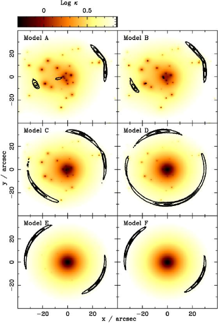
Figure 2: The surface mass density and lensed arcs of the model lensing clusters. The panels are for models A-F in Table 1. The colour-scale shows the surface mass density of the cluster. The lines show the contours that contain 10, 68 and 90 per cent of the total source flux. The value of $\Gamma$ decreases from left to right and top to bottom. Note that for larger values of $\Gamma$, that is, for larger amounts of substructure, the arcs are broken and distorted in several places due to the presence of the individual galaxies.

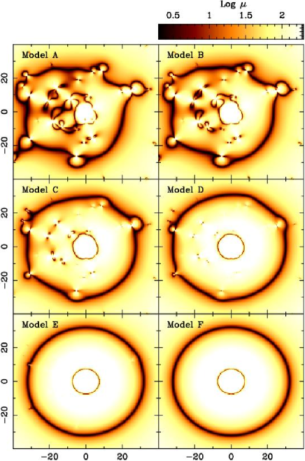
Figure 3: The image magnification maps of the model lensing clusters. The panels are for models A-F in Table 1 and show the magnification of point sources as a function of image position.

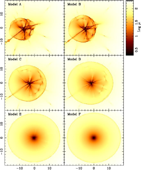
Figure 4: The magnification map on the source plane for the model lensing clusters. As for Fig. 2, the panels are for models A-F in Table 1. The scale is logarithmic for all plots.

Figs. 2 and 3 show the surface mass density of the clusters we used as mass model template and the resulting magnification patterns on the image plane. The magnification maps show the magnification $\mu$ of a point source as a function of position. The corresponding magnification maps on the source plane are shown in Fig. 4. The high magnification regions on the image and source planes are the ‘critical’ and ‘caustic’ lines respectively. Note that the structure of the critical lines, for $\Gamma>0.5$ are very similar to the ones obtained from lens mass reconstructions of observed clusters (Kneib et al., 1996; Broadhurst et al., 2005).

These figures demonstrate that increasing the mass in the individual galaxies, and thereby increasing the amount of substructure, creates more strongly distorted critical lines. Any long arcs of highly magnified sources that are produced along the strongly curved sections of the critical lines will appear broken and distorted. Therefore, the probability of observing broken and distorted arcs increases with increasing fraction of the total cluster mass that resides in individual galaxies. For most of the remainder of this paper we will use a model with a very strong amount of substructure (model A). This model probably represents an extreme case. Since we expect the accuracy with which the source can be reconstructed to decrease with increasing amount of substructure, this will be a ‘worst-case’ scenario for any reconstruction method.

2.4 Generating a lensed data cube using ray-tracing

In order to obtain simulated images of the source at different wavelengths, we use the ray-tracing code gLens, previously used for several lensing studies (Möller & Blain, 1998, 2001; Möller et al., 2003). All pixels of a given image are mapped from the image plane onto the source plane. The flux of the $i$th pixel in the image plane, $f_{i}=F^{\mathrm{I}}(\theta_{i})$, is set using the flux on the source plane $F^{\mathrm{S}}$ from $F^{\mathrm{I}}(\theta_{i})=F^{\mathrm{S}}\left(\theta_{i}-\alpha_{i}\frac{D_{\mathrm{LS}}}{D_{\mathrm{OS}}}\right)$. This method works well and is very robust, but is not the most efficient way to calculate images of extended sources. For example, many pixels are mapped to the empty regions in the source plane. Ray-tracing of these ‘empty’ rays could be avoided using some sort of adaptive algorithm (Möller & Blain, 2001). However, for the purpose here the non-adaptive approach is sufficient. The ray-tracing technique is extremely accurate. Numerical artefacts appear only when there is a strong mismatch between the source and image plane resolutions or dimensions. In this paper, the image plane has a size of $120\times 120$ arcsec and a resolution of $N=1200\times 1200$ pixels. This image plane is mapped onto a source plane of $800\times 800$ pixel resolution, covering an area of $40\times 40$ ″. With these settings numerical errors are negligible.

3 Properties of lensed arcs

Several strongly lensed arcs have been discovered to date (e.g. Fort et al., 1988; Kneib et al., 1995; Luppino et al., 1999; Gladders et al., 2003; Broadhurst et al., 2005). The arcs in Abell 2218 and Abell 370 are perhaps the most notable of these, being up to 20 arcsec long and 2-3 arcsec wide. Smaller arcs have been discovered in some other clusters, like CL 1358+62. In these clusters, the arcs are usually less extended in both directions with lengths of a few arcseconds and widths $\sim 1$ arcsecond. It is important to make a distinction here between arcs that are produced by galaxy lenses and arcs that are lensed by massive clusters. The lengths and widths are quite different. An example of an arc produced in strong galaxy-galaxy lensing is the most prominent arc in the Ultra Deep Field (Blakeslee et al., 2004, UDF). The lensing galaxy is a field elliptical, much less massive than the central cD galaxies in massive clusters. The arc is only $\sim 0.3$ arcsec wide and about $\sim 1$ arcsec long.

We show the resulting images of our simulated lensed arcs as contours in Fig. 2. The simulated arcs for models A and B are very similar to those actually observed for several cluster lenses and show the main features clearly: a broken structure caused by the individual galaxies in the lens. The arc lengths and widths of $\sim 10$ arcsec and $\sim 2$ arcsec, respectively, are very comparable to observed widths and lengths. The smoother potentials of models C-F lead to continuous, smoother arcs. The appearance of the lensed arcs is very similar to observed arc systems for models A and B and we therefore use only these two models for the remainder of this paper.

4 The velocity fields of simulated arcs

4.1 Smooth sources

Using the ray-tracing procedure described in § 2.4 we calculated the individual channel maps of the lensed source, modeled as described in § 2.3. The velocity fields of the strongly lensed arcs are determined by fitting gaussians to the line profiles. In this section, we do not include observational effects, like seeing, coarse instrument resolution or noise. These will be discussed in § 6.

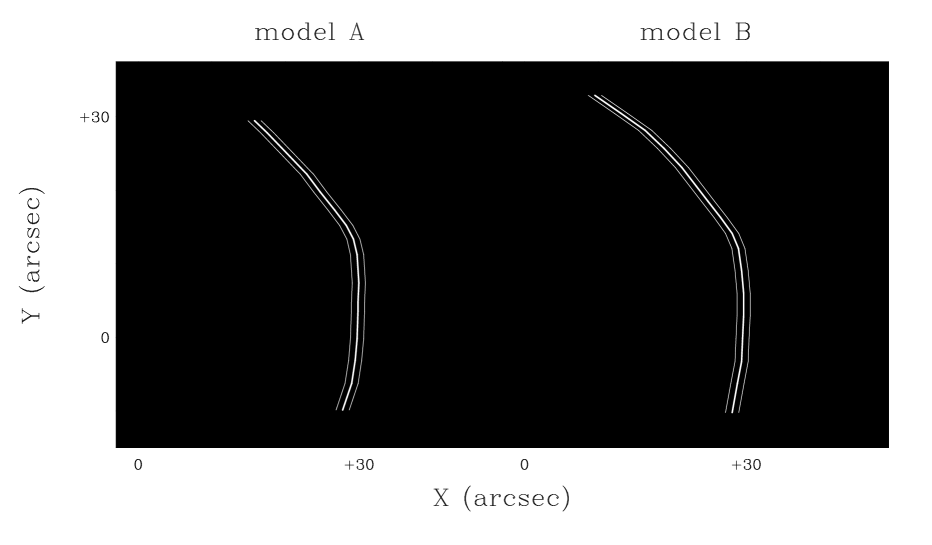
Figure 5: Velocity fields for an extended source lensed by a galaxy cluster. The parameters for the lens and source are as in the previous figure for model A and B. The white lines indicate slices along which the position-velocity diagrams are determined (shown in Fig. 6). The colour scale is the same as for the inset in Fig. 1

We show the lensed velocity fields of the main arcs for models A and B in Fig. 5. The resulting velocity structure is very complex. Gravitational lensing into multiple images produces a very distorted and asymmetric velocity structure along the arc. When velocity information of a lensed arc is available, the source can be essentially broken down into several smaller components which cover different parts of the source plane and are therefore all magnified and distorted in a different way. This effect of differential magnification was already discussed in § 2.1 and, in a different context, by Blain (1999). The small difference between models A and B in terms of the mass distribution within the cluster (in model A, the galaxy that is closest to the arc has a velocity dispersion of $248\,\mathrm{km\,sec^{-1}}$, in model B it is $223\,\mathrm{km\,sec^{-1}}$) translates into a noticeable and measurable difference in the velocity fields: in model B, the regions with approaching velocities are more strongly magnified relative to the receding side.

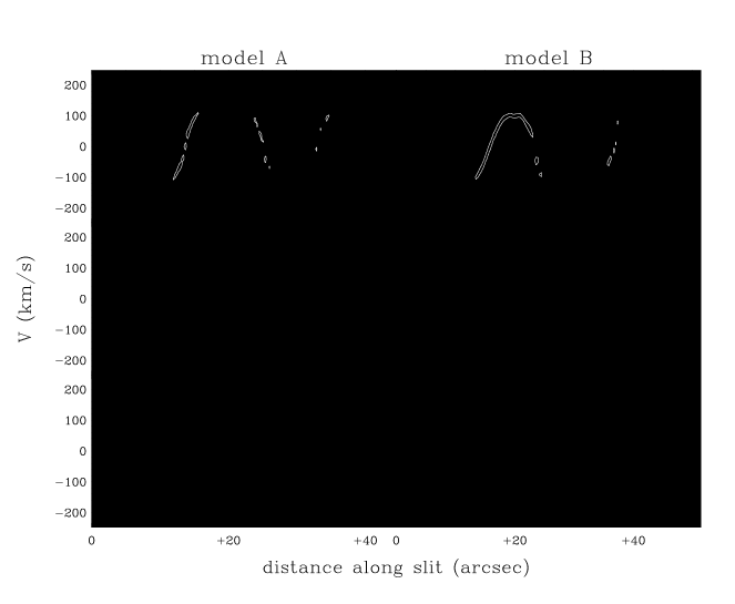
Figure 6: Position-velocity diagram along the main lensed arcs. Only the velocity profiles for models A and B are shown. Panels (a) and (b) show the position-velocity diagram along a line following the brightest pixels on the arc (the thick white line in Fig. 5). In panels (c) and (d) this line is offset by +3 pixels ($\approx$ 1 arcsec) in x, in panels (e) and (f) it is offset by -3 pixels in x. The contours correspond to the maximum intensities at 1, 3 and 5 radial scalelengths in the input model (cf. Fig. 1). For all offsets the position-velocity diagram is heavily distorted with respect to the unlensed case.

The left and right panels in Fig. 6 show the position velocity diagrams for model A and model B, respectively. The positions of the curved slits used to generate the position velocity diagrams are indicated in Fig. 5 by the white lines. They have a width of 1 pixel or $0.3\,$ arcsec. A broader slit would increase the velocity range at each position element and the curves would become broader. The two lower sets of panels show the results if the original slit is displaced by $\pm 3$ pixels or $\pm 1$ arcsec. This changes the regions along the velocity field of the lensed arc that are probed, leading to changes in the shape of the curve. In particular, remarkable features like strong asymmetry in the position-velocity diagram may result; as seen in panels (c) and (d). Note that none of the lensed position-velocity slices resemble those of unlensed galaxies. It is also noteworthy that the lensed position-velocity slices shown here look very similar to those observed by Pelló et al. (1991, Fig.4).

There is another simple and drastic effect that gravitational lensing has on the velocity structure of sources, which can be demonstrated easily by looking at the total flux emitted as a function of channel. Fig. LABEL:fig.cluster.flux shows the flux ratio $F(\nu)/F_{\mathrm{tot}}$ in the main arc (top) and the corresponding ratio $F(\nu)/F_{\mathrm{tot}}$ for the counter arc (bottom). In both cases, $F({\nu})$ and $F_{\mathrm{tot}}$ are given by eqs. 9 and 7, respectively. Comparison with the unlensed case, as shown by the dotted line in Fig. LABEL:fig.cluster.flux, shows the effect of differential magnification very clearly. For most models, the parts of the source with velocities around $-100\,\mathrm{km}\,\mathrm{s}^{-1}$ are magnified more strongly than the rest of the galaxy. For a symmetric galaxy such a profile is a strong indication of differential magnification. For a single arc, this effect may also be reproduced without differential magnification when there is strong asymmetrical substructure in the source (Richter & Sancisi, 1994). Differential magnification can either enhance or partially cancel intrinsic asymmetries in the source. However, since the differential magnification is strongly influenced by the small scale – and hence local – structure in the lensing potential, lensing will in general produce different asymmetries in different arcs of the same source. In the given case, a comparison between the fluxes for the main arc, in the top panel of Fig. LABEL:fig.cluster.flux, and the counter arc, in the bottom panel, shows that the asymmetries are induced by lensing. In this way, asymmetries induced by lensing can be distinguished from intrinsic asymmetries, which affect all arcs of a given source.

4.2 Source substructure

Throughout we have assumed a smooth light distribution for our source galaxy. At high redshifts the merger rate is expected to be much higher than in the local universe (Patton et al., 2002), and consequently galaxies may show far more substructure and kinematic signatures of merger events (Naab & Burkert, 2003). Currently, there is still some uncertainty as to how much of the difference in the morphology and observed light distribution of high redshift galaxies is due to intrinsic differences and how much is due to the fact that the optical at a redshift of $z\sim 1$ corresponds to restframe UV. Due to regions of star formation, local late-type galaxies are found to show much more substructure when observed in the UV. How would our results change if the source light distribution is intrinsically less smooth ? As long as the underlying kinematics does not change, we find that the clumpiness of the source has little effect on the results discussed in the previous sections. This is illustrated in Fig. LABEL:fig.clumpy, where we show the clumpy source and the position velocity diagram along the lensed arc, which has the same shape and position as for the smooth source model. Apart from many discontinuities in the diagram the shape is the same as in Fig. 6. However, we still assume dynamically stable rotation everywhere within the source. In particular our model assumes that there are no major in- or outflows related to the source. If these are present, as may be expected for a fraction of sources at high redshifts, these will show up as clear signatures in the reconstructed velocity profiles of the lensed arcs. We discuss in more detail how well substructured sources can be reconstructed in § 5.5.

5 Reconstructing the source kinematics and the lens mass distribution

5.1 Reconstruction algorithm

In the previous sections we discussed the velocity structure of lensed arcs of extended sources. Using a simple model for the kinematic structure of the source, we have shown that the observed velocity structure in the arc is complex and depends on the mass distribution in the strong lensing cluster – especially the mass in the galaxies close to the arc.

A remaining question is how well the original velocity structure of the source can be reconstructed from the available channel information of the lensed arc. Clusters of galaxies have been modeled from strong lensing in the past (e.g. Kneib et al., 1998), deriving the cluster potential from the positions and shapes of the arcs. This approach works very well when the overall cluster potential is to be determined. When the source itself is to be reconstructed, it is often necessary to perform more elaborate fits including pixel information (Tyson et al., 1998).

Using our simulated images for cluster model A, we attempt to reconstruct the cluster and source model parameters from the image data alone. We assume that galaxy redshifts and positions in the cluster are known, but not their masses. A number of 14 galaxies are included in the cluster model, in addition to a halo of unknown position and mass. The free source parameters are position, exponential scale length, total flux, position angle and axis ratio. In total we therefore have $14+3+6=23$ free parameters. We use a total of $N_{\mathrm{pix}}=500$ pixels selected randomly from the region around the arc on the image as constraints. Each pixel is mapped onto the source plane and the flux at the source plane position is compared with the flux of the source model. The positions of the pixels themselves also provide a constraint: bright pixels should be clustered more than faint pixels. We include this constraint by first calculating the flux weighed centre of the mapped source pixels,

$$\mathbf{x_{0}}=\frac{\sum_{i=1}^{N_{\mathrm{pix}}}f_{i}\mathbf{x_{i}}}{\sum_{i=1}^{N_{\mathrm{pix}}}f_{i}}$$ (15)

and then calculating the distance of each pixel with respect to this flux weighed centre. The total ‘goodness’, $\xi$ is then calculated as:

$$\xi^{2}=\sum_{i=1}^{N_{\mathrm{pix}}}|\mathbf{x_{i}}-\mathbf{x_{0}}|^{2}f_{i}^{2}+(f_{i}-m_{i})^{2}.$$ (16)

In this equation, $m_{i}$ is the model flux at pixel $i$. Note that we include a dependence on the pixel positions $f_{i}$ in the first term, since in our source model brighter pixels are required to be more compact than fainter pixels. Also, note that this definition is only useful for determining the best fit models – a meaningful $\chi^{2}$ value can only be defined on the image plane. This is done below in § 5.2.

In order to obtain an acceptable fit, and also to include possible degeneracies, we perform the fitting using a modified simulated annealing technique, with slow cooling. A population of 400 model clusters, initially randomly sampling the parameter space in a uniform manner, is slowly adjusted in 4000 steps. At each step, a new point in parameter space is chosen, sampling the logarithmic parameter space using a Monte Carlo Markov Chain (MCMC) method. After each step, the new set of model parameters replaces the old one with a probability given by

$$p_{\mathrm{replace}}=\mathrm{min}\left(e^{(\chi_{\mathrm{old}}-\chi_{\mathrm{new}})/T},1\right),$$ (17)

where $T$ is the current ‘temperature’ of the system, which is cooled from $T_{\mathrm{start}}=10$ to $T_{\mathrm{end}}=0.001$ in the 4000 steps logarithmically. From the final sample of 400 models, we select the 9 best-fitting models.

5.2 The reconstructed sources

The contours in Fig. LABEL:fig.velbest show isophotes of the resulting source reconstructions for the 9 best-fitting lens models. These source reconstructions are calculated by ray-tracing the original, ‘observed’ image to the source plane through the corresponding reconstructed model of the lens. All sources are compact and in rough agreement with the input position angle and inclination. Most importantly all the best-fitting models give source models with an integrated light profile that is consistent with an exponential disc profile.

We define a goodness of fit in the image plane as

$$\chi^{2}=\sum_{i=1}^{N}\left(\frac{f_{i}-m_{i}}{\sigma_{i}}\right)^{2}w_{i},$$ (18)

where

$$w_{i}=\frac{f_{i}+m_{i}}{\sum_{j=1}^{N}f_{j}+m_{j}},$$ (19)

and $\sigma_{i}=5\times 10^{-5}$ is our assumed surface brightness error in units of the total flux of the source. With this definition, $\chi^{2}\sim 1-3$ in all of these cases. The velocity fields of the best-fitting reconstructed sources are displayed with the colour scales in Fig. LABEL:fig.velbest. Most of the reconstructed velocity fields show the same global shape as the input model, but in several cases distortions are present, especially in the outer parts. These distortions are inconsistent with dynamically stable rotation and can be used to distinguish between the different reconstructions.

To investigate which reconstructed velocity fields are consistent with regularly rotating gas discs, we tried to fit each of them with tilted ring models. In these fits, gas is assumed to move on circular orbits around the centre of the galaxy in a series of concentric rings. The position angle and inclination of the galaxy, as well as the rotation velocity of each ring is fitted to obtain the best match with our ‘observed’ reconstructed velocity field. The differences between the lens reconstructions of the source kinematics and our best tilted ring fits are shown in Fig. LABEL:fig.residual for all reconstructions. For the majority of cases, the differences in the central regions of the source are small, but larger in the outer, high-velocity regions of the source. However, several reconstructions (e.g. 2, 5 and 8) show significant distortions in the inner regions. Such distortions are not observed in real galaxies and must therefore be due to an imperfect lens model.

5.3 Comparison of isophotal and kinematic fits

Even though the source light profile is acceptable for all reconstructions, close inspection of the velocity fields shows that some of the lens models are insufficiently accurate to allow reconstruction of the source kinematics. To investigate this further, we also performed an isophotal analysis of the reconstructed images and compared the morphological orientation of the reconstructed sources with the kinematical orientation as derived from the tilted ring fits.

Reconstruction	$\phi_{\mathrm{kin}}$	$\theta_{\mathrm{kin}}$	$\phi_{\mathrm{iso}}$	$\theta_{\mathrm{iso}}$
1	6$\pm$2	39$\pm$5	14$\pm$2	51$\pm$1
2	-1$\pm$1	33$\pm$6	-16$\pm$3	40$\pm$2
3	1$\pm$1	37$\pm$4	-1$\pm$1	39$\pm$2
4	1$\pm$1	49$\pm$2	1$\pm$1	51$\pm$1
5	13$\pm$2	25$\pm$10	-59$\pm$3	35$\pm$3
6	-2$\pm$1	34$\pm$4	-14$\pm$1	39$\pm$2
7	-2$\pm$1	44$\pm$2	0$\pm$2	46$\pm$1
8	13$\pm$2	42$\pm$5	17$\pm$2	55$\pm$1
9	-2$\pm$1	52$\pm$1	3$\pm$ 1	55$\pm$1
C1	0$\pm$1	40$\pm$4	11$\pm$7	39$\pm$4
C2	-3$\pm$2	33$\pm$5	2$\pm$12	38$\pm$4
C3	-4$\pm$1	51$\pm$2	-21$\pm$2	49$\pm$3

Table 2: Parameters of the source reconstructions for the 9 best-fitting lens models. The values for the position angle from isophotal and tilted ring fits, $\phi_{\mathrm{iso}}$ and $\phi_{\mathrm{kin}}$ are listed together with the corresponding inclination angles, $\theta_{\mathrm{iso}}$ and $\theta_{\mathrm{kin}}$. Also shown are the results for the substructured models C1, C2 and C3, discussed in § 5.5.

The derived values for the position angle and inclination from both analyses are listed in Table 2. Comparing the position angles of the isophotal analysis to those obtained from the tilted ring fits shows a large discrepancy of 10 or more degrees for several reconstructions (2, 5, 6). The inclination angles from the isophotal and tilted ring fits agree to within 10 degrees in all cases. The inclination angles from isophotal fits are within 10 degrees of the input value of 50 degrees with the only exception of reconstruction 2 which has a best fit inclination angle of 35 degrees. Only for models 3, 4, 7 and 9 is $|\theta_{\mathrm{iso}}-\theta_{\mathrm{kin}}|\mathrel{\hbox{\hbox to0.0pt{\hbox{\lower 4.0pt\hbox{$\sim$}}\hss}\hbox{$<$}}}5$ degrees. Inspecting the residuals between the velocity fields as fitted with the tilted ring models and the reconstructed velocity fields, shown in Fig. LABEL:fig.residual, also helps to discriminate different models. The strongest residuals in the central parts – that is inside the contours in each panel of Fig. LABEL:fig.residual – are associated with the reconstructions for models 1, 2, 5 and 8.

On the basis of the information from Table 2 and Fig. LABEL:fig.residual, one would draw the conclusion that reconstructions 3, 4, 7 and 9 are the most accurate. From these, one would constrain the position angle and inclination angle of the source to be $\frac{1}{2}(\phi_{\mathrm{kin}}+\phi_{\mathrm{iso}})=0.2\pm 0.5$ degrees and $\frac{1}{2}(\theta_{\mathrm{kin}}+\theta_{\mathrm{iso}})=47\pm 3$ degrees – consistent with the input values.

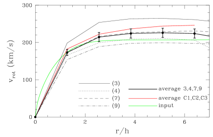
Figure 7: Rotation curves from tilted ring fits. The thin black lines give the rotation curves derived from the velocity fields from reconstructions 3, 4, 7 and 9 from Table 2. The bold line with data points shows the average of the 4 individual curves; the errorbars are estimated as 1/2 of the rms scatter of the points from the individual curves. The solid, thin green line shows the input rotation curve from eq. 11. The red line shows the result for the average of the three best fits to the substructured source (cf. § 4.2).

In Fig. 7, we show the rotation curves derived from the tilted ring fits for these reconstructions, together with the average of all 4 and the input rotation curve from eq. 11. Within the expected observational uncertainties these reconstructed velocity fields allow an accurate recovery of the input rotation curve.

5.4 Effect of cluster mass profile and ellipticity

Thus far we have assumed a cored pseudo-isothermal model for the cluster halo mass distribution in our model. The total mass profile in our model cluster follows an NFW form only due to added substructure in the form of galaxies. A pseudo-isothermal mass profile has been shown to provide good fits to lensing cluster halos in previous studies (Sand et al, 2005; Kneib et al., 1996). Numerical simulations, however, predict that cluster halo mass profiles follow a NFW form more closely. In addition, we have assumed a spherical mass distribution for the cluster, whereas most real and simulated clusters have elliptical mass profiles. There is a degeneracy here between the ellipticity of the halo mass profile and the presence of massive substructure, as both induce an asymmetric lensing potential. The effect of triaxiality on lensing statistics has also been found to be degenerate with core size by Oguri et al. (2005). We have tested how strongly ellipticity in the lens model affects the properties of the arcs and the reconstructed source.

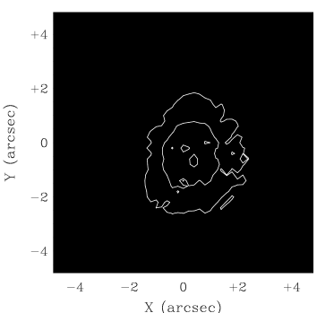
Figure 8: The reconstructed source kinematics of the best-fit elliptical NFW cluster lens model. The original simulated data (shown in Fig. 2) is fitted with an elliptical NFW halo model with three cluster galaxies. The figure shows the reconstructed integrated light profile (contours) and velocity field (colour) of the source. The best-fit NFW lens model has an ellipticity of $\epsilon=\sqrt{1-b^{2}/a^{2}}=0.15$, where $a$ and $b$ are the major and minor axes, respectively. Its virial mass $M_{\mathrm{vir}}=1.925\times 10^{14}M_{\odot}$ and its concentration parameter is $c=5.6$ (see Navarro et al. (1997) for a definition of these parameters).

Fig.  8 shows the reconstructed source properties for the best fitting model of an elliptical NFW cluster halo with three additional cluster galaxies. A relatively good fit to the source light profile is retained. However, the model fails in reproducing the small scale details of the velocity structure of the source; the velocity field in the central region is bend into an ‘S’-shaped structure. In principle, high quality kinematic data could break the degeneracy between halo ellipticity and massive substructure. In practice, however, it is doubtful whether current instruments could provide data that would be accurate enough to detect these small scale differences.

5.5 Fits to substructured sources

Above we discussed how the appearance of the velocity field of arcs would change if sources are substructured instead of smooth. Since such substructures would produce additional uncertainties in any source reconstructions, we also perform fits to a substructured source model using our method. The velocity fields and residuals to tilted ring fits for the three best fitting reconstructions C1-C3 are shown in the bottom row of Figs. LABEL:fig.velbest & LABEL:fig.residual, respectively. Models C1 and C2 show a low residual to the tilted ring fit, whereas model C3 shows some velocity distortions in the central region and appears slightly more compact overall. Averaging the resulting best-fit rotation curves for these three reconstruction gives an averaged inclination angle of $42\pm 4$deg and an average position angle of $4\pm 1$ deg. These values are within 2$\sigma$ of the input. The averaged rotation curve is shown as the red line in Fig. 7.

5.6 The lens mass reconstructions

We investigated what differences in the lens mass reconstructions lead to the observed differences in source reconstructions. Inspecting the reconstructed mass maps and calculating the total mass inside the Einstein radius for all the reconstructions, we found that there are only very small differences between the different reconstructions; the total mass within an Einstein radius is always within 1-3% of the input value. However, there are larger differences in how the mass is distributed within the Einstein ring; the reconstructions differ in their amount and direction of asymmetry in the central regions. In addition, the surface mass density in regions away from the main arc vary by $\sim 30-50\%$ between the reconstructions. This large variation is to be expected as the main constraints on the lensing mass distribution comes from the main arc itself and is, strictly, only a local constraint on the mass distribution. It is only due to the parameterised form of the input model that the arc constrains other regions in the cluster at all. The differences in the reconstructions of the velocity fields mainly come from the change in the distribution of mass in the central part of the cluster and from small changes in the mass of the galaxies very close to the main arc.

6 Observational possibilities

In the previous sections, we have shown how gravitational lensing affects the velocity fields of high-redshift background galaxies, and how the additional information contained in the observed velocity fields can be used to constrain models of the lensing cluster and source galaxy. In this section, we will discuss the possibilities of observing the velocity fields of strongly lensed galaxies.

It is clear from the previous sections that one needs to measure velocities over the full 2D extent of an arc, in order to use the kinematic information to constrain the lens model and to determine the rotation curve of the source galaxy. Simple long slit spectra along lensed arcs lack information about the orientation of the source galaxy, making it impossible to interpret the kinematic properties of the arc unambiguously. Additionally, small slit offsets and finite slit widths have a strong effect on the observed profiles, as can be appreciated from the difference between for example panels (a), (c) and (e) in Fig. 6.

To observe the velocity fields of giant arcs, integral field spectroscopy at high spatial resolution and high sensitivity is required. Our simulated lensed velocity maps in Fig. 5 have a width of about $5$ arcseconds, but one should bear in mind that in producing these figures, we have not applied any flux-cut. In reality, velocities can only be measured in the brighter regions of the arcs, with a typical width of $1$ arcsecond. Spatial resolution of at least 0.2–0.3 arcseconds is required to resolve these regions. The demands on spectral resolution are less stringent. Typical spiral galaxies have rotation velocities in the range 100–300 km/s, so a velocity resolution of order 50–100 km/s is sufficient to measure radial velocities of the gas to a fraction of the expected rotation velocities.

To carry out the required observations, a number of options are available. Currently, the best opportunity is offered at optical or near-infrared wavelengths, where, depending on the source redshift, several strong emission lines of ionised gas (e.g. H$\alpha$, Oii, Oiii, etc.) are available. Sub-arcsecond seeing is now routinely achieved with adaptive optics systems at a number of ground-based telescopes, and the number of integral field spectrographs that make use of the high resolution offered by these systems is rapidly increasing (e.g. GMOS on Gemini and Sinfoni on the VLT). The biggest obstacle currently seems to be that, in order for adaptive optics systems to deliver the sub-arcsecond images, a bright ($m_{V}\mathrel{\hbox{\hbox to0.0pt{\hbox{\lower 4.0pt\hbox{$\sim$}}\hss}\hbox{$<$}}}14$) guidestar in the immediate neighbourhood of the object is required. Since most lensed arcs do not lie close enough to such a bright star, one has to await the development of artificial laser guide-star systems to observe the most interesting arcs. However, technology seems to be improving rapidly, and several observatories expect a working system within a few years from now.

All giants arcs observed hitherto are intrinsically faint, so large telescopes are required to obtain useful spectra. Long-slit spectra of a straight arc at $z=0.91$ have been obtained by Pelló et al. (1991), using a $2$ arcsec wide slit at the 4.2m WHT. In 15 hours of integration time, they obtained a high signal-to-noise ratio spectrum which enabled them to extract velocities along the full length ($>10$ arcsec) of the arc. Several other groups have recently measured spatially resolved velocities in unlensed galaxies out to redshifts of $z\sim 2$, using 8–10m class telescopes like Keck or VLT and slitwidths of 0.5–1.0 arcsec (Vogt et al., 1996; Vogt et al., 1997; Böhm et al., 2004; Erb et al., 2004). These results imply that at 8–10m class telescope like the VLT, Keck or Gemini, sub-arcsecond resolution observations should be feasible in 1–2 nights of integration time.

Other options lie further in the future. ALMA is currently being constructed, and will offer the required resolution and sensitivity to observe the kinematics of molecular gas at the redshifts of the arcs we study here. Even further ahead, giant radiotelescopes like SKA will be able to observe the Hi emission line of neutral hydrogen. This would offer the fascinating possibility of measuring the kinematics of lensed galaxies well outside their stellar discs, probing into the dark matter dominated regions of these young galaxies. Finally, several studies are currently underway to design the next generation optical telescopes, with diameters of 25 meter and larger. With the light gathering powers of such extremely large telescopes, it will be feasible to detect emission lines out to large galactocentric distances in lensed arcs within very short exposure times, thus enabling systematic studies of the kinematics of these high-redshift galaxies.

7 Discussion and Conclusions

Determining the properties of high redshift galaxies remains one of the main goals of current research. In this paper, we presented a first theoretical investigation on how the effect of gravitational lensing can be exploited to determine the kinematic properties of high redshift galaxies.

Using a parametric cluster model we simulated the velocity structure of strongly lensed background galaxies. The combination of ray-tracing techniques with parametric cluster and source models proved to be a very efficient and accurate method for this study.

In general, we found that the two dimensional kinematic profile along strongly lensed arcs is very complex. Differential magnification leads to very distorted position-velocity diagrams and strong asymmetries in the velocity fields. Here, it is important to note that the individual cluster galaxies close to the arc contribute strongly to this effect, as we demonstrated in sections 4 and 5. Using a relatively simple-minded technique, we showed that reconstructions of the 2D kinematic source properties of lensed arcs are in principle possible. Since the velocity structure is sensitive to small variations in the lensing potential, kinematic information along the arc provides additional tight constraints on the mass distribution in the proximity of lensed arcs. Observationally, the use of an integral field spectrograph at an 8–10m class telescope with sub-arcsecond seeing will allow accurate source reconstructions and measurements of the rotation curve of strongly lensed arcs. We predict that the inclination and position angles of sources that are dynamically stable rotators can be determined to an accuracy of $\sim 10\%$. Rotation curves can thereby be determined with accuracies of better than $15\%$ out to 2–3 disc scale lengths for galaxies at redshifts above $z\sim 1.5$ in this way.

Our general approach was motivated by our aim to provide a general discussion of the kinematic properties of lensed arcs and point out the uses and possibilities of kinematic data of such systems. The parametric cluster model we used was simple, but it reproduced the observed appearance of strongly lensed arcs well, when the galaxy mass-fraction inside the cluster Einstein radius was high. We note here that it should be possible to constrain the mass fraction of galaxies in clusters by making statistical predictions about the shape of arcs, for example from N-body simulations, and comparing them with the observed structure of arcs. A thorough study of this would have to take into account the effect of cluster merging and the mass function of cluster sub-haloes. Our predictions for the general appearance of velocity fields of arcs are independent of the specific form of the cluster potential, as long as the observed properties of arcs are reproduced. This is because any other description of the cluster potential must also reproduce the observed properties of lensed arcs. In particular, the local differential magnification that produces the distortions in the velocity fields arises from small scale mass structures close to the arcs, which are also responsible for the broken structure of observed arcs.

Our method here has made use of a smooth source model. Even though we demonstrated that structure in the source does not change our results and does not affect the appearance of arcs and their velocity fields significantly, this is strictly only true as long as the source itself has stable rotation. For high redshift sources that will probably not always be true, since mergers, outflows etc. are much more common at higher redshifts. However, as we pointed out, one of the advantages of the multiple arc systems formed by lensing is that intrinsic properties of the source can be disentangled from lensing induced distortions. Lensing distortions will be different for each arc, since the local cluster mass structure is important, whereas intrinsic source properties are the same for all arcs from a single source. In fact, this can be exploited to the extent that the source and lens can be reconstructed from arcs without (almost) any assumptions about the source itself. Warren & Dye (2003) describe a method that exploits this and can reconstruct the lens and source in the presence of noise and finite seeing. Such a non-parametric method was previously described by Wallington et al. (1996, 1994) and extended by Koopmans (2005). It can be applied equally well to reconstruct the kinematic source properties, independent of any assumptions about the source – except that the source be of a physically plausible size.

In this paper we concentrated entirely on arcs produced by clusters. This was motivated by the fact that cluster arcs are larger and easier to distinguish from light emission originating from the lens plane. Galaxy lenses produce considerably smaller arcs that are superimposed on the lens galaxy itself. However, with IFU’s of high spatial resolution it may be possible to determine the kinematic profile of arcs lensed by galaxies as well. Since the relative scale of source to lens is about unity for galaxy lenses, in contrast to cluster lenses where it is much smaller, the appearance of the arcs produced by galaxy lenses is much smoother than for cluster lenses. This can be explained by noticing that a version of, for example, the top left panel in Fig. 4 that is scaled down by a factor of 10 or more would be covered almost completely by the source. This means that small scale structure in the lensing potential would have almost no effect on the overall appearance of the lensed arcs. However, if kinematic data is available, the situation changes. Differential magnification becomes important for each individual channel since a given velocity channel only probes a very small region on the source plane. In other words, kinematic data of arcs behind galaxy lenses can provide strong constraints on the amount of mass in small scale structures of galaxy haloes, and may be used as a direct probe of the mass function at the low-mass end – possibly down to $\sim 10^{7}M_{\odot}$. We will address this in more detail in a future publication.

In summary, it is clear that obtaining two dimensional kinematic profiles of strongly lensed arcs will provide very useful information of both source and lens. Using IFU’s in the very near future to study these systems will provide a unique way to determine the rotation curve of strongly magnified galaxies at redshifts $z\sim 1.5$ or higher and measure their mass-to-light ratio out to several disc scale-lengths.

References

- Böhm et al. (2004) Böhm A., Ziegler B. L., Saglia R. P., Bender R., Fricke K. J., Gabasch A., Heidt J., Mehlert D., Noll S., et al ., 2004, A&A, 420, 97
- Bartelmann et al. (1998) Bartelmann M., Huss A., Colberg J. M., Jenkins A., Pearce F. R., 1998, A&A, 330, 1
- Bartelmann & Weiss (1994) Bartelmann M., Weiss A., 1994, A&A, 287, 1
- Blain (1999) Blain A. W., 1999, MNRAS, 304, 669
- Blain et al. (1999) Blain A. W., Smail I., Ivison R. J., Kneib J.-P., 1999, MNRAS, 302, 632
- Blakeslee et al. (2004) Blakeslee J. P., Zekser K. C., Benítez N., Franx M., White R. L., Ford H. C., Bouwens R. J., Infante L., Cross N. J., Hertling G., Holden B. P., Illingworth G. D., Motta V., Menanteau F., Meurer G. R., Postman M., Rosati P., Zheng W., 2004, ApJL, 602, L9
- Blandford & Narayan (1992) Blandford R. D., Narayan R., 1992, ARA&A , 30, 311
- Broadhurst et al. (2005) Broadhurst T., Benítez N., Coe D., Sharon K., Zekser K., White R., Ford H., Bouwens R., Blakeslee J., Clampin 2005, ApJ, 621, 53
- Bunker et al. (2000) Bunker A. J., Moustakas L. A., Davis M., 2000, ApJ, 531, 95
- Bunker et al. (1999) Bunker A. J., Warren S. J., Clements D. L., Williger G. M., Hewett P. C., 1999, MNRAS, 309, 875
- Ciardi & Ferrara (2005) Ciardi B., Ferrara A., 2005, Space Science Reveiews, 116, 625
- Cooray (1999) Cooray A. R., 1999, A&A, 341, 653
- Dalal et al. (2004) Dalal N., Hennawi J., Bode P., 2004, ArXiv Astrophysics e-prints
- de Blok & Bosma (2002) de Blok W. J. G., Bosma A., 2002, A&A, 385, 816
- de Blok et al. (2001) de Blok W. J. G., McGaugh S. S., Bosma A., Rubin V. C., 2001, ApJL, 552, L23
- Donato et al. (2004) Donato F., Gentile G., Salucci P., 2004, MNRAS, 353, L17
- Ellis et al. (2001) Ellis R., Santos M. R., Kneib J.-P., Kuijken K., 2001, ApJL, 560, L119
- Erb et al. (2004) Erb D. K., Steidel C. C., Shapley A. E., Pettini M., Adelberger K. L., 2004, ApJ, 612, 122
- Flores et al. (2000) Flores, R. A., Maller, A. H., & Primack, J. R. 2000, ApJ, 535, 555
- Fort et al. (1988) Fort B., Prieur J. L., Mathez G., Mellier Y., Soucail G., 1988, A&A, 200, L17
- Garrido et al. (2002) Garrido O., Marcelin M., Amram P., Boulesteix J., 2002, A&A, 387, 821
- Gladders et al. (2003) Gladders M. D., Hoekstra H., Yee H. K. C., Hall P. B., Barrientos L. F., 2003, ApJ, 593, 48
- Haiman & Holder (2003) Haiman Z., Holder G. P., 2003, ApJ, 595, 1
- Hamana & Futamase (1997) Hamana T., Futamase T., 1997, MNRAS, 286, L7
- Hudson et al. (1998) Hudson M. J., Gwyn S. D. J., Dahle H., Kaiser N., 1998, ApJ, 503, 531
- Hughes et al. (1998) Hughes D. H., Serjeant S., Dunlop J., Rowan-Robinson M., Blain A., Mann R. G., Ivison R., Peacock J., Efstathiou A., Gear W., Oliver S., Lawrence A., Longair M., Goldschmidt P., Jenness T., 1998, Nature, 394, 241
- Kanekar & Chengalur (2003) Kanekar N., Chengalur J. N., 2003, A&A, 399, 857
- Kassiola, Kovner & Fort (1992) Kassiola A., Kovner I., Fort B., 1992, ApJ, 400,41
- Kneib et al. (1998) Kneib J. P., Alloin D., Mellier Y., Guilloteau S., Barvainis R., Antonucci R., 1998, A&A, 329, 827
- Kneib et al. (1996) Kneib J.-P., Ellis R. S., Smail I., Couch W. J., Sharples R. M., 1996, ApJ, 471, 643
- Kneib et al. (2003) Kneib J.-P., Hudelot P., Ellis R. S., Treu T., Smith G. P., Marshall P., Czoske O., Smail I., Natarajan P., 2003, ApJ, 598, 804
- Kneib et al. (1995) Kneib J.-P., Mellier Y., Pelló R., Miralda-Escude J., Le Borgne J.-F., Boehringer H., Picat J.-P., 1995, A&A, 303, 27
- Koopmans & Treu (2002) Koopmans L. . V. E., Treu T., 2002, ApJL, 568, L5
- Koopmans (2005) Koopmans L. V. E., 2005, ArXiv Astrophysics e-prints
- Koopmans et al. (1998) Koopmans L. V. E., de Bruyn A. G., Jackson N., 1998, MNRAS, 295, 534
- Koopmans & Treu (2003) Koopmans L. V. E., Treu T., 2003, ApJ, 583, 606
- Luppino et al. (1999) Luppino G. A., Gioia I. M., Hammer F., Le Fèvre O., Annis J. A., 1999, A&A Supp, 136, 117
- Mathewson et al. (1992) Mathewson D. S., Ford V. L., Buchhorn M., 1992, ApJS, 81, 413
- Mehlert et al. (2001) Mehlert D., Seitz S., Saglia R. P., Appenzeller I., Bender R., Fricke K. J., Hoffmann T. L., Hopp U., Kudritzki R.-P., Pauldrach A. W. A., 2001, A&A, 379, 96
- Mellier (1999) Mellier Y., 1999, ARA&A , 37, 127
- Meneghetti et al. (2003) Meneghetti M., Bartelmann M., Moscardini L., 2003, MNRAS, 340, 105
- Meneghetti et al. (2000) Meneghetti M., Bolzonella M., Bartelmann M., Moscardini L., Tormen G., 2000, MNRAS, 314, 338
- Meneghetti et al. (2004) Meneghetti M., Jain B., Bartelmann M., Dolag K., 2004, ArXiv Astrophysics e-prints
- Meneghetti et al. (2001) Meneghetti M., Yoshida N., Bartelmann M., Moscardini L., Springel V., Tormen G., White S. D. M., 2001, MNRAS, 325, 435
- Möller & Blain (1998) Möller O., Blain A. W., 1998, MNRAS, 299, 845
- Möller & Blain (2001) Möller O., Blain A. W., 2001, MNRAS, 327, 339
- Möller et al. (2003) Möller O., Hewett P., Blain A. W., 2003, MNRAS, 345, 1
- Naab & Burkert (2003) Naab T., Burkert A., 2003, ApJ, 597, 893
- Narasimha & Chitre (1993) Narasimha D., Chitre S. M., 1993, A&A, 280, 57
- Navarro et al. (1997) Navarro J. F., Frenk C. S., White S. D. M., 1997, ApJ, 490, 493
- Oguri et al. (2001) Oguri M., Taruya A., Suto Y., 2001, ApJ, 559, 572
- Oguri et al. (2005) Oguri M., Takada M., Umetso K., Broadhurst T., 2005, ArXiv Astrophysics e-prints
- Palunas & Williams (2000) Palunas P., Williams T. B., 2000, AJ, 120, 2884
- Patton et al. (2002) Patton D. R., Pritchet C. J., Carlberg R. G., Marzke R. O., Yee H. K. C., Hall P. B., Lin H., Morris S. L., Sawicki M., Shepherd C. W., Wirth G. D., 2002, ApJ, 565, 208
- Pelló et al. (1999) Pelló R., Kneib J.-P., Le Borgne J. F., Bézecourt J., Ebbels T. M., Tijera I., Bruzual G., Miralles J. M., Smail I., Soucail G., Bridges T. J., 1999, A&A, 346, 359
- Pelló et al. (1991) Pelló R., Sanahuja B., Le Borgne J., Soucail G., Mellier Y., 1991, ApJ, 366, 405
- Persic & Salucci (1995) Persic M., Salucci P., 1995, ApJS, 99, 501
- Persic et al. (1996) Persic M., Salucci P., Stel F., 1996, MNRAS, 281, 27
- Richard et al. (2003) Richard J., Schaerer D., Pelló R., Le Borgne J.-F., Kneib J.-P., 2003, A&A, 412, L57
- Richter & Sancisi (1994) Richter O.-G., Sancisi R., 1994, A&A, 290, L9
- Sand et al (2005) Sand D., Treu T., Ellis R. S., Smith G. P., 2005, ApJ, 627, 32
- Smail & Dickinson (1995) Smail I., Dickinson M., 1995, ApJL, 455, L99
- Swaters (1999) Swaters R. A., 1999, PhD thesis, Rijksuniversiteit Groningen
- Swinbank et al. (2003) Swinbank A. M., Smith J., Bower R. G., Bunker A., Smail I., Ellis R. S., Smith G. P., Kneib J.-P., Sullivan M., Allington-Smith J., 2003, ApJ, 598, 162
- Tully & Fisher (1977) Tully R. B., Fisher J. R., 1977, A&A, 54, 661
- Tyson et al. (1998) Tyson J. A., Kochanski G. P., dell’Antonio I. P., 1998, ApJL, 498, L107+
- Verheijen & Sancisi (2001) Verheijen M. A. W., Sancisi R., 2001, A&A, 370, 765
- Vogt et al. (1997) Vogt N. P., Phillips A. C., Faber S. M., Gallego J., Gronwall C., Guzman R., Illingworth G. D., Koo D. C., Lowenthal J. D., 1997, ApJL, 479, L121
- Vogt et al. (1996) Vogt N. P., Phillips A. C., Faber S. M., Illingworth G. D., Koo D. C., 1996, Bulletin of the American Astronomical Society, 28, 1413
- Wallington et al. (1996) Wallington S., Kochanek C. S., Narayan R., 1996, ApJ, 465, 64
- Wallington et al. (1994) Wallington S., Narayan R., Kochanek C. S., 1994, ApJ, 426, 60
- Wambsganss et al. (2004) Wambsganss J., Bode P., Ostriker J. P., 2004, ApJL, 606, L93
- Wambsganss et al. (1998) Wambsganss J., Cen R., Ostriker J. P., 1998, ApJ, 494, 29
- Warren & Dye (2003) Warren S. J., Dye S., 2003, ApJ, 590, 673
- Williams et al. (1999) Williams L. L. R., Navarro J. F., Bartelmann M., 1999, ApJ, 527, 535
- Wu & Mao (1996) Wu X., Mao S., 1996, ApJ, 463, 404
- Zhao & Qin (2003) Zhao H., Qin B., 2003, ApJ, 582, 2