An empirical calibration of sulphur abundance in ionised gaseous nebulae

We have derived an empirical calibration of the abundance of S/H as a function of the S₂₃ parameter, defined using the bright sulphur lines of [SII] and [SIII]. Contrary to what is the case for the widely used O₂₃ parameter, the calibration remains single valued up to the abundance values observed in the disk HII regions. The calibration is based on a large sample of nebulae for which direct determinations of electron temperatures exist and the sulphur chemical abundances can be directly derived. ICFs, as derived from the [SIV] 10.52 $\mu$ emission line (ISO observations), are shown to be well reproduced by Barker’s formula for a value of $\alpha$ = 2.5. At any rate, only about 30 % of the objects in the sample require ICFs larger than 1.2. The use of the proposed calibration opens the possibility of performing abundance analysis with red to IR spectroscopic data using S/H as a metallicity tracer.

1 Introduction

Oxygen is the main abundance tracer in HII regions and HII galaxies, but its abundance is rather uncertain in those cases in which no direct determinations of the electron gas temperature exist therefore requiring the use of empirical or semi-empirical methods. These methods are based on the cooling properties of ionised nebulae which ultimately reflect on a relation between emission line intensities and oxygen abundance. In fact, when the cooling is dominated by oxygen, the electron temperature depends inversely on oxygen abundance. Since the intensities of collisionally excited lines depend exponentially on temperature, a relation is expected to exist between these intensities and oxygen abundances. The O₂₃ parameter, also known as R₂₃ and defined as the sum of the intensities of the [OII] $\lambda\lambda$ 3727,29 Å and [OIII] $\lambda\lambda$ 4959, 5007 Å emission lines relative to H$\beta$ (Pagel et al., 1979), has been widely used for these purposes.

The relation between O₂₃ and oxygen abundance is however two-folded since at high metallicities, the efficiency of the oxygen as a cooling agent decreases the strength of the oxygen emission lines while at low metallicities the cooling is mainly exerted by hydrogen and the oxygen line strengths increase with metallicity. A value of 12+log(O/H) of about 8.2 divides the two different abundance regimes. Although some line ratios have been proposed in order to break this degeneracy, the fact that a large number of HII regions/HII galaxies lie right on the turnover region is of great concern.

On the other hand, the use of S/H as an abundance tracer has been frequently overlooked. Similarly to oxygen, sulphur is an element produced in massive stars through explosive nucleosynthesis and its yield should follow that of O. Nebular S/H abundances are therefore expected to follow O/H and the S/O is expected to remain constant at approximately the solar neighborhood value, log S/O $\simeq$ -1.6 (e.g. Lodders 2003; Bresolin et al. 2004). Empirical tests exploring this have been performed confirming the cosmic nucleosynthetic ratio though the results of some works suggest that this relation should be explored further, particularly at the not well known metallicity ends: extremely metal deficient HII galaxies (i.e. very low O/H) and HII regions in the inner disk of galaxies (i.e. metal rich central parts with highest O/H abundances).

Table 1: Reddening corrected line fluxes for sulphur normalized to I(H$\beta$)=100 measured in spectra of SDSS low metallicity galaxies referred in Kniazev et al. (2003), along with their reddening constants

$$\begin{array}[]{cccccc}\hline\cr\vskip 3.0pt plus 1.0pt minus 1.0pt\cr Object&[SIII]\lambda 6312\AA&[SII]\lambda 6716\AA&[SII]\lambda 6731\AA&[SIII]\lambda 9069\AA&C(H\beta)\\ \hline\cr SDSSJ0133+1342&0.9\pm 0.2&9.9\pm 0.2&8.0\pm 0.4&5.8\pm 0.4&0.03\\ KUG0203-100&--&23.0\pm 1.1&18.6\pm 1.1&19.6\pm 1.1&0.19\\ HS0822+3542&1.4\pm 0.3&2.8\pm 0.2&2.2\pm 0.2&6.0\pm 0.2&0.17\\ IZw18-NW&0.8\pm 0.1&2.0\pm 0.3&1.4\pm 0.1&3.9\pm 0.3&0.05\\ IZw18-SE&0.5\pm 0.2&3.9\pm 0.2&2.8\pm 0.2&3.4\pm 0.5&0.12\\ SBS1102+606&1.6\pm 0.3&9.6\pm 0.6&6.7\pm 0.6&10.1\pm 0.6&0.15\\ A1116+517&1.3\pm 0.3&7.9\pm 0.2&5.3\pm 0.2&7.7\pm 1.8&0.17\\ SDSSJ1121+0324&1.3\pm 0.4&12.2\pm 0.8&9.6\pm 0.8&4.2\pm 0.6&0.20\\ SDSSJ1201+0211&1.0\pm 0.2&5.4\pm 0.2&3.7\pm 0.2&5.0\pm 0.3&0.14\\ CGCG269-049&1.4\pm 0.3&6.5\pm 0.3&3.1\pm 0.3&5.9\pm 0.7&0.10\\ \vskip 3.0pt plus 1.0pt minus 1.0pt\cr\vskip 3.0pt plus 1.0pt minus 1.0pt\cr\hline\cr\end{array}$$

The strong nebular lines of sulphur are analogous to those of oxygen and hence similar reasonings may be put forward regarding the use of the S₂₃ parameter, S₂₃ = [SII]$\lambda\lambda$6717,6731 + [SIII]$\lambda\lambda$9069,9532)/H$\beta$ (Vílchez & Esteban, 1996) as an alternative abundance indicator (Díaz & Pérez-Montero, 2000), which in fact presents several advantages against oxygen: 1) due to the longer wavelengths of the lines implied, its relevance as a cooling agent starts at lower temperatures (higher metallicities) what makes the relation to remain single-valued up to solar abundances; 2) their lower dependence on electron temperature, renders the lines observable even at over-solar abundances; 3) the lines of both [SII] and [SIII] can be measured relative to nearby hydrogen recombination lines, thus minimizing the effect of any reddening and/or calibration uncertainties. On the negative side, [SIII] lines shift out of the far red spectral region for redshifts higher than 0.1. Given these properties, here we reccommend the use of spectroscopy in the red-to-near infrared wavelength range in order to derive physical properties and abundances, of HII regions, including the lines from [SIII]$\lambda$ 6312 Å, [SII]$\lambda$ 6717,31 Å up to the [SIII]$\lambda$9069,9532 Å. These lines can constitute a convenient analogue in this wavelength range to the role played by the [OII] and [OIII] lines in the optical. In additon, within this wavelength range the effects of the extinction are less severe, thus favouring the application of this calibration to the study of HII regions located in the Milky Way disk, in the inner regions of galaxies, or to star-forming galaxies/regions affected by a large amount of extinction.

In this paper, following earlier work by Christensen et al. (1997) and by Vermeij et al. (2002), we have explored the behaviour of the sulphur emission lines in order to provide a useful abundance calibration of S/H versus S₂₃ over the whole abundance range. This empirical calibration is based on the bright sulphur lines and encompasses the whole range of abundance currently found in HII region studies. This calibration appears to be independent of both, O/H and O₂₃, and is especially suited for observations including (only) the red to near-infrared spectral range (from [SIII]$\lambda$ 6312 Å, H$\alpha$ up to the 1$\mu$ CCD cut-off). For this wavelength regime, the sulphur lines can be easily scaled to their respective closest Balmer or Paschen recombination line, H${\lambda}$ –instead of to H${\beta}$– and $S_{23}$ can be written as follows:

$$S_{23}=S^{\prime}_{23}x\left(\frac{H{\lambda}}{H{\beta}}\right)_{o}$$

where S’₂₃ is the scaled value of S₂₃ and $(H\lambda/H\beta)_{o}$ is the theoretical case B recombination ratio.

The calibrations can be extended further to the infrared to include the [SIV] 10.52 $\mu$ line to S₂₃ and defining a new parameter, S₂₃₄ (Oey & Shields, 2000). However, the lack of [SIV] data renders difficult to check its reliability.

In the next section we present the sample of objects that we have used here to stablish the sulphur abundance calibration as well as all the selected objects for which reliable ISO [SIV] data have been published. Section 3 is devoted to the study of the ionisation correction factor (ICF),–not yet well stablished for sulphur–, using selected data of HII regions including [SIV] infrared line fluxes, together with predictions of photoionisation models. In Section 4 we present and discuss the proposed empirical calibration of S/H versus S₂₃ and we summarize our conclusions.

2 The selected sample of objects and sulphur abundances

Our sample is a combination of different emission line objects ionised by young massive stars: diffuse HII regions in the Galaxy and the Local Group, Giant Extragalactic HII regions (GEHR) and HII galaxies, and therefore does not include planetary nebulae or objects with non-thermal activity. The emission line data along with their corresponding errors have been taken from the literature for all objects except for the extremely metal-poor galaxies studied by Kniazev et al. (2003) that present the strong [SIII] emission line at 9069 Å. The spectra of these objects have been taken from the data base of the DR3 of the Sloan Digital Sky Survey (SDSS) and the line fluxes have been measured and analyzed using the task SPLOT of the software package IRAF , following the same procedure as in Pérez-Montero & Díaz (2003; hereinafter PMD03). We have found a good agreement between the oxygen emission lines listed by Kniazev et al. (2003) and our measurements. The reddening corrected sulphur emission line fluxes, normalized to I(H$\beta$) = 100, which are relevant for this work are listed in table 1, together with their corresponding reddening constants and errors.

Table 2: Sulphur abundances and values of log S₂₃ for the sample of objects. Objects marked with ^a(^b) have S⁺(S²⁺) abundances derived using electron temperatures based on models from t([OIII]). See text for details.

$$\begin{array}[]{cccc|cccc}\hline\cr\vskip 3.0pt plus 1.0pt minus 1.0pt\cr Object&Ref.^{a}&12+\log\left(\frac{S^{+}+S^{2+}}{H^{+}}\right)&\log S_{23}&Object&Ref.^{a}&12+\log\left(\frac{S^{+}+S^{2+}}{H^{+}}\right)&\log S_{23}\\ \vskip 3.0pt plus 1.0pt minus 1.0pt\cr\hline\cr M51-CCM10&1&6.95\pm 0.10^{a}&0.02\pm 0.05&N4A&4&6.74^{a}&0.02\\ M51-CCM53&1&6.95\pm 0.14^{a}&0.01\pm 0.06&N79E&4&6.59^{a,b}&0.00\\ M51-CCM54&1&6.91\pm 0.12^{a}&0.08\pm 0.05&N191A&4&6.80^{a}&0.14\\ M51-CCM55&1&7.04\pm 0.11^{a}&0.05\pm 0.06&N80&4&6.02^{a,b}&-0.25\\ M51-CCM57&1&6.82\pm 0.15^{a}&-0.03\pm 0.06&N83&4&6.24^{a,b}&-0.09\\ M51-CCM72&1&6.90\pm 0.13^{a}&-0.03\pm 0.06&N13&4&6.20&-0.08\\ NGC1232-04&2&6.43\pm 0.21^{a}&-0.05\pm 0.08&N81&4&6.29^{b}&-0.07\\ NGC1232-05&2&7.01\pm 0.16^{a}&0.16\pm 0.17&N66&4&6.01^{a,b}&-0.31\\ NGC1232-07&2&7.02\pm 0.21^{a}&0.08\pm 0.06&NGC604-A&5&6.82\pm 0.03^{a,b}&0.00\pm 0.02\\ NGC1232-14&2&6.84\pm 0.16^{a}&0.16\pm 0.07&NGC604-C&5&6.78\pm 0.02^{a,b}&0.09\pm 0.03\\ NGC1365-05&2&6.92\pm 0.08^{a}&0.08\pm 0.01&NGC604-D&5&7.03\pm 0.13^{a}&0.18\pm 0.01\\ NGC1365-08&2&6.81\pm 0.08^{a}&0.07\pm 0.01&NGC604-E&5&7.00\pm 0.14^{a}&0.23\pm 0.03\\ NGC1365-14&2&6.96\pm 0.11^{a}&0.05\pm 0.01&NGC604&5&6.85\pm 0.01^{a,b}&0.06\pm 0.01\\ NGC1365-15&2&7.00\pm 0.05^{a}&0.23\pm 0.01&NGC604&8,5&6.79\pm 0.09^{b}&-0.01\pm 0.07\\ NGC1365-16&2&6.69\pm 0.13^{a}&0.03\pm 0.01&NGC604&8,22&6.66\pm 0.16&-0.01\pm 0.07\\ NGC2997-04&2&6.85\pm 0.18^{a}&0.18\pm 0.08&NGC604&8,33&6.68\pm 0.09^{b}&-0.01\pm 0.07\\ NGC2997-05&2&6.97\pm 0.16^{a}&0.18\pm 0.08&NGC595&8,33&6.78\pm 0.15^{b}&0.13\pm 0.08\\ NGC2997-06&2&6.92\pm 0.16^{a}&0.14\pm 0.07&IC131&8,22&6.50\pm 0.18^{b}&0.06\pm 0.08\\ NGC2997-07&2&6.92\pm 0.17^{a}&0.13\pm 0.08&IC131&8,33&6.65\pm 0.15^{b}&0.06\pm 0.08\\ NGC2997-13&2&7.10\pm 0.14^{a}&0.15\pm 0.07&NGC588&8,22&6.42\pm 0.14^{b}&0.08\pm 0.07\\ NGC5236-03&2&6.92\pm 0.17^{a}&0.12\pm 0.07&NGC588&8,33&6.63\pm 0.09^{b}&0.08\pm 0.07\\ NGC5236-06&2&7.00\pm 0.20^{a}&0.12\pm 0.08&NGC5471&8,24&6.18\pm 0.13^{b}&-0.17\pm 0.07\\ NGC5236-11&2&7.35\pm 0.11^{a}&0.30\pm 0.07&IC10-2&8,23&6.61\pm 0.06^{b}&0.09\pm 0.06\\ NGC5236-16&2&7.25\pm 0.13^{a}&0.25\pm 0.07&IIZw40&8,7&6.13\pm 0.05&-0.22\pm 0.06\\ NGC628-H13&3&6.41\pm 0.07^{a}&-0.05\pm 0.02&IIZw40&8,14&6.06\pm 0.12&-0.22\pm 0.06\\ NGC1232-CDT1&3&7.13\pm 0.16^{a}&0.11\pm 0.03&IIZw40&8,21&6.11\pm 0.06^{b}&-0.22\pm 0.06\\ NGC1232-CDT2&3&6.52\pm 0.16^{a}&0.21\pm 0.03&IIZw40&8,23&6.14\pm 0.06^{b}&-0.22\pm 0.06\\ NGC1232-CDT3&3&6.92\pm 0.09^{a}&0.16\pm 0.02&IIZw40&8,24&6.12\pm 0.06^{b}&-0.22\pm 0.06\\ NGC1232-CDT4&3&6.93\pm 0.07^{a}&0.16\pm 0.02&NGC4861&8,6&6.37\pm 0.12&-0.02\pm 0.12\\ NGC2467&4&6.39^{b}&-0.03&NGC2363&8,26&5.83\pm 0.14&-0.40\pm 0.13\\ \eta Car&4&6.99&0.19&IZw123&8,7&5.92\pm 0.16^{b}&-0.27\pm 0.15\\ M17&4&6.92^{b}&0.20&Mrk36&8,15&5.91\pm 0.17^{b}&-0.19\pm 0.17\\ M20&4&6.99^{a}&0.20&Mrk36&8,7&5.88\pm 0.14^{b}&-0.19\pm 0.17\\ NGC3576&4&7.14^{b}&0.46&Mrk600&8,24&6.00\pm 0.14^{b}&-0.34\pm 0.13\\ Orion1&4&6.93&0.03&IZw18&8,23&5.49\pm 0.15^{a,b}&-0.68\pm 0.18\\ Orion2&4&6.97^{b}&0.26&IZw18&8,24&5.51\pm 0.19^{a,b}&-0.68\pm 0.18\\ N59A&4&6.60^{a}&-0.01&M101-H681&9&6.06\pm 0.09^{a,b}&-0.20\pm 0.07\\ N44B&4&6.84^{a}&0.09&M51-CCM10&10&7.16\pm 0.20^{a}&0.20\pm 0.05\\ N55A&4&6.88^{a}&0.04&M51-CCM72&10&7.56\pm 0.02^{a}&0.41\pm 0.00\\ N113D&4&6.90^{a}&0.25&NGC2403-VS35&11&6.77\pm 0.17&0.10\pm 0.03\\ N127A&4&6.83&0.12&NGC2403-VS24&11&7.04\pm 0.11&0.10\pm 0.04\\ N159A&4&6.53^{a,b}&0.02&NGC2403-VS38&11&6.87\pm 0.09&0.06\pm 0.02\\ N214C&4&6.75^{a}&0.12&NGC2403-VS44&11&6.63\pm 0.07&0.04\pm 0.02\\ \vskip 3.0pt plus 1.0pt minus 1.0pt\cr\vskip 3.0pt plus 1.0pt minus 1.0pt\cr\hline\cr\end{array}$$

• References are: 1. Bresolin et al., 2004; 2. Bresolin et al., 2005; 3. Castellanos et al., 2002; 4. Dennefeld & Stasinska, 1983; 5. Díaz et al., 1987; 6. Dinnerstein & Shields, 1986; 7. French, 1980; 8. Garnett, 1992; 9. Garnett & Kennicutt, 1994; 10. Garnett et al., 2004; 11. Garnett et al., 1997; 12. González-Delgado et al., 1995; 13. González-Delgado et al., 1994 14. Guseva et al., 2000; 15. Izotov & Thuan, 1988; 16. Izotov et al., 1994; 17. Izotov et al., 1997; 18. Kennicutt et al., 2003; 19. Kinkel & Rosa, 1994; 20. Kniazev et al., 2003; 21. Kunth & Sargent, 1983; 22. Kwitter & Aller, 1981; 23. Lequeux et al., 1979; 24. Pagel et al., 1992; 25. Pastoriza et al., 2003; 26. Peimbert et al., 1986; 27. Pérez-Montero & Díaz, 2003; 28. Skillman & Kennicutt, 1993; 29. Skillman et al., 1994; 30. Terlevich et al., 1991; 31. Vermeij et al., 2002; 32. Vílchez & Esteban, 1996; 33. Vílchez et al., 1988; 34.This work.

Table 2: Continued.

$$\begin{array}[]{cccc|cccc}\hline\cr\vskip 3.0pt plus 1.0pt minus 1.0pt\cr Object&Ref.^{a}&12+\log\left(\frac{S^{+}+S^{2+}}{H^{+}}\right)&\log S_{23}&Object&Ref.^{a}&12+\log\left(\frac{S^{+}+S^{2+}}{H^{+}}\right)&\log S_{23}\\ \vskip 3.0pt plus 1.0pt minus 1.0pt\cr\hline\cr NGC2403-VS51&11&6.75\pm 0.17&0.06\pm 0.06&NGC3310-M&25&6.85\pm 0.01^{b}&0.06\pm 0.01\\ NGC2403-VS3&11&6.62\pm 0.04&0.06\pm 0.03&IIZw40&27,7&6.06\pm 0.04&-0.28\pm 0.02\\ NGC2403-VS49&11&6.59\pm 0.17&0.06\pm 0.05&IIZw40&27,14&6.04\pm 0.05&-0.28\pm 0.02\\ NGC2403-VS48&11&6.60\pm 0.26&0.08\pm 0.09&IIZw40&27,21&6.06\pm 0.04&-0.28\pm 0.02\\ NGC7714-A&12&6.81\pm 0.05^{a}&0.19\pm 0.01&IIZw40&27,23&6.10\pm 0.04&-0.28\pm 0.02\\ NGC7714-N110&12&6.99\pm 0.11^{a}&0.18\pm 0.05&IIZw40&27,24&6.06\pm 0.04&-0.28\pm 0.02\\ NGC7714-B&12&6.31\pm 0.06^{a}&0.01\pm 0.02&Mrk5&27,15&6.19\pm 0.09&0.07\pm 0.02\\ NGC7714-C&12&6.41\pm 0.18^{a}&0.00\pm 0.09&SBS0749+568&27,17&6.04\pm 0.11&-0.17\pm 0.04\\ NGC7714-N&12&6.95\pm 0.11^{a}&0.22\pm 0.05&SBS0926+606&27,17&6.04\pm 0.11&-0.17\pm 0.04\\ NGC2363-A2&13&5.92\pm 0.08&-0.41\pm 0.02&Mrk709&27,30&5.97\pm 0.10&-0.04\pm 0.02\\ M101-H1013&18&7.12\pm 0.07&0.21\pm 0.02&Mrk22&27,16&6.12\pm 0.11&-0.11\pm 0.05\\ M101-H1105&18&6.95\pm 0.06&0.18\pm 0.02&Mrk1434&27,17&5.76\pm 0.08&-0.38\pm 0.03\\ M101-H1159&18&6.68\pm 0.09&0.10\pm 0.03&Mrk36&27,7&5.96\pm 0.12&-0.21\pm 0.04\\ M101-H1170&18&7.08\pm 0.08&0.36\pm 0.03&Mrk36&27,15&5.98\pm 0.13&-0.21\pm 0.04\\ M101-H1176&18&6.82\pm 0.06&0.14\pm 0.02&VIIZw403&27,17&6.10\pm 0.11&-0.27\pm 0.04\\ M101-H1216&18&6.55\pm 0.07&0.01\pm 0.03&UM461&27,15&5.74\pm 0.06&-0.35\pm 0.02\\ M101-H128&18&6.81\pm 0.07&0.11\pm 0.02&UM462&27,15&6.13\pm 0.10&-0.13\pm 0.04\\ M101-H143&18&6.73\pm 0.09&0.13\pm 0.03&Mrk209&27,17&5.94\pm 0.10&-0.28\pm 0.04\\ M101-H149&18&6.72\pm 0.07&0.12\pm 0.02&IZw18-SE&28&5.31\pm 0.12^{b}&-0.78\pm 0.07\\ M101-H336(S5)&18&7.10\pm 0.09&0.21\pm 0.03&IZw18-NW&28&5.13\pm 0.10^{b}&-0.93\pm 0.08\\ M101-H409&18&6.63\pm 0.07&0.08\pm 0.03&UGC4483&29&5.77\pm 0.13&-0.39\pm 0.05\\ M101-H67&18&6.60\pm 0.14&0.07\pm 0.03&N160-A1&31&6.91\pm 0.06&0.17\pm 0.03\\ M101-NGC5471A&18&6.29\pm 0.07&-0.11\pm 0.03&N160-A2&31&6.86\pm 0.07&0.14\pm 0.03\\ M101-NGC5471B&18&6.31\pm 0.08&0.02\pm 0.03&N159-5&31&7.01\pm 0.10&0.22\pm 0.03\\ M101-NGC5471C&18&6.42\pm 0.08&-0.05\pm 0.03&N157-B&31&6.87\pm 0.09&0.24\pm 0.04\\ M101-NGC5471D&18&6.51\pm 0.10&-0.02\pm 0.03&30Dor-1&31&6.72\pm 0.08&0.06\pm 0.02\\ M101-S5&19&7.31\pm 0.04&0.31\pm 0.00&30Dor-2&31&6.80\pm 0.09&0.11\pm 0.02\\ SDSSJ0133+1342&20,34&5.58\pm 0.13^{a}&-0.42\pm 0.03&30Dor-3&31&6.87\pm 0.06&0.14\pm 0.02\\ KUG0203-100&20,34&6.02\pm 0.04^{a}&0.04\pm 0.05&30Dor-4&31&6.79\pm 0.08&0.12\pm 0.02\\ HS0822+3542&20,34&5.27\pm 0.19^{a}&-0.59\pm 0.01&N11-A&31&6.78\pm 0.09&0.10\pm 0.03\\ IZw18-NW&20,34&5.08\pm 0.18^{a}&-0.78\pm 0.04&N83-B&31&6.82\pm 0.07&0.13\pm 0.03\\ IZw18-SE&20,34&5.19\pm 0.23^{a}&-0.73\pm 0.06&N79-A&31&6.96\pm 0.07&0.19\pm 0.02\\ SBS1102+606&20,34&5.67\pm 0.19^{a}&-0.29\pm 0.02&N4-A&31&6.79\pm 0.07&0.10\pm 0.02\\ A1116+517&20,34&5.49\pm 0.31^{a}&-0.40\pm 0.09&N88-A&31&5.92\pm 0.10&-0.32\pm 0.03\\ SDSSJ1121+0324&20,34&5.49\pm 0.31^{a}&-0.44\pm 0.06&N66&31&6.23\pm 0.15&-0.08\pm 0.05\\ SDSSJ1201+0211&20,34&5.28\pm 0.18^{a}&-0.58\pm 0.02&N81&31&6.22\pm 0.10&-0.17\pm 0.03\\ CGCG269-049&20,34&5.39\pm 0.21^{a}&-0.50\pm 0.05&S209&32&5.76\pm 0.20^{b}&-0.35\pm 0.07\\ M101-NGC5455&22&6.75\pm 0.10^{a,b}&0.14\pm 0.05&S127&32&6.42\pm 0.29^{b}&-0.12\pm 0.07\\ M101-NGC5471&22&6.31\pm 0.10^{a,b}&-0.06\pm 0.05&S128&32&6.40\pm 0.29^{b}&-0.09\pm 0.06\\ NGC3310-A&25&6.82\pm 0.03^{a}&0.00\pm 0.02&MA2&33&6.94\pm 0.34^{b}&0.08\pm 0.02\\ NGC3310-B&25&6.78\pm 0.02^{b}&0.09\pm 0.03&NGC604&33&6.76\pm 0.03^{b}&0.06\pm 0.01\\ NGC3310-C&25&7.03\pm 0.13&0.18\pm 0.01&NGC595&33&7.02\pm 0.09^{b}&0.36\pm 0.02\\ NGC3310-E&25&7.00\pm 0.14&0.23\pm 0.03&&&&\\ \vskip 3.0pt plus 1.0pt minus 1.0pt\cr\vskip 3.0pt plus 1.0pt minus 1.0pt\cr\hline\cr\end{array}$$

• References are: 1. Bresolin et al., 2004; 2. Bresolin et al., 2005; 3. Castellanos et al., 2002; 4. Dennefeld & Stasinska, 1983; 5. Díaz et al., 1987; 6. Dinnerstein & Shields, 1986; 7. French, 1980; 8. Garnett, 1992; 9. Garnett & Kennicutt, 1994; 10. Garnett et al., 2004; 11. Garnett et al., 1997; 12. González-Delgado et al., 1995; 13. González-Delgado et al., 1994 14. Guseva et al., 2000; 15. Izotov & Thuan, 1988; 16. Izotov et al., 1994; 17. Izotov et al., 1997; 18. Kennicutt et al., 2003; 19. Kinkel & Rosa, 1994; 20. Kniazev et al., 2003; 21. Kunth & Sargent, 1983; 22. Kwitter & Aller, 1981; 23. Lequeux et al., 1979; 24. Pagel et al., 1992; 25. Pastoriza et al., 2003; 26. Peimbert et al., 1986; 27. Pérez-Montero & Díaz, 2003; 28. Skillman & Kennicutt, 1993; 29. Skillman et al., 1994; 30. Terlevich et al., 1991; 31. Vermeij et al., 2002; 32. Vílchez & Esteban, 1996; 33. Vílchez et al., 1988; 34. This work.

For all the objects of the sample measurements of the emission lines of [SII] at 6717,31 Å and of [SIII] at 9069,9532 Å exist, thus allowing the simultaneous determination of the S₂₃ parameter and the abundances of S⁺ and S²⁺.

The physical conditions of the ionised gas in each sample object, including electron temperatures, electron density and sulphur abundances, have been computed from the original emission line data using the same procedures as in PMD03, based on the five-level statistical equilibrium model in the task TEMDEN and IONIC, respectively, of the software package IRAF (De Robertis, Dufour & Hunt, 1987; Shaw & Dufour, 1995). The atomic coefficients used are the same as in PMD03 (see Table 4 of that work). Electron densities are determined from the the [SII] $\lambda$ 6717Å / $\lambda$ 6731Å line ratio. Electron temperatures have been calculated from the [SIII] ($\lambda$ 9069Å+$\lambda$9532Å)/ $\lambda$ 6312Å line ratio for all but 44 objects of the sample for which the [OIII] ($\lambda$ 4959Å+$\lambda$5007Å)/$\lambda$ 4363Å line ratio has been used. For these objects, marked with ^b in table 2, a theoretical relation between [OIII] and [SIII] electron temperatures has been used:

$$t([SIII])=1.05t([OIII])-0.08$$

This relation is based on the grids of photo-ionisation models described in Pérez-Montero & Díaz (2005) and differs slightly from the empirical relation found by Garnett (1992), mostly due to the introduction of the new atomic coefficients for S²⁺ from Tayal & Gupta (1999).

Regarding [SII] temperatures, for those objects without the [SII] auroral lines at 4068,4074 Å. we have taken the approximation t[SII] $\approx$ t[OII] as valid. For 124 objects of the sample it has been possible to derive t[OII] from the [OII]($\lambda$ 3726Å+$\lambda$3729Å) /$\lambda$ 7325Å line ratio. . For the rest of the objects of the sample, marked with ^a in table 2 , not presenting any auroral line in the low excitation zone, we have resorted to the model predicted relations between t([OII]) and t([OIII]) found in PMD03 that take explicitly into account the dependence of t([OII]) on electron density. This can affect the deduced abundances of $S^{+}/H^{+}$ by non-negligible factors, larger in all cases than the reported errors.

For those objects for which multiple observations exist we have considered each one of them as independent. The final quoted errors in the derived quantities have been calculated by propagating the measurement errors in the emission lines provided by the different authors. This information is not provided for the objects from Dennefeld & Stasińska (1983; reference 4). The ionic abundances of sulphur, S⁺/H⁺ and S²⁺/H⁺, together with the values of the S₂₃ parameter for each object are given in table 2.

It is important to emphasize here that this database include objects covering all the abundance range from low metallicity HII galaxies, at 1/40 of the solar abundance, up to HII regions in the disks of spirals populating the high metallicity range, up to $\approx$ 3 Z_⊙. Although he data selected for this study have been obtained using different apertures and instrumental configurations and therefore do not constitute a homogeneous sample, they have been reanalysed and ionic abundances have been derived in a homogeneous manner. Using this sample we can study on a firmer basis the empirical relationship between the sulphur abundance and the parameter S₂₃. In order to do that we explore first the sum of the abundances of S⁺ and S²⁺ as a function of S₂₃ and, on a second step, we will derive the calibration of the total abundance of sulphur as a function of S₂₃. The result is plotted in figure 1, showing a relationship with very low scatter for which we have obtained the following quadratic fit:

$$12+\log\left(\frac{S^{+}+S^{2+}}{H^{+}}\right)=6.540+2.071\log S_{23}+0.348\left(\log S_{23}\right)^{2}$$

with a typical dispersion of 0.17 dex, defined as the standard deviation of the residuals of the points.

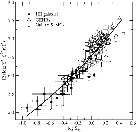
Figure 1: The calculated sulphur abundance for the objects of the sample versus the S₂₃ parameter. The thick line represents the quadratic fit of the points.

After the advent of the ISO mission, it has also been possible to obtain data of the [SIV] at 10.52 $\mu$ emission line for a selected sample of objects, thus allowing the derivation of the S³⁺/H⁺ ionic abundance ratio. We have collected data for 11 HII regions (plus one supernova remnant) in the Large and Small Magellanic Clouds (Vermeij et al., 2002) and for the HII galaxy Mrk209 (Nollenberg et al., 2002). For all these objects the $S^{3+}$ ionic abundances have been recalculated following the procedure described above and using the most recent atomic coefficients from Saraph & Storey (1999). The calculated abundances are listed in table 3.

It has been a matter of debate for some time now what is the exact contribution of the S³⁺/H⁺ ionic abundance to the total abundance of sulphur. It is clear that an efficient solution to this problem could be reached making use of the measurements of the infrared lines of [SIV] –not available for a large sample of objects yet–.

This question takes us straight into the issue of the ionisation correction factor, a necessary step for the derivation of the empirical sulphur abundance calibration. In any case, it has been already pointed out that a one-zone ionisation scheme may provide some insight into the situation for not ionisation bounded HII regions of moderate to low ionisation, where the various ions coexist throughout the nebula (e.g. Pagel 1978). For this reason we have presented above the general correlation between S⁺ + S²⁺ and S₂₃. A study of the ionisation correction factor scheme for sulphur is presented in the next section.

Table 3: Abundances of S³⁺ for the objects for which there are ISO observations of the [SIV] 10.52 $\mu$ emission line and the corresponding ICF(S⁺+S²⁺).

$$\begin{array}[]{cccc}\hline\cr\vskip 3.0pt plus 1.0pt minus 1.0pt\cr Object&Ref.^{a}&12+\log\left(\frac{S^{3+}}{H^{+}}\right)&ICF(S^{+}+S^{2+})\\ \vskip 3.0pt plus 1.0pt minus 1.0pt\cr\hline\cr\\ Mrk209&1&5.93\pm 0.20&1.97\pm 0.62\\ Mrk209^{b}&1&5.68\pm 0.23&1.56\pm 0.76\\ N160-A1&2&6.08\pm 0.11&1.15\pm 0.05\\ N160-A2&2&5.90\pm 0.10&1.11\pm 0.03\\ N159-5&2&6.03\pm 0.10&1.10\pm 0.04\\ N157-B&2&5.54\pm 0.12&1.05\pm 0.02\\ 30Dor-1&2&6.16\pm 0.11&1.27\pm 0.10\\ 30Dor-2&2&6.24\pm 0.11&1.27\pm 0.10\\ 30Dor-3&2&6.16\pm 0.10&1.20\pm 0.06\\ 30Dor-4&2&6.15\pm 0.10&1.23\pm 0.07\\ N83-B&2&5.45\pm 0.12&1.04\pm 0.02\\ N4-A&2&6.17\pm 0.15&1.24\pm 0.11\\ N88-A&2&5.80\pm 0.10&1.75\pm 0.27\\ N66&2&5.73\pm 0.15&1.32\pm 0.19\\ N81&2&5.45\pm 0.11&1.17\pm 0.07\\ \hline\cr\vskip 3.0pt plus 1.0pt minus 1.0pt\cr\vskip 3.0pt plus 1.0pt minus 1.0pt\cr\hline\cr\end{array}$$

• The corresponding references for the emission line data of [SIV] at 10.5 $\mu$ are: 1. Nollenberg et al., 2002; 2. Vermeij et al., 2002

• Assumming a constant $S^{3+}/S^{2+}$ ratio from the [SIII] lines in the near-IR from PMD03

3 The ICF Scheme

Perhaps one of the most difficult aspects in the derivation of total abundances is the question of the ionisation correction factor, ICF. The ICF for sulphur accounts for the contribution of the ionic species not detected in the optical. In high excitation nebulae a large fraction of the sulphur can be found in the S³⁺ stage, whose prominent emission lines of [SIV] are observed in the mid-IR at 10.52 $\mu$. Therefore, in order to derive the total abundance of sulphur it is necessary to correct for the presence of S³⁺ in those objects for which there are not observations in the mid-IR, as follows.

$$\frac{N(S)}{N(H)}=ICF(S^{+}+S^{2+})\cdot\frac{N(S^{+}+S^{2+})}{N(H^{+})}=$$

$$=\frac{N(S^{+}+S^{2+}+S^{3+})}{N(S^{+}+S^{2+})}\cdot\frac{N(S^{+}+S^{2+})}{N(H^{+})}$$

The first proposed ICF scheme for sulphur (Peimbert & Costero, 1969) was based on the similarity of the ionisation potentials of O⁺ (35.1 eV) and S²⁺ (34.8 eV)

$$ICF(S^{+}+S^{2+})=\frac{N(O)}{N(O^{+})}$$

Nevertheless, some authors have pointed out that this relation has a strong correlation with the ionisation degree of the nebula (e.g. Barker 1978; Pagel 1978), thus implying an overestimation of the sulphur abundance in nebulae with low electron temperature. Barker (1980) proposed a new relation, based on the photoionisation models of Stasiǹska (1978):

$$ICF(S^{+}+S^{2+})=\left[1-\left(1-\frac{N(O^{+})}{N(O)}\right)^{\alpha}\right]^{-1/\alpha}$$

for which he proposed a value of $\alpha$ = 3. The ICF from Peimbert & Costero corresponds to a value for $\alpha$ = 1 in this expresion. Later, Izotov et al. (1994), based on photoionisation models from Stasiǹska (1990) gave a fit for this ICF that, in fact, is quite similar to the Barker formula for $\alpha$ = 2.

In figure 2 we show our computation of the ICF(S${}^{+}+S^{2+}$) as a function of log ($O^{+}/O$) using the data listed in table 3, for three different values of $\alpha$ =1,2,3. It is apparent in this plot that most points are better matched for $\alpha$ values between 2 and 3. Only one point, corresponding to a HII galaxy (Mrk 209, solid square), shows an ICF for a value of $\alpha$ even lower than 2. Since the $S^{2+}$ abundances obtained from the [SIII] line at 18.71 $\mu$ from the ISO observations from Nollenberg et al. (2002) are much higher than those obtained from the near-IR [SIII] (PMD03), we have recalculated $S^{3+}$ abundances assuming a constant $S^{3+}$/$S^{2+}$ ratio. This value is showed in table 3 and is represented as an open square in figures 2 and 3. Although showing a large error bar, the new value lies within the zone of $\alpha$ between 2 and 3, in better agreement to the values predicted by photo-ionisation models (PMD03).

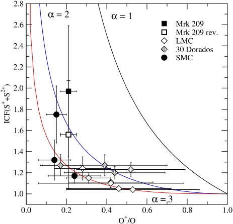
Figure 2: Ionisation correction factor for the sum of $S^{+}$ and $S^{2+}$ versus the $O^{+}/O$ ratio for the sample of objects listed in table 3. The solid lines represent the Barker’s formula for different values of the $\alpha$ parameter. Squares represent different values for Mrk209 (see text for details), diamonds for HII regions in the Large Magellanic Cloud and circles in the Small Magellanic Cloud.

Since the relevant lines for sulphur abundance determination are in the red to near infrared range, it is worth trying to relate the ICF scheme of sulphur to the ionisation structure as seen in this wavelength range. This aproach has the extra bonus of reducing the effect of reddening in the line ratios currently used. In order to derive a new ICF scheme for sulphur based only on the red-to-near infrared information, we need to combine available data and compute new models for reference objects, for which we know all the relevant ionic abundances of sulphur. We have computed this relation and is shown in figure 3. In this plot, we present the ICF(S⁺ + S⁺⁺) vs. log ([SIII]/[SII]) predicted by photo-ionisation models using CoStar model atmospheres of different effective temperatures (35kK, 40kK, 50kK, Pérez-Montero & Díaz, 2005) and HII galaxy models (Pérez-Montero & Díaz, 2004), together with all the observed points available. Clearly, the ICF predicted by a model with a single-star of Teff=35kK is always giving ICF=1 no matter the excitation. The ICF predicted for objects presenting log([SIII]/[SII]) $\leq$0.2 remains small, 1.0$\leq$ICF$\leq$1.05. Above log([SIII]/[SII])=0.4, the ICF model predictions begin to diverge. Up to some point, this behaviour seems to be followed by the data. Giant HII regions points cluster around the locus of 40kK models, except in the notable case of N88A, a SMC reddened, very young HII region breaking out its natal cloud (Heydari-Malayeri et al., 1999). In this plot this giant HII region is located closed to Mrk209, the only HII galaxy in table 3. This fact indicates a hotter ionising source and a larger ICF. It is suggested here that this behaviour could be consistent with the prediction from single burst evolutionary models (e.g. Stasińska et al. 2001) since typically HII galaxies host younger ionizing clusters than giant HII regions (Terlevich et al. 2004). Under this assumption, the equivalent width of H$\alpha$, an age indicator, should provide a useful constraint.

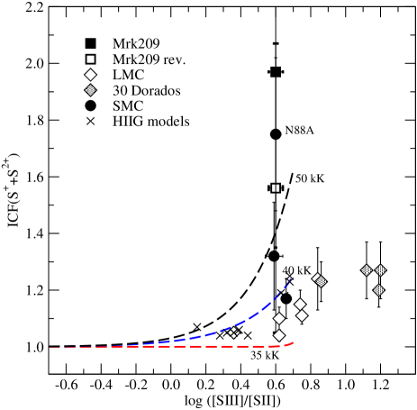
Figure 3: Ionisation correction factor for the sum of $S^{+}$ and $S^{2+}$ versus log ([SIII]/[SII]) for the sample of objects listed in table 3. The dashed lines represent the results from photo-ionisation models for CoStar single star atmospheres with the labelled effective temperature. Crosses represent results from photo-ionisation tailored models of HII galaxies. The rest of symbols are the same as in figure 2.

4 Discussion

Earlier works by Christensen et al. (1997) and by Vermeij et al. (2002) have explored the abundance calibration of S/H versus S₂₃. Christensen et al. (1997) proposed a linear S₂₃ calibration as follows

$$12+\log\left(\frac{S}{H}\right)=6.485+1.218\log S_{23}$$

using data from giant HII regions and HII galaxies available to this date, and complementary model predictions from Stasińska (1990). Though these points included some high metallicity HII regions of M51 from Diaz et al. (1991), as well as lower metallicity objects from Garnett (1992), still the whole abundance range was not sufficiently well sampled. They claimed that more data were needed before a definite conclusion could be drawn.

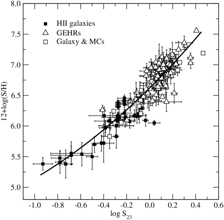
Figure 4: Calculated total sulphur abundance for the objects of the sample versus the S₂₃ parameter. The thick line represents the empirical calibration proposed in this work

Vermeij et al.(2002) derived sulphur abundances for a new data set of optical and infrared spectra of HII regions in the Large and Small Magellanic Clouds. This information allowed these authors to derive all the ionic fractions of sulphur; including S⁺³ from ISO [SIV] 10.5 $\mu$ line for their sample objects. They present a comparison of their S/H abundances points vs. S₂₃ and S₂₃₄ with model calculations for log U = 0, -1, -2, and -3. The following relation was found between log S₂₃ and log(S/H)

$$\log\left(\frac{S}{H}\right)=-5.65+1.50\log S_{234}$$

However no relation was proposed for S/H and S₂₃.

In this work,we present an empirical abundance calibration, based on the bright sulphur lines, which encompasses the whole range of abundance currently found in HII region studies. This calibration is firmly based on an extended homogeneous data base. In figure 4 we present the relation for all the objects of our sample between the S₂₃ parameter and the total abundance of sulphur, taking into account the ionic abundances of S⁺, S²⁺ and the ICF corresponding to the formula of Barker for $\alpha$ = 2.5 which is the value that better fits the available points. The best quadratic fit to the data gives:

$$12+\log\left(\frac{S}{H}\right)=6.622+1.860\log S_{23}+0.382\left(\log S_{23}\right)^{2}$$

with a dispersion of 0.185 dex in the range of -1.0 $\leq$ log(S₂₃) $\leq$ 0.5.

This calibration is, to first order, independent of both, O/H and O₂₃, and is especially suited for observations including only the red to near-infrared spectral ranges (from [SIII]$\lambda$ 6312 Å, H$\alpha$ up to the 1$\mu$ CCD cut-off). Though the S₂₃ parameter is possibly double valued, like R₂₃, the turnover region for S₂₃ is located above the range of sulphur abundance currently found in disk HII regions.

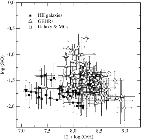
Figure 5: Representation of the quotient of S/O versus O/H for the compiled sample and the solar value

The calibration is, to some extent, affected by the ICF calculation scheme. However only 34% of the objects in our sample show an ICF larger than 1.2 as derived from Barker’s expression ($\alpha$ = 2.5) and all of them show log ([SIII]/[SII]) $>$ 0.4, where model predictions are more uncertain. In fact, the calibration of (S⁺+S²⁺)/H⁺ vs. S₂₃ does not differ much from that of S/H vs. S₂₃ (see figures 1 and 4) and the values obtained from both for a given S₂₃ are within the quoted uncertainty in most cases.

This calibration makes possible the use of S/H as metallicity tracer in ionized nebulae. Its translation however to an O/H abundance relies on the assumption that the S/O ratio remains constant at all abundances. This point though remains controversial (see e.g.Lodders, 2003; Bresolin et al. 2004). Figure 5 shows the S/O ratio vs. 12+log(O/H) for the objects in our sample. For all of them, the O/H abundance has been calculated following the scheme presented in Pérez-Montero & Díaz (2005). It can be seen from the figure that HII galaxy data are consistent with a constant S/O ratio, but significantly lower than the solar ratio. Four galaxies deviate from this trend (UGC4483, KUG 0203-100, Mrk709 and SDSS J1121+0324). One of them, Mrk 709, also shows a large value of N/O (PMD03). Regarding disk HII regions the dispersion is much larger and the assumptions of a constant S/O is highly questionable.

Summarizing, following earlier work by Christensen et al and Vermeij et al, we have derived an empirical calibration of the abundance of S/H as a function of the S₂₃ parameter, defined using bright sulphur lines, which we recommend as a useful tool to derive S/H within a large abundance range of 2 dex, keeping a statistical error of 0.18 dex rms. This abundance range appears well suited to deal with objects from low metallicity HII galaxies to high metallicity HII regions located in the inner parts of the disks of spirals.

- (1) Barker, T. 1978, ApJ, 219, 914.
- (2) Barker, T. 1980, ApJ, 240, 99.
- (3) Bresolin, F., Garnett, D.R. & Kennicutt, R.C. 2004, ApJ, 615, 228.
- (4) Bresolin, F., Schaerer, D., González-Delgado, R. & Stasińska, G. 2005, (accepted by A&A), astro-ph/0506088.
- (5) Castellanos, M., Díaz, A.I. & Terlevich, E. 2002, MNRAS, 329, 315.
- (6) Christensen, T., Petersen, L. & Gammelgaard, P. 1997, A&A, 322, 41.
- (7) Dennefeld, M. & Stasiǹska, G. 1983, A&A, 118, 234.
- (8) De Robertis, M.M., Dufour, R.J. & Hunt, R.W. 1987, JRASC, 81, 195.
- (9) Díaz, A.I. & Pérez-Montero, E. 2000, MNRAS, 312, 130. (DPM00)
- (10) Díaz, A.I., Terlevich, E., Pagel, B.E.J., Vílchez, J.M. & Edmunds, M.G. 1987, MNRAS, 226, 19.
- (11) Díaz, A.I., Terlevich, E., Vílchez, J.M., Pagel, B.E.J. & Edmunds, M.G. 1991, MNRAS, 253, 245.
- (12) Dinerstein, H.L. & Shields, G.A. 1986, ApJ, 311, 45.
- (13) French, H.B. 1980, ApJ, 240, 41.
- (14) Garnett, D.R. 1992, AJ, 103, 1330.
- (15) Garnett, D.R., Dufour, R.J., Peimbert, M., Torres-Peimbert, S., Shields, G.A., Skillman, E.D., Terlevich, E.& Terlevich, R. 1995, ApJ, 449, 77.
- (16) Garnett, D.R. & Kennicutt, R.C., 1994, ApJ, 426, 123.
- (17) Garnett, D.R., Kennicutt, R.C. & Bresolin, F., 2004, ApJ, 607L, 21.
- (18) Garnett, D.R., Shields, G.A., Skillman, E.D., Sagan, S.P. & Dufour, R.J. 1997, ApJ, 469, 93.
- (19) González-Delgado, R.M., Pérez, E., Díaz, A.I., García-Vargas, M.L., Terlevich, E. & Vílchez, J.M. 1995, ApJ, 439, 604.
- (20) González-Delgado, R.M., Pérez, E., Tenorio-Tagle, G., Vílchez, J.M., Terlevich, E., Terlevich, R., Telles, E., Rodríguez-Espinosa, J.M., Mas-Hesse, M., García-Vargas, M.L., Díaz, A.I., Cepa, J. & Casta’neda, H.O., 1994, ApJ, 437, 239.
- (21) Guseva, N.G., Izotov, Y.I. & Thuan, T.X. 2000, ApJ, 531, 776.
- (22) Heydari-Malayeri, M., Charmandaris, V., Deharveng, L, Rosa, M.R. & Zinnecker, H. 1999, A&A, 347, 841.
- (23) Izotov, Y.L., Thuan, T.X. & Lipovetsky, V.A. 1994, ApJ, 435, 647.
- (24) Izotov, Y.L., Thuan, T.X. & Lipovetsky, V.A. 1997, ApJS 108, 11.
- (25) Izotov, Y.L.& Thuan, T.X. 1998, ApJ, 500, 188.
- (26) Kennicutt, R.C., Bresolin, F., French, H. & Martin, P. 2000, ApJ, 537, 589.
- (27) Kennicutt, R.C., Bresolin, F. & Garnett, D.R. 2003, ApJ, 591, 801.
- (28) Kennicutt, R.C. & Garnett, D.R. 1996, ApJ, 456, 504.
- (29) Kinkel, U. & Rosa, M.R. 1994, A&A, 282, 37.
- (30) Kniazev, A,Y, Grebel, E.K., Hao, L., Strauss, M.A., Brinkmann, J. & Fukugita, M. 2003, ApJ, 593, L73.
- (31) Kunth, D. & Sargent, W.L.W. 1983, ApJ, 273, 81.
- (32) Kwitter, K.B. & Aller, L.H. 1981, MNRAS, 195, 939.
- (33) Lequeux, J., Rayo, J.F., Serrano, A., Peimbert, M. & Torres-Peimbert, S. 1979, A&A, 80, 155.
- (34) Lodders, K. 2003, ApJ, 591, 1220.
- (35) Nollenberg, J.G., Skillman, E.D., Garnett, D.R. & Dinerstein, H.L. 2002, ApJ, 581, 1002
- (36) Oey, M.S. & Shields, J.C. 2000, ApJ, 539, 687.
- (37) Pagel, B.E.J., Edmunds, M.G., Blackwell, D.E., Chun, M.S. & Smith, G., 1979, MNRAS, 189, 95.
- (38) Pagel, B.E.J., Simonson, E.A., Terlevich, R.J. & Edmunds, M.G. 1992, MNRAS, 255, 325.
- (39) Pastoriza, M.G., Dottori, H.A., Terlevich, E., Terlevich, R. & D’iaz, A.I. 1993, MNRAS 260, 177.
- (40) Peimbert, M. & Costero, R. 1969, BAAS, 1, 256.
- (41) Peimbert, A., Peimbert, M. & Luridiana, V. 2002, ApJ, 565, 668
- (42) Peimbert, M., Peña, M. & Torres-Peimbert, S. 1986, A&A, 158, 266.
- (43) Pérez-Montero, E. & Díaz, A.I. 2003, MNRAS, 346, 105. (PMD03)
- (44) Pérez-Montero, E. & Díaz, A.I. 2004, ASPC, 322, 213.
- (45) Pérez-Montero, E. & Díaz, A.I. 2005, MNRAS, 361, 1063.
- (46) Saraph, H.E. & Storey, P.J. 1999, A&AS, 134, 369.
- (47) Skillman, E.D., Cø̂té, S. & Miller, B.W. 2003, AJ, 125, 593.
- (48) Skillman, E.D. & Kennicutt, R.C. 1993, ApJ, 411, 655.
- (49) Skillman, E.D., Terlevich, R.J., Kennicutt, R.C.Jr., Garnett, D. & Terlevich, E. 1994, ApJ, 431, 172.
- (50) Stasińska, G. 1978, A&A, 66, 257.
- (51) Stasińska, G. 1990, A&AS, 83, 501.
- (52) Stasińska, G. & Leitherer, C. 1996, ApJS, 107, 661.
- (53) Storey, P.J. & Hummer, D.G. 1995, MNRAS, 272, 41.
- (54) Tayal, S.S. & Gupta, G.P. 1999, ApJ, 526, 541.
- (55) Terlevich, R., Melnick, J., Masegosa, J., Moles, M. & Copetti, M.V.F. 1991, A&AS, 91, 285.
- (56) Terlevich, R., Silich, S., Rosa-González, D. & Terlevich, E. 2004, MNRAS, 348, 1191.
- (57) Vermeij, R., Damour, J.M., van der Hulst, J.M. & Baluteau, J.-P. 2002, A&A, 390, 649.
- (58) Vílchez, J.M. & Esteban, C. 1996, MNRAS, 280, 720.
- (59) Vílchez, J.M., Pagel, B.E.J., Díaz, A.I:, Terlevich, E. & Edmunds, M.G. 1988, MNRAS, 235, 633.