A NOVEL TECHNIQUE FOR WIDE-FIELD POLARIMETRY WITH A RADIOTELESCOPE ARRAY

Abstract

We report the use of the Australia Telescope Compact Array (ATCA) to conduct polarimetric observations of the sky at 5 GHz. The ATCA is normally operated as an interferometer array, but these observations were conducted in a split array mode in which the antenna elements were used as single-dishes with their beams staggered to simultaneously cover a wide area of sky with a resolution of 10$\prime$. The linearly polarized sky radiation was fully characterized from measurements, made over a range of parallactic angles, of the cross correlated signals from the orthogonal linear feeds. We describe the technique and present a polarimetric image of the Vela supernova remnant made as a test of the method. The development of the techniques was motivated by the need for wide-field imaging of the foreground contamination of the polarized component of the cosmic microwave background signal.

1 Introduction

Measurements of the polarized component of the cosmic microwave background (CMBP) are keenly sought to provide an independent measurement of cosmological parameters and verify the precision of certain assumptions that form the basis of cosmological models. Measurements of the CMBP can also give greater insights into both the re-ionization and inflation processes than can be gained from temperature data alone (e.g. Zaldarriaga, Spergel & Seljak, 1997; Kinney, 1999). These measurements are best made at frequencies above 30 GHz and are technically difficult. At any frequency the measurements are expected to suffer from foreground contaminants such as Galactic synchrotron emission and dust (e.g. Tegmark et al., 2000), with the synchrotron emission expected to dominate up to 100 GHz. Observations of Galactic synchrotron emission at lower frequencies will provide a measure of its potential to contaminate the CMBP signal. There have been no polarization surveys of large areas of sky at frequencies above 2.7 GHz (Duncan et al., 1999) and so estimates of contamination at the CMBP observing frequencies currently rely on extrapolations from that frequency and from theoretical considerations (Carretti et al., 2002a). Measurements of sky polarization at shorter centimetre wavelengths would provide useful constraints on that extrapolation. Surveys at higher frequencies have been difficult because of the limited fields of view. In general, the need for wide-field imaging has driven the development of interferometers with smaller array element sizes and single-dish telescopes with receiver arrays at the focal plane. We describe here a novel method of using existing interferometer arrays for wide field imaging. We have used the Australia Telescope Compact Array (ATCA), configured as a set of single-dishes, to make polarimetric observations at 5 GHz. Single-dish radio-polarimetry has not previously been conducted with the ATCA.

The angular power spectrum of the CMB polarization is predicted to peak around spherical harmonic multipoles $\ell=1000$, corresponding to a $\theta\sim 180^{\circ}/\ell\sim 11^{\prime}$ angular scale (Zaldarriaga, Spergel & Seljak, 1997). At 5 GHz (wavelength of 6 cm), the 22-m ATCA antennas have an angular resolution of FWHM $\sim 9^{\prime}$. Therefore, the 22-m ATCA antennas, operating in single-dish total power mode at 5 GHz, are well suited for making a survey of the sky polarization at the multipoles of interest to the planned CMB experiments.

The sky regions that have the lowest dust emission are the Galactic pole areas. However, the minimum Galactic synchrotron emission is observed at lower latitudes ($|b|=40^{\circ}$–50^∘). In particular, a region of interest in the southern sky is at RA $=5^{h}\pm 1^{h}$ Dec $=-45^{\circ}\pm 10^{\circ}$ (Carretti et al., 2002b) which culminates at high elevations at southern mid-latitudes and so is observable with the ATCA antennas with low ground spillover.

We describe the methods used at the ATCA for wide-field radio-polarimetry imaging. The Array’s standard interferometer mode was used to characterize the instrumental errors and calibrate the antenna responses, whereas the wide field imaging was done by using the array in single-dish mode with the pointing of the array elements offset to instantaneously cover a wide sky area. The method has been demonstrated using the ATCA to image the Vela supernova remnant.

2 Method

The ATCA is a six-element aperture synthesis radiotelescope that operates at 20, 13, 6, 3 and 1.2 cm and 3.5 mm (Frater, Brooks & Whiteoak, 1992). Each element is a 22-m antenna with (shaped) Cassegrain optics. Each has three receiver packages that operate over pairs of wavelength bands. Receiver tuning and signal sampling are synchronized across the array by a signal (the local oscillator) distributed from the array centre. A range of signal bandwidths can be selected, and each antenna is equipped to provide two observing bands within the tuning range of the receiver package in use. In this work we have used the 6/3 cm package tuned to two 128 MHz bands centred at 4800 and 4928 MHz. In each band, the signal for each linear polarization is sampled (2-bit) at the Nyquist rate, and transmitted on optical fibres to the digital correlator.

In normal operation the correlator computes the cross-correlation of signal pairs from the array, the two polarizations from each of the six elements yielding 60 cross correlations. These are calibrated and integrated to form the complex visibilities used in aperture synthesis image formation. In addition, autocorrelations and polar cross-correlations are computed for each antenna, and in normal operation are used for calibration. We made use of these correlation products for the single-dish observations described here.

2.1 Single-dish polarimetry

The ATCA antennas are on altitude-azimuth mounts and have two orthogonal linearly polarized feeds $X$ and $Y$ inclined 45^∘ to the vertical. The radiation field incident on the telescope feed has contributions $e$ from the sky, and sources in the immediate environment such as the atmosphere, the antenna and the ground. The stray radiation enters the feed both directly and via a number of reflections off the telescope optics and support structures. Although initially unpolarized, response to this radiation in the $X$ and $Y$ channels may be correlated, resulting in a spurious polarized signal. Let $s$ denote the stray radiation and consider it to be partially polarized. The telescope optics, even for radiation entering along the intended path, is imperfect so there is some leakage of each polarized wave into the other channel. In this section we follow the treatment of radio polarimetry by Hamaker, Bregman & Sault (1996), hereafter HBS96. We describe the leakage with the terms $d_{x}$ and $d_{y}$ and write a leakage matrix $D$ and input vectors $e$ and $s$ as

$$\mbox{\boldmath$D$}=\left(\begin{array}[]{cc}1&d_{x}\\ -d_{y}&1\end{array}\right),\mbox{\boldmath$e$}=\left(\begin{array}[]{cc}e_{x}\\ e_{y}\end{array}\right),\mbox{\boldmath$s$}=\left(\begin{array}[]{cc}s_{x}\\ s_{y}\end{array}\right)$$

The signal entering the receiver is then

$$\mbox{\boldmath$D$}(\mbox{\boldmath$e$}+\mbox{\boldmath$s$})=\left(\begin{array}[]{cc}1&d_{x}\\ -d_{y}&1\end{array}\right)\left(\begin{array}[]{cc}e_{x}+s_{x}\\ e_{y}+s_{y}\end{array}\right)$$

The receiver adds noise ($n_{x}$, $n_{y}$) to each channel and amplifies by gain factors ($g_{x}$, $g_{y}$). Writing

$$\mbox{\boldmath$G$}=\left(\begin{array}[]{cc}g_{x}&0\\ 0&g_{y}\end{array}\right),\mbox{\boldmath$n$}=\left(\begin{array}[]{cc}n_{x}\\ n_{y}\end{array}\right)$$

the input vector $v$ to the correlator is

$$v = \mbox{\boldmath$G$}[\mbox{\boldmath$D$}(\mbox{\boldmath$e$}+\mbox{\boldmath$s$})+\mbox{\boldmath$n$}]$$ (1)

$$= \left(\begin{array}[]{cc}g_{x}&0\\ 0&g_{y}\end{array}\right)\left(\begin{array}[]{cc}e_{x}+s_{x}+n_{x}+d_{x}(e_{y}+s_{y})\\ e_{y}+s_{y}+n_{y}-d_{y}(e_{x}+s_{x})\end{array}\right)$$ (6)

The correlator produces the coherency vector which, in the case of single-dish observations, is the time-averaged outer product (see HBS96) of the input signal with its complex conjugate

$$\mbox{\boldmath$V$}=\left(\begin{array}[]{cc}XX\\ XY\\ YX\\ YY\end{array}\right)=\left<\left(\begin{array}[]{cc}v_{x}v_{x}^{\ast}\\ v_{x}v_{y}^{\ast}\\ v_{y}v_{x}^{\ast}\\ v_{y}v_{y}^{\ast}\end{array}\right)\right>$$ (7)

Then (adopting a convention where $A_{pq}=a_{p}a_{q}^{\ast}$)

$$XX = g_{x}g_{x}^{\ast}[e_{x}e_{x}^{\ast}+s_{x}s_{x}^{\ast}+n_{x}n_{x}^{\ast}+d_{x}(e_{y}e_{x}^{\ast}+s_{y}s_{x}^{\ast})$$

$$\mbox{}+d_{x}^{\ast}(e_{x}e_{y}^{\ast}+s_{x}s_{y}^{\ast})$$

$$\mbox{}+d_{x}d_{x}^{\ast}(e_{y}e_{y}^{\ast}+s_{y}s_{y}^{\ast})]$$

$$= G_{xx}[E_{xx}+S_{xx}+N_{xx}+d_{x}(E_{yx}+S_{yx})$$

$$\mbox{}+d_{x}^{\ast}(E_{xy}+S_{xy})$$

$$\mbox{}+d_{x}d_{x}^{\ast}(E_{yy}+S_{yy})]$$

where the $<>$ symbols are omitted but understood and terms such as $e_{x}s_{x}^{\ast}$ and $s_{x}n_{x}^{\ast}$ are dropped because their factors are uncorrelated and the time-averaged products vanish. Similarly

$$XY = G_{xy}[E_{xy}+S_{xy}+d_{x}(E_{yy}+S_{yy})$$

$$\mbox{}-d_{y}^{\ast}(E_{xx}+S_{xx})$$

$$\mbox{}+d_{x}d_{y}^{\ast}(E_{yx}+S_{yx})]$$

Note that the receiver noise components $n_{x}$ and $n_{y}$ are uncorrelated and so the term $<N_{xy}>$ vanishes and does not appear in the expression for $XY$.

For the ATCA antennas, the leakage terms are stable and easily measured with the Array configured for interferometry. Moreover, they are small ($d\raisebox{-1.29167pt}{\mbox{$\stackrel{{\scriptstyle<}}{{{}_{\sim}}}\,$}}0.03$) and so second order terms ($d_{x}d_{x}^{\ast}$, $d_{x}d_{y}^{\ast}$, etc.) can safely be neglected for this experiment. The components of $V$ are then

$$XX = G_{xx}[E_{xx}+S_{xx}+N_{xx}+d_{x}(E_{yx}+S_{yx})+d_{x}^{\ast}(E_{xy}+S_{xy})]$$ (8)

$$YY = G_{yy}[E_{yy}+S_{yy}+N_{yy}+d_{y}(E_{xy}+S_{xy})+d_{y}^{\ast}(E_{yx}+S_{yx})]$$ (9)

$$XY = G_{xy}[E_{xy}+S_{xy}+d_{x}(E_{yy}+S_{yy})-d_{y}^{\ast}(E_{xx}+S_{xx})]$$ (10)

$$YX = XY^{\ast}$$ (11)

The quantities of interest are the Stokes characterisation of the astronomical signal and can be related to the terms in ($e_{x}$,$e_{y}$) in the expressions above as (see HBS96)

$$E_{xx} = \frac{I+Q^{\prime}}{2}$$ (12)

$$E_{xy} = \frac{U^{\prime}+iV}{2}$$ (13)

$$E_{yx} = \frac{U^{\prime}-iV}{2}$$ (14)

$$E_{yy} = \frac{I-Q^{\prime}}{2}$$ (15)

We seek to measure the linearly polarized sky emission which is characterized by $Q$ and $U$. In Equations 7–10 we use the primed symbols $Q^{\prime}$ and $U^{\prime}$ to emphasize that these are the linear Stokes parameters in the frame of the antenna feeds, not the required $Q$ and $U$ defined relative to the cardinal direction on the sky which must be determined by rotation through the parallactic angle $\psi$ later in the analysis. Expressed as equivalent temperatures, the typical size of the terms in Equations 3–6 for the parameters of our observations are

$$E_{xx} \simeq E_{yy}\;\simeq\;5\mbox{K}$$

$$S_{xx} \simeq S_{yy}\;\simeq\;5\mbox{K}$$

$$N_{xx} \simeq N_{yy}\;\simeq\;25\mbox{K}$$

$$E_{xy} \simeq {E_{xx}-E_{yy}\over 2}\;\simeq\;0.001\mbox{K}$$

It can be seen that $U^{\prime}$ can be determined from $XY$, the component containing terms in $E_{xy}$, whereas the determination of $Q^{\prime}$ involves the difference $XX-YY$. Thus any fluctuations or errors in the determination of the receiver gain will, when multiplied by the large terms in Equations 3 and 4, produce large uncertainties in the value of $Q^{\prime}$. For this reason single-dish radio polarimetry is best performed with feeds receptive to opposite hands of circular polarization so that all the uncertainties arising from differencing the parallel handed components of the coherency vector ($RR$, $LL$) flow into the circular Stokes $V$ component which is often of less astrophysical interest than the linear polarization. Radio interferometry is protected from this because both the stray radiation $s$ and the receiver noise $n$ entering the two antennas of each interferometer are uncorrelated. Thus the ATCA can successfully use linear feeds for polarimetric interferometry. For this experiment, the uncertainties in $Q^{\prime}$ are intolerable and so we must determine the full linear polarization state from measurements of $U^{\prime}$ made at several parallactic angles. This process is described in section 2.4.

Further practical difficulties arise from the stray radiation which is partially polarized and is a strong function of antenna elevation, and also has some azimuthal dependency. These dependencies have proven impossible to model and so all our observations have been conducted as “drift scans”, in which the antennas are held at a fixed azimuth and elevation, and the measurements are recorded as the sky drifts past at the sidereal rate.

The analysis above does not include the possibility of further additive components of stray signal in the polarized outputs. Examples are the components arising from coupling of receiver noise between the two polarizations in the orthomode transducerr, and from common mode noise from the use of common Local Oscillators in the frequency conversion stages of the receiver. These are expected to be constant, independent of antenna pointing, but are difficult to model. Consequently absolute measurements of the polarized emission are not attempted. All observations are differential, with images of the polarized emission being presented after the subtraction of a baseline from each scan.

2.2 ATCA amplitude calibration

At the digitisation stage prior to correlation, the receiver output signals are normalized. At the ATCA, the correlator measures correlation coefficients (which take values in the range [-1,1]) and to recover the absolute scaling of the coherence measurements a calibration system continously measures and records the system temperature $T_{sys}$ of each polarization channel against a noise signal of known temperature $T_{cal}$ which is injected at 45^∘ to the $X$,$Y$ feeds. Typically $T_{cal}\simeq 2\mbox{K}$ referred to the face of the feed horn. The calibration noise signal is switched and a synchronous demodulator measures the signal power $p$ and $q$ during the off and on phases respectively. Let $\sigma$ be the measurement error on the normalized correlator outputs

$$\sigma=\frac{\Delta V^{\prime}_{i}}{V^{\prime}_{i}}\simeq\frac{1}{\sqrt{\tau B}}$$ (16)

where $\tau$ and $B$ are the integration time and signal bandwidth, respectively. A factor $G$ can then be used to scale the normalised correlator outputs

$$\mbox{\boldmath$V$}=G\mbox{\boldmath$V^{\prime}$}=\frac{T_{cal}}{q-p}\mbox{\boldmath$V^{\prime}$}$$ (17)

The measurement error $V$ has contributions from the error $\Delta G$ in the determination of $G$ and from the noise $\sigma$ on the normalized correlator outputs

$$\frac{\Delta G}{G}=\left[\frac{\Delta(q-p)}{q-p}\right]\\$$ (18)

The quantities $p$ and $q$ are independent, being formed by integrating the signal over distinct time intervals $\tau/2$. Let $f=T_{cal}/T_{sys}$. Then $q=p(1+f)$ and

$$\Delta p = \sqrt{2}\sigma p$$

$$\Delta q = \sqrt{2}\sigma q=\sqrt{2}\sigma p(1+f)$$

$$\Delta(q-p) = \sqrt{(\Delta q)^{2}+(\Delta p)^{2}}$$

$$= 2\sigma p\sqrt{1+f+f^{2}/2}$$

$$\frac{\Delta(q-p)}{q-p} = \frac{2\sigma\sqrt{1+f+f^{2}/2}}{f}$$ (19)

Since at the ATCA $f\simeq 0.05$, the errors in the $V_{i}$ are dominated by the error in the determination of $G$

$$\frac{\Delta V_{i}}{V_{i}} \simeq \frac{2\sigma\sqrt{1+f}}{f}$$ (20)

$$\simeq 40\sigma\;\mbox{\hskip 50.00008ptwhen $f=0.05$}$$

Thus, the application of the online $T_{sys}$ calibration increases the noise in $V$ by a factor of about $2/f$ and for this experiment severely limits the sensitivity of the measurements. In addition, since the calibration signal is injected at $45^{\circ}$ to the $X$,$Y$ feeds, it appears as an additional strong polarized component in Equation 5 which, when multiplied by uncertainties and fluctuations in $G_{xy}$ could overwhelm the polarized signal from the sky. Our observations were made with the online application of $T_{cal}$ scaling disabled. The scaling factor $G$ was determined independently from separate integrations that bracketted the observations of the sky.

Note that the difference in the instrumental path lengths for the $X$ and $Y$ polarizations is expected to be non-zero, and antenna specific but only slowly changing. Failing to account for it rotates the signal between Stokes $U$ and $V$. We measured this path-length (phase) difference for each antenna by measuring the phase of the calibration signal that is injected at $45^{\circ}$ to the $X$,$Y$ feeds. The phase correction was then applied to the measured $XY$ values.

2.3 Observational procedure

To measure the polarized emission from a $\Delta\alpha\times\Delta\delta$ rectangular patch of sky centred at $(\alpha,\delta)$ we performed a series of drift scans of duration $\Delta t=\Delta\alpha/\cos\delta$, with the six antennas pointed at the same hour angle and each offset in declination from the next by half the width of the primary beam $\theta$. In successive scans the declination was incremented by $3\theta$ and the hour angle changed (by approximately $\Delta t$) to scan the same range of right ascensions. The entire patch was covered after

$n_{s}=\Delta\delta/3\theta$

scans, and then repeated for the required total integration time. In this way each point in the surveyed area was measured at intervals of approximately

$$n_{s}\Delta t=\frac{\Delta\alpha\Delta\delta}{3\theta\cos\delta}$$

2.4 Determination of $Q$ and $U$

As described in section 2.1, the ATCA is able to provide only one correlated output of the linear polarization Stokes parameters, $U^{\prime}$. Thus $Q$ and $U$ (components defined in sky coordinates) must be constructed starting from this single quantity $U^{\prime}$ by performing at least two scans at parallactic angles $\psi$ ideally differing by $\pm 45^{\circ}$.

The general case consists of $N$ observations of the same pixel performed at several parallactic angles. The two Stokes parameters are estimated through a least square approach. Let ${\tilde{U}^{\prime}}_{i}$ be the $i^{th}$ observation of $U^{\prime}$. Its expression in terms of the actual $Q$ and $U$ values of the sky in the standard reference frame is

$${\tilde{U}}^{\prime}_{i}=-Q\,\sin(2\,\psi_{i})+U\,\cos(2\,\psi_{i}).$$ (21)

where $\psi_{i}$ is the parallactic angle during the observation. (In Equation 17, $\psi_{i}=p_{i}-\phi$ where $p_{i}$ is the parallactic angle and $\phi$ is the fixed angle between the feeds and the vertical-horizontal directions. At the ATCA $\phi=45^{\circ}$.) Minimizing the sum of the square differences

$$S^{2}=\sum_{i}\left({\tilde{U}}^{\prime}_{i}-U^{\prime}_{i}\right)^{2}$$ (22)

with respect to both $Q$ and $U$, we obtain as best estimates

$$Q = {\sum_{i}{\tilde{U}}^{\prime}_{i}\,\sin(2\,\psi_{i})\sum_{i}\cos^{2}(2\,\psi_{i})-\sum_{i}{\tilde{U}}^{\prime}_{i}\,\cos(2\,\psi_{i})\sum_{i}\sin(2\,\psi_{i})\cos(2\,\psi_{i})\over\left(\sum_{i}\sin(2\,\psi_{i})\cos(2\,\psi_{i})\right)^{2}-\sum_{i}\sin^{2}(2\,\psi_{i})\sum_{i}\cos^{2}(2\,\psi_{i})}$$ (23)

$$U = {\sum_{i}{\tilde{U}}^{\prime}_{i}\,\sin(2\,\psi_{i})\sum_{i}\sin(2\,\psi_{i})\cos(2\,\psi_{i})-\sum_{i}{\tilde{U}}^{\prime}_{i}\,\cos(2\,\psi_{i})\sum_{i}\sin^{2}(2\,\psi_{i})\over\left(\sum_{i}\sin(2\,\psi_{i})\cos(2\,\psi_{i})\right)^{2}-\sum_{i}\sin^{2}(2\,\psi_{i})\sum_{i}\cos^{2}(2\,\psi_{i})}$$ (24)

whose errors, assuming all the samplings have the same sensitivity $\sigma_{i}$, are

$${\sigma^{2}_{Q}/\sigma_{i}^{2}} = {\sum_{i}\sin^{2}(2\,\psi_{i})\left[\sum_{i}\cos^{2}(2\,\psi_{i})\right]^{2}-\sum_{i}\cos^{2}(2\,\psi_{i})\left[\sum_{i}\sin(2\,\psi_{i})\cos(2\,\psi_{i})\right]^{2}\over\left[\left(\sum_{i}\sin(2\,\psi_{i})\cos(2\,\psi_{i})\right)^{2}-\sum_{i}\sin^{2}(2\,\psi_{i})\sum_{i}\cos^{2}(2\,\psi_{i})\right]^{2}}$$ (25)

$${\sigma^{2}_{U}/\sigma_{i}^{2}} = {-\sum_{i}\sin^{2}(2\,\psi_{i})\left[\sum_{i}\sin(2\,\psi_{i})\cos(2\,\psi_{i})\right]^{2}+\sum_{i}\cos^{2}(2\,\psi_{i})\left[\sum_{i}\sin^{2}(2\,\psi_{i})\right]^{2}\over\left[\left(\sum_{i}\sin(2\,\psi_{i})\cos(2\,\psi_{i})\right)^{2}-\sum_{i}\sin^{2}(2\,\psi_{i})\sum_{i}\cos^{2}(2\,\psi_{i})\right]^{2}}$$ (26)

giving the fractional errors with respect to the sensitivity of a single observation.

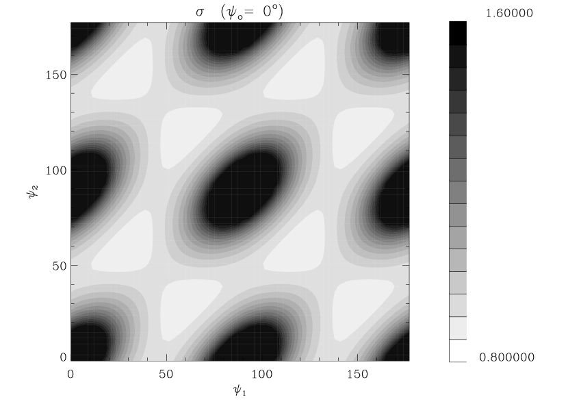
Figure 1: Behaviour of the errors $\sigma/\sigma_{i}$ for the case with $N=3$: The value of $\psi_{0}$ is kept constant, while $\psi_{1}$ and $\psi_{2}$ vary over the range 0^∘ to 180^∘.

These errors depend on the set of parallactic angles at which the measurements occur. The efficiency of the reconstruction thus depends on the scanning strategy adopted, which must be optimized to minimize the error on both $Q$ and $U$. Considering that the method provides two Stokes parameters from measurements of only one, the ideal sensitivity for $N$ observations is

$${\sigma^{\rm th}_{Q,U}\over\sigma_{i}}=\sqrt{2\over N}.$$ (27)

Its comparison with Equations (25) and (26) allows a quantitative estimate of how well $Q$ and $U$ are measured. In addition, to evaluate the overall effect on the ($Q$, $U$) pair, we introduce the mean error

$${\sigma\over\sigma_{i}}=\sqrt{{1\over 2}{\sigma_{Q}^{2}+\sigma_{U}^{2}\over\sigma_{i}^{2}}}.$$ (28)

For the simplest case with N=2 observations, the best result is obtained when the difference ${\rm\psi}_{1}-{\rm\psi}_{0}=\pm\,45^{\circ}$, as expected.

The case N=3 is less trivial. Keeping in mind the ideal value ($\sigma/\sigma_{i}=0.82$ for $N=3$), the case is clear looking at Figure 1, where $\psi_{0}$ is kept constant, while the other two angles $\psi_{1}$ and $\psi_{2}$ are allowed to vary in the 0^∘–180^∘ range. The best sensitivity occurs when the three angles are evenly separated in a $90^{\circ}$ interval, rather than differing by $45^{\circ}$. The case with $\pm 45^{\circ}$ separations favours one of the two Stokes parameters, resulting in a non-optimal combined sensitivity $\sigma$. In general, the optimum result from $N$ observations is obtained with the $90^{\circ}$ range sampled with equally spaced parallactic angles.

3 Test observations

To provide some confidence in the method, we observed $3.5\times 3.0$ degree region centred on the Vela supernova remnant for about 10 hr. This region emits strong polarized emission and has been well studied at a range of wavelengths and resolutions. Milne (1980, 1995) reported polarimetric observations of the Vela nebula at 2.7GHz (resolution 8.4 arcminutes), 5.0 GHz (4.4 arcminutes) and 8.4 GHz (3 arcminutes). Duncan et al. (1997) measured the polarized emission from the southern Galactic plane at 2.4 GHz (resolution 10.4 arcminutes), including the Vela region.

We observed the area with repeated 20-minute drift scans. Each scan was started with all antennas set to $\alpha=08^{h}27^{m}$ and declinations spaced by 5 arcminutes. Thus each scan sampled a 0.5 degree declination band, and six scans were required to sample the whole area. The six scans were repeated for 10 hr, allowing each point in the surveyed area to be measured four or five times. The scan data were reduced to form the image shown in Fig. 2. As described in section 2.2, the ATCA flux scale is referred to a switched noise signal, the “on-line $T_{sys}$ measurement”. The total intensity image was derived from those measurements. The full recovery of $Q$ and $U$ required each point to be measured at different parallactic angles (see section 2.4). In this case the south-west corner of the surveyed area was observed five times at parallactic angles of $-117$, $-96$, $-85$, $-70$ and $-48$ degrees.

Figure 2 shows the resulting image of the Vela supernova remnant. The peak total and polarized intensities are 1.3 K and 0.19 K respectively. The image has a resolution of 12 arcmin. Our image compares well with published data and verifies our techniques for surveying an area in single-dish mode with series of drift scans and the complete measurement of Stokes $Q$ and $U$ through sampling a range of parallactic angles. In particular there is a good match of the polarization position angles between our results and those of Milne (1980, 1995). This indicates successful removal of the polarization offsets and background polarization which, as reported by Milne (1980) is low relative to the polarization of the nebula itself.

The high brightness of the Vela region makes our test image less useful for assessing the ultimate sensitivity of the method and its ability to measure the weak CMBP foregrounds. The apparent noise in the $Q$ and $U$ images of $\sigma_{Q,U}\simeq 3\mbox{~{}mK}$ is dominated by the variations in polarized emission over the field. However, we have made preliminary observations of a region near $\alpha=5^{\rm h}$, $\delta=-49^{\circ}$ at high Galactic latitude, which is expected to have low foreground emission. This is the region chosen for a number of CMBP measurements (e.g. BaR-SPOrt, Cortiglioni et al. 2003, BOOMERanG-B2K, Masi et al. 2005). We made the high-latitude observations using the same method described above for the Vela supernova remnant and used a total bandwidth of $\sim$200 MHz. The results of the completed 5 GHz ATCA observations of this region will be the subject of a future report, in which we will compare them with equivalent measurements at lower frequencies. Reducing the preliminary measurements to determine the sensitivity of a single telescope over a 1-s integration we find $\sigma_{Q}=5.8$ and $\sigma_{U}=5.3\mbox{~{}mK s}^{1/2}$, about a factor of 1.6 greater than expected from an ideal noise analysis. We can estimate the sensitivity to $Q$ and $U$ for a survey area of $\Omega$ with angular resolution $\Delta\Omega$ using $n_{t}$ telescopes as

$$\sigma_{Q,U}\simeq\frac{5.5}{\sqrt{n_{t}T\Delta\Omega/\Omega}}\mbox{~{}mK s}^{1/2}$$ (29)

where $T$ is the total integration time for the survey. For example a 10-hour observation using all six ATCA telescopes should yield $\sigma_{Q,U}\simeq 0.06\mbox{ mK}$ for a survey area of 1 deg² and a resolution of 12$\prime$. This sensitivity would allow a 3$\sigma$ detection of the expected 5 GHz signal of $\sim$0.2 mK (see Carretti et al. (2005) for measurements of the polarized foreground at 2.3 GHz).

Figure 2: The Vela supernova remnant at 4.9 GHz. The image has a resolution of 12$\prime$ (indicated at lower left). The 4.9 GHz data were combined with the published 2.4 GHz image (Duncan et al., 1997) to determine the rotation measure across the nebula, and thus the intrinsic polarization position angles. Total intensity is shown as contours (0.06, 0.10, 0.17, 0.27, 0.44, 0.72, and 1.16 K), polarized intensity and magnetic field direction are shown as line segment lengths and angles, respectively. The scale of the line segment lengths is indicated by the segment at lower left which is equivalent to 0.19 K.

4 Summary

We have described a novel method, and its demonstration, of using an existing interferometer array for wide field imaging. The interferometer mode of observing was used to derive the instrumental calibration and a single-dish observing mode with pointing offsets between the array elements was used for the wide field observing. We used the one correlated output ($U^{\prime}$) to construct both $Q$ and $U$ by observing all points in the imaged area at several parallactic angles. We recognise this as a potential technique for all-sky surveying or monitoring with future radio telescope arrays such as the Square Kilimetre Array (SKA) if the array elements are chosen to have limited sky coverage. This could relax the constraint that the SKA must be built with wide-field elements and allow more conventional parabolic dishes to be used as the SKA elements.

References

- Carretti et al. (2002a) Carretti, E., et al., 2002a in Astrophysical Polarized Backgrounds, AIP Conf. Proc., 609, 109
- Carretti et al. (2002b) Carretti, E., et al., 2002b, in Experimental Cosmology at Millimeter Wavelengths, AIP Conf. Proc., 616, 140
- Carretti et al. (2005) Carretti, E. and McConnell, D. and McClure-Griffiths, N. M. and Bernardi, G. and Cortiglioni, S. and Poppi, S., 2005, MNRAS, 360, L10
- Cortiglioni et al. (2003) Cortiglioni S., et al., 2003, in Warmbein B., ed., 16th ESA Symposium on European Rocket and Balloon Programmes and Related Research, ESA Proc. SP-530, p. 271
- Duncan et al. (1997) Duncan, A.R., Haynes, R.F., Jones, K.L., Stewart, R.T., 1997, MNRAS, 291, 279
- Duncan et al. (1999) Duncan, A.R., Reich, P., Reich, W., Fürst, E., 1999, A&A, 350, 447
- Frater, Brooks & Whiteoak (1992) Frater, R.H., Brooks, J.W., Whiteoak, J.B., 1992, Journal of Electrical and Electronics Engineering, Australia – IE Aust. & IREE Aust., 12, 103
- Hamaker, Bregman & Sault (1996) Hamaker, J.P., Bregman, J.D., Sault, R.J., 1996, A&ASS, 117, 137
- Kinney (1999) Kinney, W.H., 1999, Phys. Rev. D, 58, id. 123506
- Masi et al. (2005) Masi S., et al., 2006, A&A, submitted, astro-ph/0507509
- Milne (1980) Milne, D.K., 1980, A&A, 81, 293-301
- Milne (1995) Milne, D.K., 1995, MNRAS, 277, 1435-1442
- Tegmark et al. (2000) Tegmark, M., Eisenstein D.J., Hu W., de Oliveira-Costa, A., 2000, ApJ, 530, 133-165
- Zaldarriaga, Spergel & Seljak (1997) Zaldarriaga, M., Spergel, D.N., Seljak, U., 1997, ApJ, 488, 1