A Classical Treatment of Island Cosmology

Abstract

Computing the perturbation spectrum in the recently proposed Island Cosmology remains an open problem. In this paper we present a classical computation of the perturbations generated in this scenario by assuming that the NEC-violating field behaves as a classical phantom field. Using an exactly-solvable potential, we show that the model generates a scale-invariant spectrum of scalar perturbations, as well as a scale-invariant spectrum of gravitational waves. The scalar perturbations can have sufficient amplitude to seed cosmological structure, while the gravitational waves have a vastly diminished amplitude.

I Introduction

Recent cosmological obervations CMBresults1 seem to be consistent with the hypothesis that we live in a flat $\Lambda$-dominated Universe seeded by primordial fluctuations that were predominantly adiabatic and nearly scale-invariant. The most successful class of models leading to such a Universe are the Inflationary models guthinflation (see, for instance riotto , brandenberger1 , liddlelyth and langlois for recent reviews).

Recently a new cosmological model has been proposed in Ref. islands called Island Cosmology. In this scenario, the presently observed state of the Universe (i.e., inflating with a cosmological constant), is considered to be the eternal state. Large-scale explosive events which involve local violations of the Null Energy Condition (NEC) lead to the formation of “islands” of matter, one of which is our observed universe. The cause of these explosive events is attributed to quantum fluctuations in some field. While a complete calculation of density perturbations in this scenario (which would require a proper treatment of the back reaction in quantum gravity) is not attempted, the authors show that any other free scalar field responding to the metric fluctuation would produce a scale-invariant spectrum.

In this paper we consider a special version of Island Cosmology where we model the behavior of matter during the NEC-violating event as a classical phantom field in order to compute the perturbation spectrum. The different stages of our model are described below (see Fig. 1):

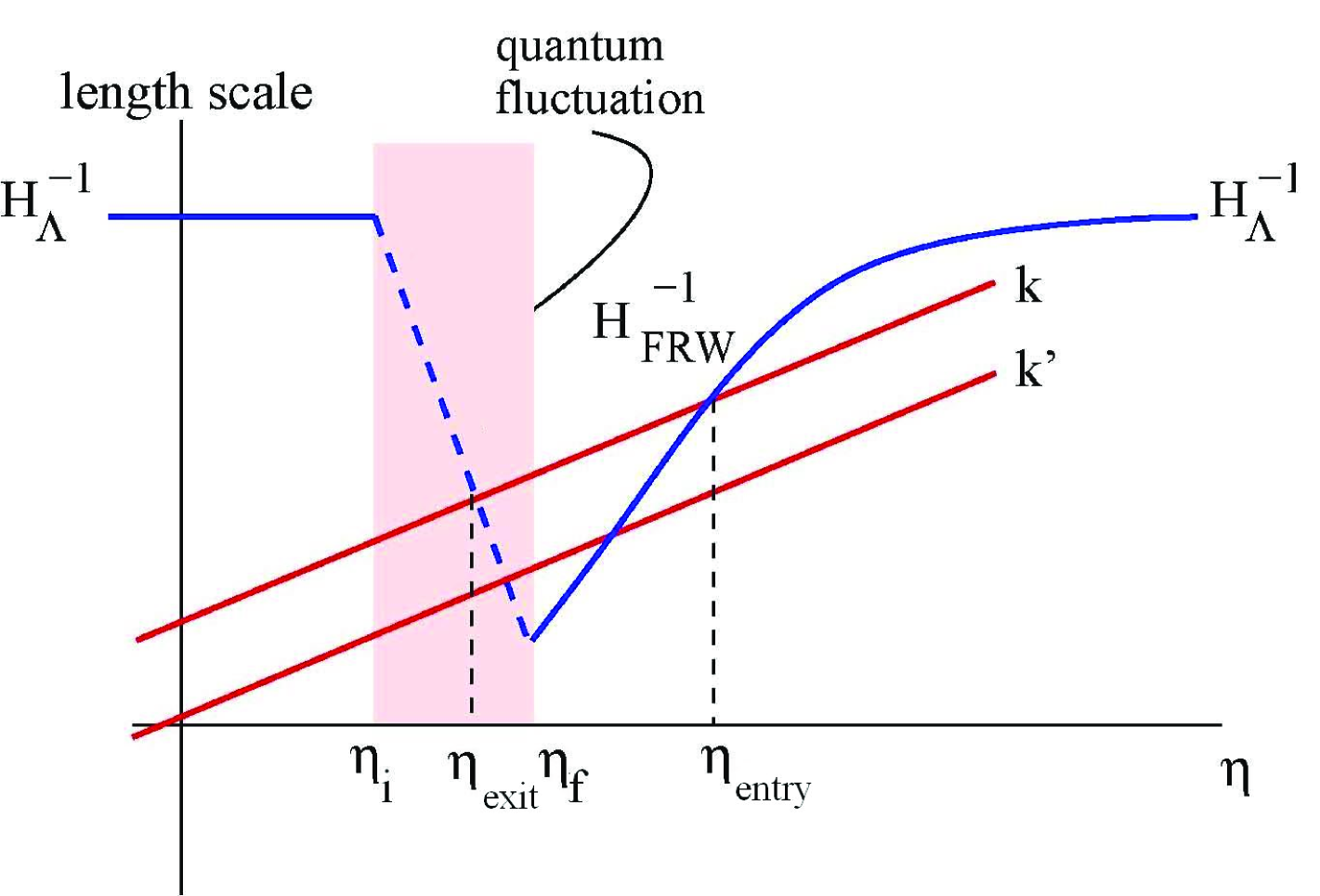
Figure 1: Sketch of the behavior of the Hubble length scale with conformal time, $\eta$, in the Island model, and the evolution of fluctuation modes. At early times, inflation is driven by the presently observed dark energy, assumed to be a cosmological constant. As the cosmological constant is very small, the Hubble length scale is very large – of order the present horizon size. Exponential inflation in some horizon volume ends not due to the decay of the vacuum energy as in inflationary scenarios but due to a quantum fluctuation in the time interval $(\eta_{i},\eta_{f})$ that violates the null energy condition (NEC). The NEC violating quantum fluctuation causes the Hubble length scale to decrease. After the fluctuation is over, the universe enters radiation dominated FRW expansion, and the Hubble length scale grows with time. The physical wavelength of a quantum fluctuation mode starts out less than $H^{-1}_{\Lambda}$ at some early time $\eta_{i}$. The mode exits the cosmological horizon during the NEC violating fluctuation ($\eta_{\text{exit}}$) and then re-enters the horizon at some later epoch ($\eta_{\text{entry}}$) during the FRW epoch (The modes are drawn as straight lines for illustrative purposes only, they actually grow in proportion to the scale factor).

1. The de Sitter Phase: We start with the assumption that the initial state of the Universe is de Sitter space inflating with the currently observed value of the Hubble constant.

2. The Phantom Phase: A quantum fluctuation in some field (chosen to be a light scalar field for simplicity) in the expanding phase of de-Sitter spacetime, and occuring over a Horizon-sized volume drives the Hubble constant to a high value. Such a fluctuation necessarily violates the Null Energy Condition within this volume. In this treatment we make the working hypothesis that during this phase the energy content within a (current) Hubble sized volume of the Universe behaves like phantom energy, i.e., a classical perfect fluid with equation of state $w=p/\rho<-1$, where $p$ and $\rho$ stand for pressure and density respectively, and $\rho>0$. The Hubble length decreases sharply during this period, though the Universe keeps expanding.

3. The FRW Phase: After the explosive event, the Hubble constant is large, and classical radiation fills the volume. Rapid interactions thermalize this radiation, and this part of the Universe then follows a radiation-dominated FRW evolution leading to the Universe that is observed today.

4. The Dilution Phase: Eventually cosmic expansion dilutes out this aggregation of matter, and the volume of space is restored to its initial de Sitter state.

In the remainder of this paper we will show that this model predicts a (nearly) scale invariant spectrum of scalar perturbations with amplitude sufficient to seed structure, as well as a scale invariant spectrum of tensor perturbations of considerably smaller amplitude.

A similar situation was studied by Y.S. Piao in Ref. piao using a different calculational approach.

The layout of the paper is as follows: Section II describes the model in greater detail. Section III discusses the assumptions and outlines our calculational strategy. Section IV presents a detailed calculation of both the scalar and tensor power spectra, and Section V summarizes our findings.

II The Model

In the following subsections, we describe in more detail the three stages of the model, stating the assumptions involved in each stage.

We set our notation as follows: let us choose our cosmic time coordinate $t$ such that the phantom phase (described in Section II.2) begins at $t=t_{i}=0$. In this paper we find it more convenient to work in conformal time ($\eta$) where $dt=a(\eta)\,d\eta$ and $\eta$ ranges between $(-\infty\text{,}\ 0)$ as $t$ goes from $-\infty$ to $+\infty$. We set our conformal time coordinates such that the period of phantom cosmology lasts between $\eta=\eta_{i}=-1/H_{\Lambda}$ and $\eta=\eta_{f}$. The above choices of $t_{i}$ and $\eta_{i}$ are arbitrary and for convenience. Primes denote derivatives with respect to conformal time, and dots denote derivatives with respect to cosmic time. We adopt the convention that the suffix $i$ denotes the value of a quantity at $\eta=\eta_{i}$ and the suffix $f$ denotes the value at $\eta=\eta_{f}$.

II.1 The de Sitter phase

This phase represents the initial state of the Universe, before the onset of the phantom behavior. In this phase, we assume that the Universe is de Sitter space inflating due to the observed dark energy, which we assume is a cosmological constant. The Hubble parameter ($H$) has the same value that it has today, which we call $H_{\Lambda}$ . This expanding de Sitter background can be part of a classical de Sitter spacetime with no beginning and no end, with early contraction and then expansion. We will only consider the expanding phase of the de Sitter spacetime in the following discussion.

We assume that the matter content of the Universe is a classical scalar field ($\phi$) having a Lagrangian $\cal L$ given by:

$${\cal L}=\lambda\partial^{\mu}(\phi)\partial_{\mu}(\phi)-V(\phi)$$ (1)

and a stress tensor given by:

$$T_{\mu\nu}=\lambda\partial_{\mu}(\phi)\partial_{\nu}(\phi)-g_{\mu\nu}{\cal L}$$ (2)

$g^{\mu\nu}$ represent the components of the metric, and $V(\phi)$ represents the potential. For the sake of generality, we have inserted the constant $\lambda$ which determines the sign of the kinetic term. Obviously, $\lambda=+1$ for an ordinary classical scalar field, and $\lambda=-1$ for a phantom field.

The equation of motion of the field is the Klien Gordon equation:

$$\lambda\frac{1}{\sqrt{-g}}\partial_{\mu}\left(\sqrt{-g}g^{\mu\nu}\partial_{\nu}\phi\right)+\frac{\partial V}{\partial\phi}=0$$ (3)

The scale factor $a(t)$ and Hubble value $H(t)$ during this period can be written as follows:

For $(-\infty<t\leq t_{i}=0)$:

$$a(t) = e^{H_{\Lambda}t}$$ (4)

$$H(t) = \frac{\dot{a}(t)}{a(t)}=H_{\Lambda}$$ (5)

In terms of conformal time, for $(-\infty<\eta\leq\eta_{i})$:

$$a(\eta) = -\frac{1}{\eta H_{\Lambda}}$$ (6)

$${\cal H}(\eta) = \frac{a^{\prime}(\eta)}{a(\eta)}=-\frac{1}{\eta}$$ (7)

II.2 The Phantom Phase

In this phase, lasting between the times $\eta_{i}$ and $\eta_{f}$, the Universe undergoes an NEC-violating quantum fluctuation. We model this phase by assuming that the matter content of the Universe behaves like a phantom field $\phi_{p}$ for the duration of the fluctuation.

We assume that this hypothetical phantom field $\phi_{p}$ is classical, i.e., its Lagrangian and stress tensor are given by Eq. (1) and Eq. (2), and it satisfies the Klien Gordon equation Eq. (3).

Using the above equations, one can readily determine the pressure $p$ and energy density $\rho$ of the field. These work out to:

$$p= \frac{1}{3}\sum T_{ii} =\lambda\frac{\phi_{p}^{\prime 2}}{2}-a^{2}(\eta)V(\phi_{p})$$ (8)

$$\rho= T_{00} =\lambda\frac{\phi_{p}^{\prime 2}}{2}+a^{2}(\eta)V(\phi_{p})$$ (9)

Clearly, $p+\rho=\lambda\phi_{p}^{2}$ indicating, as one would expect, that the NEC is violated during this period if our matter field is phantom $(\lambda=-1)$.

Also during this phase, the Hubble horizon size drops from $H^{-1}_{\Lambda}$ to $H^{-1}_{f}$. We assume that this drop is linear in cosmic time, ending at time $t_{f}$. The validity of this assumption, as well as its implications on the matter content of the Universe are discussed later. Thus,

$$H^{-1}(t)=H^{-1}_{\Lambda}-\alpha t\ \text{(for $0\leq t\leq t_{f}$)}$$ (10)

Here $\alpha$ is a dimensionless parameter measuring the rate at which the horizon size changes during the phantom phase. We assume that the quantum fluctuation is very abrupt, and hence $\alpha$ is very large.

Using the definition of conformal time, it is easy to deduce that during this phase ($\eta_{i}\leq\eta\leq\eta_{f}$),

$$a(\eta) = [-\alpha-H_{\Lambda}(1+\alpha)\eta]^{-\frac{1}{1+\alpha}}$$ (11)

$${\cal H}(\eta) = \frac{a^{\prime}(\eta)}{a(\eta)}=\frac{H_{\Lambda}}{[-\alpha-H_{\Lambda}(1+\alpha)\eta]}$$ (12)

$$H(\eta) = \frac{{\cal H}(\eta)}{a(\eta)}=H_{\Lambda}\left[a(\eta)\right]^{\alpha}$$ (13)

We also need to address the nature of the back-reaction of matter on geometry. Let us make the working hypothesis that the back-reaction is fully described by the Friedmann equation.

The actual time duration of this phase can be calculated by demanding continuity of the Hubble value at $t=t_{f}$ (or equivalently, $\eta=\eta_{f}$). Thus we require (see Eq. (13)),

$$H(\eta_{f})=H_{f}$$ (14)

Solving the above equation for $\eta_{f}$, we obtain

$$\eta_{f}=\frac{1}{H_{\Lambda}(1+\alpha)}\left[-\left(\frac{H_{\Lambda}}{H_{f}}\right)^{1+\frac{1}{\alpha}}-\alpha\right]$$ (15)

We assume that $H_{f}\gg H_{\Lambda}$ and since $\alpha\rightarrow\infty$, the first term in the square brackets can be ignored leaving us

$$\eta_{f}\simeq-\frac{\alpha}{H_{\Lambda}(1+\alpha)}-O\left[\frac{1}{(1+\alpha)H_{f}}\right]$$ (16)

From this we can compute the duration of the phantom phase in conformal time ($\Delta\eta$), as follows:

$$\Delta\eta =\eta_{f}-\eta_{i}$$

$$=\frac{1}{H_{\Lambda}}\left(\frac{1}{\alpha+1}\right)$$ (17)

Again, since $\alpha\rightarrow\infty$, this is a vanishingly small interval.

II.3 The Radiation Dominated FRW Phase

In this epoch we have a volume of space of Hubble length $H_{f}^{-1}$ filled with classical radiation. Rapid interactions thermalize the radiation, after which this volume follows a standard FRW evolution.

The scale factor in this radiation-dominated epoch can therefore be written as

$$a(t)=a_{f}\sqrt{\frac{t}{t_{f}}}$$ (18)

In terms of the conformal time, this reduces to

$$a(\eta)=a_{f}+a_{f}^{2}H_{f}(\eta-\eta_{f})$$ (19)

III Calculational Strategy

We make two key assumptions to facilitate our calculation, which we discuss below. These are:

1. During the NEC-violating explosive event the energy content of the Universe behaves as a phantom field.

2. During the NEC violation, the drop in the Hubble scale is linear in cosmic time.

Assumption (1) is an attempt to model the behavior of the matter field during the NEC-violating event. To calculate density fluctuations due to fluctuations in the NEC-violating field, one needs a suitable model for the evolution of the field itself during the NEC-violating fluctuation. This evolution is quantum and not described as a solution to some classical equation of motion. For the purpose of this calculation, we have made the simplifying assumption that the matter field behaves in the same manner as a classical object that would also violate the NEC and produce the same effect on the spacetime. Of course this purely classical treatment cannot substitute for a rigorous quantum mechanical treatment of the NEC-violation, but we hope that it captures the essential elements of the physics involved.

Assumption (2) can be justified considering that the drop in the Hubble length need not be linear throughout the explosive event, but only during the window of time $\delta t$ that it takes for the scales observed today to leave the horizon. Since the fluctuation itself is very short lived, the drop in $H^{-1}(t)$ over $\delta t$ can be well approximated to be linear.

We now turn our attention to computing the spectrum of perturbations that would be generated in this cosmological model. Our plan of action is the following:

1. Working in $k$ (momentum or wavenumber) space, we first find expressions for the Mukhanov variable $v_{k}(\eta)$ in all the three stages of the model. The Mukhanov variable is a gauge-invariant linear combination of matter and metric perturbations representing the true dynamical degrees of freedom of the system. It is fully described in Mukhanov .

2. The unknown coefficients that arise in the above expressions are then determined by demanding continuity of $v_{k}(\eta)$ and its time derivative $v_{k}^{\prime}(\eta)$ at transition times $\eta_{i}$ and $\eta_{f}$.

3. The adiabatic density perturbation responsible for structure in the Universe is conveniently characterized by the curvature perturbation $\cal R$ seen by comoving observers. Once we fully determine $v_{k}(\eta)$ in the radiation dominated phase, we obtain the co-moving curvature perturbation spectrum from the relation (see, for example, liddlelyth )

   $${\cal P}_{\cal R}(\eta)=\frac{k^{3}}{2\pi^{2}}\left|\frac{v_{k}(\eta)}{z(\eta)}\right|_{\text{FRW}}^{2}$$ (20)

   $z$ being defined by the relation

   $$z=a\frac{\phi^{\prime}}{\cal H}$$ (21)

IV The Perturbation Spectrum

In the next three subsections (IV.1, IV.2 and IV.3), we find expressions for $v_{k}$ in the three stages of the model. The unknown coefficients are determined in IV.4, and the scalar and tensor power spectra are computed in IV.5 and IV.6 respectively.

IV.1 $v_{k}$ in the de Sitter Phase

For a scalar field in de Sitter space, the gauge-invariant Mukhanov variable $v_{k}(\eta)$ can be shown to satisfy the equation (see, for instance, langlois )

$$v_{k}^{\prime\prime}(\eta)+\left[k^{2}-\frac{a^{\prime\prime}(\eta)}{a(\eta)}\right]v_{k}(\eta)=0$$ (22)

The solutions to this equation are the Bunch-Davies mode functions:

$$v_{k}(\eta)=\frac{e^{-ik\eta}}{\sqrt{2k}}\left(1-\frac{i}{k\eta}\right)$$ (23)

IV.2 $v_{k}$ in the Phantom Phase

In this case we will calculate $v_{k}$ starting from first principles.

IV.2.1 Matter and metric perturbations

The first step is to perturb the matter and metric. Working in longitudinal gauge and assuming no anisotropic stress, the scalar metric perturbations are written as:

$$g_{\mu\nu}=a^{2}\left(\begin{array}[]{cccc}1+2\Phi&0&0&0\\ 0&-1+2\Phi&0&0\\ 0&0&-1+2\Phi&0\\ 0&0&0&-1+2\Phi\end{array}\right)$$ (24)

Given our choice of gauge, the metric perturbation $\Phi(\eta,\vec{x})$ coincides with the gauge-invariant Bardeen potential (see, for example Mukhanov ).

The phantom matter field $\phi_{p}(\eta,\vec{x})$ is perturbed as follows:

$$\phi_{p}(\eta,\vec{x})=\phi(\eta)+\delta\phi(\vec{x},\eta)$$ (25)

IV.2.2 Evolution of the perturbations

To find time evolution of the perturbations, we use the perturbed Einstein equations up to first order. The i-i component of the zero-th order equations reads:

$$-\Lambda a^{2}+\left(\frac{a^{\prime}}{a}\right)^{2}-2\frac{a^{\prime\prime}}{a}=8\pi G\left[\lambda\frac{\phi^{\prime 2}}{2}-a^{2}V(\phi)\right]\\$$ (26)

while the 0-0 component reads:

$$\Lambda a^{2}+3\left(\frac{a^{\prime}}{a}\right)^{2}=8\pi G\left[\lambda\frac{\phi^{\prime 2}}{2}+a^{2}V(\phi)\right]$$ (27)

Adding these equations, one obtains the familiar relationship:

$${\cal H}^{2}-{\cal H}^{\prime}=4\pi G\lambda\phi^{\prime 2}$$ (28)

The i-i, 0-0 and 0-i components of the first order equations are respectively:

$$\Lambda a^{2}\Phi-2\Phi\left(\frac{a^{\prime}}{a}\right)^{2}+4\Phi\frac{a^{\prime\prime}}{a}+3\frac{a^{\prime}}{a}\Phi^{\prime}+\Phi^{\prime\prime}=$$

$$8\pi G\left[a^{2}V(\phi)\Phi-\frac{1}{2}a^{2}V_{\phi}\delta\phi+\frac{1}{2}\lambda\phi^{\prime}\delta\phi^{\prime}-\lambda\Phi\phi^{\prime 2}\right]$$ (29)

$$\Lambda a^{2}\Phi-3\frac{a^{\prime}}{a}\Phi^{\prime}+\nabla^{2}\Phi=$$

$$8\pi G\left[a^{2}V(\phi)\Phi+\frac{1}{2}a^{2}V_{\phi}\delta\phi+\frac{1}{2}\lambda\phi^{\prime}\delta\phi^{\prime}\right]$$ (30)

$$\Phi^{\prime}+\frac{a^{\prime}}{a}\Phi=4\pi G\lambda\phi^{\prime}\delta\phi$$ (31)

(where $V_{\phi}=\partial V/\partial\phi$).

Perturbing the Klein-Gordon equation Eq. (3) using Eq. (25) yields, at zero-th order:

$$\lambda\left[\phi^{\prime\prime}+2{\cal H}\phi^{\prime}\right]=-a^{2}V_{\phi}$$ (32)

Using Eq. (28), Eq. (29), Eq. (30), Eq. (31) and Eq. (32), one obtains the equation of motion of $\Phi(\eta,\vec{x})$:

$$\Phi^{\prime\prime}-\nabla^{2}\Phi+2\left({\cal H}-\frac{\phi^{\prime\prime}}{\phi^{\prime}}\right)\Phi^{\prime}+2\left({\cal H}^{\prime}-{\cal H}\frac{\phi^{\prime\prime}}{\phi^{\prime}}\right)\Phi=0$$ (33)

Applying the Fourier transform:

$$\Phi(\vec{x},\eta)=\int\frac{d^{3}\vec{k}}{(2\pi)^{3/2}}\,\Phi_{k}(\eta)\,e^{i\vec{k}.\vec{x}}$$ (34)

we obtain:

$$\Phi^{\prime\prime}_{k}+2\left({\cal H}-\frac{\phi^{\prime\prime}}{\phi^{\prime}}\right)\Phi^{\prime}_{k}+\left[k^{2}+2\left({\cal H}^{\prime}-{\cal H}\frac{\phi^{\prime\prime}}{\phi^{\prime}}\right)\right]\Phi_{k}=0$$ (35)

Note that Eq. (35) is independent of $\lambda$, indicating that it has the same form for a phantom field as it would for a normal field. This is a surprising result, since all the equations used to derive Eq. (35) are $\lambda$ dependent. Physically, this result implies that the evolution of the metric perturbation is insensitive to whether the matter content of the Universe is normal or phantom.

To solve Eq. (35), we need to determine the dynamics of the phantom field $\phi(\eta)$, which is in turn determined by the potential $V(\phi)$. We choose a particular form of the potential which allows for a solution in closed form:

$$V(\phi_{p})=K^{2}\frac{(3+\alpha)}{2\alpha}\,\exp\left[\frac{2\alpha H_{\Lambda}}{K}\phi_{p}\right]$$ (36)

Here $K$ is a constant that has the dimensions of mass squared, and sets the scale of the potential.

For this potential, it is easy to verify that the exact form of $\phi(\eta)$ which satisfies Eq. (32) (with of course $\lambda=-1$ as is the case in the phantom phase) is:

$$\phi(\eta)=-\frac{K}{H_{\Lambda}(1+\alpha)}\,\ln\left[-\alpha-H_{\Lambda}(1+\alpha)\eta\right]$$ (37)

Further, to facilitate the back-reaction as discussed in Section II.2, and satisfy our ansatz given by Eq. (10) we must require that our field satisfies the Friedmann equation Eq. (27). The result of this is to fix the value of $K$:

$$K=H_{\Lambda}\sqrt{\frac{3\alpha}{4\pi G}}$$ (38)

The matter field $\phi(\eta)$ has the interesting property that

$$\frac{\phi^{\prime\prime}(\eta)}{\phi^{\prime}(\eta)}=\left(1+\alpha\right){\cal H}(\eta)$$ (39)

Using Eq. (39), Eq. (35) reduces to

$$\Phi_{k}^{\prime\prime}-2{\cal H}\alpha\Phi_{k}^{\prime}+\left[k^{2}-2{\cal H}^{2}\alpha\right]\Phi_{k}=0$$ (40)

This is a familiar second order differential equation of the form:

$$\Phi_{k}^{\prime\prime}+P(\eta)\Phi_{k}^{\prime}+Q(\eta)\Phi_{k}=0$$ (41)

with

$$P(\eta) = -2{\cal H}(\eta)\alpha$$

$$Q(\eta) = k^{2}-2{\cal H}^{2}(\eta)\alpha$$

which has the solution (see e.g. wiesstein )

$$\Phi_{k}(\eta)=e^{-\frac{1}{2}\int P(\eta)\,d\eta}\chi(\eta)=a^{\alpha}\chi(\eta)$$ (42)

where $\chi(\eta)$ satisfies the differential equation

$$\chi^{\prime\prime}(\eta)+\left[Q-\frac{1}{2}P^{\prime}-\frac{1}{4}P^{2}\right]\chi(\eta)=0$$ (43)

In our case, this reduces to

$$\chi^{\prime\prime}(\eta)+\left[k^{2}+\frac{\alpha H_{\Lambda}^{2}}{\left[\alpha+H_{\Lambda}(1+\alpha)\eta\right]^{2}}\right]\chi(\eta)=0$$ (44)

At this point it is convenient to temporarily switch to a new time variable $x$ defined by

$$x=\alpha+H_{\Lambda}(1+\alpha)\eta$$ (45)

Note that $x=-1$ when $\eta=\eta_{i}$ and from Eq. (16), $x=O\left[H_{\Lambda}/H_{f}\right]$ or $x\simeq 0$ when $\eta=\eta_{f}$.

With $x$ as the time variable, Eq. (44) takes the form

$$\frac{d^{2}\chi(x)}{dx^{2}}+\left[m^{2}-\left(p^{2}-\frac{1}{4}\right)\frac{1}{x^{2}}\right]\chi(x)=0$$ (46)

where $m$ and $p$ are defined by

$$m =\frac{k}{H_{\Lambda}(1+\alpha)}$$ (47)

$$p =\left(\frac{1}{4}-\frac{\alpha}{(\alpha+1)^{2}}\right)^{1/2}$$ (48)

The solution to Eq. (46) can be written in terms of Bessel functions as

$$\chi(x)=\sqrt{mx}\left[A_{m}J_{p}(mx)+B_{m}Y_{p}(mx)\right]$$ (49)

where $A_{m}$, $B_{m}$ are constants and $J_{p}$ and $Y_{p}$ denote Bessel functions of the first and second kind of order $p$ respectively.

Putting together Eq. (49) and Eq. (42), we conclude that the time evolution of $\Phi_{k}$ is fully described by the equation

$$\Phi_{k}(\eta)=a^{\alpha}\sqrt{mx}\left[A_{m}J_{p}(mx)+B_{m}Y_{p}(mx)\right]$$ (50)

where $m$, $x$ and $p$ are defined by Eq. (47), Eq. (45) and Eq. (48) respectively, and $\alpha$ is defined in Eq. (10).

IV.2.3 Calculating the Mukhanov Variable

The Mukhanov variable $v_{k}$ can also be defined by the relationship (see, for example brandenberger1 ):

$$v_{k}={\cal R}_{k}z$$ (51)

Where ${\cal R}_{k}$ is the curvature perturbation on co-moving hyper-surfaces at length scale $k$.

We are first going to compute ${\cal R}_{k}$ and then $z$ and then use Eq. (51) to compute $v_{k}$.

Calculation of ${\cal R}_{k}$:

The curvature perturbation on co-moving hyper-surfaces (${\cal R}_{k}$) is defined by the relation (in momentum space) riotto :

$${\cal R}_{k}=\Phi_{k}+{\cal H}\frac{\delta\phi}{\phi^{\prime}}$$ (52)

Noticing that for this space, we have

$$\frac{{\cal H^{\prime}}}{{\cal H}^{2}}-1=\alpha$$ (53)

and using equations Eq. (31) and Eq. (28), we can eliminate the $\delta\phi$ in Eq. (52), giving us an expression for ${\cal R}_{k}$ involving $\Phi_{k}$ and $\Phi^{\prime}_{k}$ as the only first order variables:

$${\cal R}_{k}=\Phi_{k}-\frac{1}{\alpha{\cal H}}\left[\Phi^{\prime}_{k}+{\cal H}\Phi_{k}\right]$$ (54)

(Again, the absence of $\lambda$ indicates that the expression for ${\cal R}_{k}$ is insensitive to whether the field is real or phantom.)

Calculation of $z$:

In the definition of $z$ Eq. (21) we eliminate $\phi^{\prime}$ using Eq. (28), and introduce $\alpha$ using Eq. (53) to get

$$z = a\sqrt{\frac{\alpha}{-4\pi G\lambda}}$$ (55)

$$= am_{\text{Pl}}\sqrt{\frac{2\alpha}{-\lambda}}$$

where $m_{\text{Pl}}$ is the reduced Planck mass defined by $m_{\text{Pl}}=\sqrt{1/8\pi G}$, where $G$ is Newton’s gravitational constant.

Final expression for $v_{k}$:

Combining Eq. (51), Eq. (54) and Eq. (55), we can express $v_{k}$ entirely in terms of $\Phi_{k}$ and $\Phi^{\prime}_{k}$ as follows:

$$v_{k}=a\sqrt{\frac{\alpha}{-4\pi G\lambda}}\left[\Phi_{k}-\frac{1}{\alpha{\cal H}}\left(\Phi^{\prime}_{k}+{\cal H}\Phi_{k}\right)\right]$$ (56)

IV.3 $v_{k}$ in the FRW Phase

Here we have a gauge field in a geometry described by Eq. (19). From the theory of cosmological perturbations, we know that $v_{k}$ satisfies langlois

$$v_{k}^{\prime\prime}(\eta)+\left[k^{2}-\frac{z^{\prime\prime}(\eta)}{z(\eta)}\right]v_{k}(\eta)=0$$ (57)

But since $z(\eta)=2m_{\text{Pl}}a(\eta)$ in this space, the above equation simply reduces to Eq. (22). Solving Eq. (22) for this space, we find that $v_{k}$ is described by the solution:

$$v_{k}(\tau)=\alpha_{k}e^{ik\tau}+\beta_{k}e^{-ik\tau}$$ (58)

where $\alpha_{k}$ and $\beta_{k}$ are constants of integration and $\tau=\eta-\eta_{f}>0$

IV.4 Calculation of Unknown Constants

The above calculations produced four unknown constants $A_{m}$, $B_{m}$, in Eq. (49) and $\alpha_{k}$ and $\beta_{k}$, in Eq. (58). These constants can be determined by demanding continuity of $v_{k}$ and its time derivative at the two transition times $\eta_{i}$ and $\eta_{f}$.

To determine $A_{m}$ and $B_{m}$, we perform the above matching process at $\eta=\eta_{i}=-\frac{1}{H_{\Lambda}}$, or in terms of $x$, (from Eq. (45)), at $x=x_{i}=-1$ . In other words, we need to simultaneously solve the equations

$$v_{k}\text{(de Sitter)}|_{\left(\eta=-1/H_{\Lambda}\right)}=v_{k}\text{(phantom)}|_{(x=-1)}$$

$$v_{k}^{\prime}\text{(de Sitter)}|_{\left(\eta=-1/H_{\Lambda}\right)}=v_{k}^{\prime}\text{(phantom)}|_{(x=-1)}$$ (59)

to find the unknowns $A_{m}$ and $B_{m}$.

The expression obtained for $v_{k}$ in the phantom phase (by substituting the values of the above constants) is fairly complicated. However, since we are only interested in the super-horizon modes, we can make the approximation that $k\text{ (or $m$)}\rightarrow 0$, and use the appropriate asymptotic forms of the Bessel functions $J_{p}(mx)$ and $Y_{p}(mx)$. Also, since $\alpha$ is large, from Eq. (48), $p\simeq\frac{1}{2}$. With these simplifications the expression for $v_{k}$ (in the phantom phase) reduces to:

$$v_{k}(x) \simeq -\frac{i\,e^{ik/H_{\Lambda}}a^{(1+\alpha)}H_{\Lambda}(-1+x\alpha)}{\sqrt{2}k^{3/2}(1+\alpha)}$$ (60)

$$+O\left[k^{-1/2}\right]$$

$$v_{k}^{\prime}(x) \simeq -\frac{i\,e^{ik/H_{\Lambda}}a^{(1+\alpha)}H_{\Lambda}^{2}}{\sqrt{2}k^{3/2}x}+O\left[k^{-1/2}\right]$$ (61)

Now having fully determined the form of $v_{k}(\eta)$ during the phantom phase, we can determine the coefficients $\alpha_{k}$ and $\beta_{k}$ in Eq. (58) to determine $v_{k}(\eta)$ in the final FRW phase. In particular, we need to solve simultaneously the equations:

$$v_{k}\text{(phantom)}|_{\left(x\simeq 0\right)}=v_{k}\text{(FRW)}|_{(\eta=\eta_{f})}$$

$$v_{k}^{\prime}\text{(phantom)}|_{\left(x\simeq 0\right)}=v_{k}^{\prime}\text{(FRW)}|_{(\eta=\eta_{f})}$$ (62)

For brevity, let us call the leading term in $k$ in the expression for $v_{k}$ (Eq. (60)) at $\eta=\eta_{f}$ (or $x\simeq 0$) as $l_{1}$ and the leading term in $k$ in the expression for $v_{k}^{\prime}$ (Eq. (61)) at $x\simeq 0$ as $l_{2}$. Thus we have

$$l_{1}=\frac{i\,e^{ik/H_{\Lambda}}a^{(1+\alpha)}H_{\Lambda}}{\sqrt{2}k^{3/2}(1+\alpha)}$$ (63)

and,

$$l_{2} = -\frac{i\,e^{ik/H_{\Lambda}}a^{(1+\alpha)}H_{\Lambda}^{2}}{\sqrt{2}k^{3/2}x_{f}}$$ (64)

$$= \frac{i\,e^{i/kH_{\Lambda}}a_{f}^{(2+2\alpha)}H_{\Lambda}^{2}}{\sqrt{2}k^{3/2}}$$

Where in the last manipulation we have used the result that $-x_{f}=a_{f}^{-(1+\alpha)}$, which follows from the form of the scale factor during the phantom phase (Eq. (11)) and the definition of $x$ (Eq. (45)). Eq. (62) now implies that

$$\alpha_{k} =\frac{1}{2}\left[l_{1}+\frac{l_{2}}{ik}\right]$$

$$\beta_{k} =\frac{1}{2}\left[l_{1}-\frac{l_{2}}{ik}\right]$$ (65)

Using Eq. (13) at ($\eta=\eta_{f}$) to find

$$a_{f}^{\alpha}H_{\Lambda}=H_{f}$$ (66)

we note from equations Eq. (64) that,

$$\frac{l_{1}}{l_{2}}=\frac{1}{(1+\alpha)a_{f}^{1+\alpha}H_{\Lambda}}=\frac{1}{a_{f}H_{f}(1+\alpha)}\ll 1$$ (67)

since both $\alpha$ and $H_{f}$ are large. Eq. (65) now reduces to

$$\alpha_{k} \simeq \quad\frac{1}{2}\left[\frac{l_{2}}{ik}\right]$$

$$\beta_{k} \simeq \,-\frac{1}{2}\left[\frac{l_{2}}{ik}\right]$$ (68)

Hence the form of $v_{k}(\eta)$ in the phantom phase becomes:

$$v_{k}(\eta) \simeq \frac{l_{2}}{2ik}e^{ik\tau}-\frac{l_{2}}{2ik}e^{-ik\tau}$$ (69)

$$= l_{2}\left(\frac{sin(k\tau)}{k\tau}\right)\tau$$

IV.5 Determination of the Scalar Power Spectrum

Now we are in a position to determine the power spectrum of the co-moving curvature perturbation in the FRW space using Eq. (20) which gives

$${\cal P}_{\cal R}=\frac{k^{3}}{2\pi^{2}}\left|l_{2}\frac{sin(k\tau)}{k\tau}\frac{\tau}{z_{\text{FRW}}(\eta)}\right|^{2}$$ (70)

Making the approximation $a_{\text{FRW}}(\eta)=a_{f}^{2}H_{f}\tau$ from Eq. (19) since at the time a mode re-enters the horizon, $\eta\gg\eta_{f}$, using the relation Eq. (66), and taking the limit $k\rightarrow 0$, we finally obtain

$${\cal P}_{\cal R} \simeq \frac{k^{3}}{2\pi^{2}}\left|\frac{i\,e^{-ik/H_{\Lambda}}}{2\sqrt{2}k^{3/2}m_{\text{Pl}}}H_{f}\right|^{2}$$ (71)

$$= \left(\frac{H_{f}}{4\pi m_{\text{Pl}}}\right)^{2}$$ (72)

Hence we find that our model produces a (nearly) scale invariant spectrum of cosmological perturbations, with amplitude set by $H_{f}/m_{\text{Pl}}$. If we assume $H_{f}\sim 10^{14}\text{ GeV}$ (approximately GUT scale), then the power spectrum matches the COBE DMR observations Smoot of CMB temperature fluctuations of order $10^{-5}$. In other words, the perturbation spectrum can have an amplitude sufficiently large to seed the cosmological structure that we see today.

IV.6 Determination of the Tensor Power Spectrum

We know from the theory of cosmological perturbations (see, for example, langlois ) that gravitational waves are essentially equivalent to two massless scalar fields (for each polarization) up to a renormalization factor of $2/m_{\text{Pl}}$. Hence we can write the tensor power spectrum ${\cal P}_{{\cal R}T}$ as

$${\cal P}_{{\cal R}T}=2\frac{4}{m_{\text{Pl}}^{2}}{\cal P}_{{\cal R}\psi}$$ (73)

where the first factor on the right comes from the two polarization states, the second represents the renormalization mentioned above, and ${\cal P}_{{\cal R}\psi}$ is the spectrum of perturbations of a massless scalar field $\psi$ other than, and not interacting with, the NEC-violating field. The $\psi$-field perturbations can be computed using essentially the same machinery as above, with a small difference in the final step:

1. We solve Eq. (35) with $\psi$ representing the matter field.

2. We find expressions for $v_{k}$ in the three stages of the model (up to constants of integration).

3. We demand the continuity of $v_{k}$ and $v_{k}^{\prime}$ at $\eta_{i}$ and $\eta_{f}$ to fully specify the expression for $v_{k}$ in the FRW region (that is, evaluate the undetermined constants obtained in the previous step), and from this, compute the perturbation spectrum ${\cal P}_{{\cal R}\psi}$ using the relation

   $${\cal P}_{{\cal R}\psi}(\eta)=\frac{k^{3}}{2\pi^{2}}\left|\frac{v_{k}(\eta)}{a(\eta)}\right|_{\text{FRW}}^{2}$$ (74)

The final expression for the power spectrum of tensor perturbations turns out to be

$${\cal P}_{{\cal R}T}=8\left(\frac{H_{\Lambda}}{a_{f}^{3}\pi m_{\text{Pl}}}\right)^{2}\simeq 8\left(\frac{H_{\Lambda}}{\pi m_{\text{Pl}}}\right)^{2}$$ (75)

The last step follows because it is easy to show (by Taylor expanding $a(\eta)$ about the point $\eta=\eta_{i}$) that the scale factor hardly changes from its initial value of $1$ during the NEC-violating event.

This result agrees (up to $O(1)$ numerical factors) with the corresponding result obtained in islands .

A similar scenario was investigated by Y.S Piao piao , and while he obtains a scale invariant spectrum of scalar perturbations, the tensor perturbation spectrum in his calculation turns out to be blue-shifted. The source of the discrepancy could lie in his assumption that the canonical relationship satisfied by $v_{k}$ in the case of the tensor spectrum has a time-dependent mass given by $a^{\prime\prime}(\eta)/a(\eta)$ (Eq. (12) in piao ) during the phantom phase. In our approach we derive $v_{k}$ from first principles and find that the time dependent mass can have a more complicated form.

V Conclusions

To summarize, in this paper we have investigated a cosmological model in which islands of matter are created from NEC-violating explosive events in a cosmological constant dominated inflating Universe. Our approach was to model the behavior of the matter field during the NEC-violating fluctuation as a classical phantom field. While an ideal approach would be a full quantum mechanical calculation, it is hoped that our classical calculation can capture the essential elements of the physics involved.

Our calculations yield, (using an exactly solvable potential), an adiabatic spectrum of scale-invariant perturbations, whose amplitude is determined by the value of the Hubble constant at the end of the NEC-violating fluctuation. If we assume the latter to be approximately GUT scale, the perturbation spectrum turns out to have an amplitude sufficient to seed the cosmological structure seen today. We also obtain a scale-invariant spectrum of gravitational waves of amplitude set by $(H_{\Lambda}/m_{\text{Pl}})$.

The essential elements of Island Cosmology, namely, the $\Lambda$-sea and the scale invariant perturbation spectra, are supported by current observations. The NEC-violating quantum fluctuations which create the matter islands are a clear consequence of the basic formalism of quantum field theory. Island cosmology therefore holds out the tantalizing notion that the observed Universe could have had a purely quantum field theoretic origin. This paper lends further support to this idea.

- (1) D. N. Spergel et al., Astrophys. J. Suppl. 148 (2003) 175 [arXiv: astro-ph/0302209]; C. L. Bennett et al., Astrophys. J. Suppl. 148 (2003) 1 [arXiv: astro-ph/0302207]; S. Perlmutter et al., Nature, 391, 51 (1998); A. G. Riess et al., Astron. J. 116, 1009 (1998); S. Perlmutter et al., Astrophys. J. 517, 565 (1999).
- (2) A. H. Guth, Phys. Rev. D 23, 347 (1981).
- (3) D. H. Lyth and A. R. Liddle, Cosmological Inflation and Large-Scale Structure, Cambridge University Press (2000).
- (4) A. Riotto, arXiv: hep-ph/0210162.
- (5) R. Brandenberger, arXiv: hep-ph/0306071.
- (6) D. Langlois, arXiv: hep-th/0405053.
- (7) Sourish Dutta and Tanmay Vachaspati, Phys. Rev. D 71, 083507 (2005) [arXiv: astro-ph/0302209].
- (8) Y. Piao, arXiv: astro-ph/0506072.
- (9) V. F. Mukhanov, H. A. Feldman and R. H. Brandenberger, Phys. Rept. 215, 203 (1992).
- (10) G. F. Smoot et al., Astrophys. J. 396 (1992) L1;
- (11) P. M. Morse and H. Feshbach, Methods of Theoretical Physics, Part I, McGraw-Hill (1953).