High precision determination of the atmospheric parameters and abundances of the COROT main targets

Abstract

Context. One of the main goals of the COROT mission is to get precise photometric observations of selected bright stars in order to allow the modelling of their interior through asteroseismology. However, in order to interpret the asteroseismological data, the effective temperature, surface gravity, and chemical composition of the stars must be known with sufficient accuracy.

Aims. To carry out this task, we have developed a spectroscopic method called APASS (Atmospheric Parameters and Abundances from Synthetic Spectra) which allows precise analysis of stars with a moderate to high rotational velocity, which is the case for most primary COROT targets.

Methods. Our method is based on synthetic spectra in which individual lines are replaced by analysis units (isolated lines or line blends, depending on the crowding of the spectral region and on the rotational broadening). It works differentially with respect to the Sun and allows the atmospheric parameters and chemical abundances to be determined by considering analysis units with different sensitivities to these various parameters.

Results. Using high signal-to-noise spectra and the APASS method, we determined the atmospheric parameters and chemical abundances of 13 primary COROT targets. Our results agree well with those obtained by Bruntt using his software VWA and with those obtained with the software TEMPLOGG. However, in both cases, our error bars are significantly smaller than those of other methods. Our effective temperatures are also in excellent agreement with those obtained with the IR photometry method. For five stars with relatively low rotational velocity, we also performed an analysis with a classical equivalent–width method to test agreement with APASS results. We show that equivalent–width measurements by Gaussian or Voigt profile–fitting are sensitive to the rotational broadening, leading to systematic errors whenever the projected rotation velocity is non–negligible. The APASS method appears superior in all cases and should thus be preferred.

1 Introduction

COROT (COnvection, ROtation and planetary Transits) will carry out several projects in asteroseismology (Baglin et al., (1998)). It will also be the first satellite launched with the aim of detecting exoplanets by the transit method (Rouan et al., (2000)). The instrument features a 27 cm telescope, and the asteroseismology program will use two 2048$\times$2048 CCD cameras, leading to a field of view of 3.5 deg². During the 2.5 years of the mission, 5 fields of the Galactic plane will be observed continuously, each one during 150 days. Among these fields, a few bright stars have been selected as candidate primary targets of the mission, and getting a precise photometric monitoring of these stars to allow the modelling of their interior is the main goal of the asteroseismological part of COROT (see Table 1 for the preliminary list of these primary targets).

To allow thorough modelling of the stellar interior, asteroseismological data are not enough, so additional constraints must be provided by precisely determining the atmospheric parameters and abundances. To accomplish this task, we set up a spectroscopic analysis method, APASS (Atmospheric Parameters and Abundances from Synthetic Spectra), that aims at the highest possible precision. With this method, we analysed the majority of the COROT main targets, including some stars later rejected from the preliminary main target list.

In Sect. 2, we present the spectroscopic observations used in this work, and in Sect. 3, the method APASS is described. In Sect. 4, we present the results and compare them to previous studies. We give our conclusions in Sect. 5.

Table 1: Preliminary list of COROT main targets from Baglin et al., (2004). The $v$ sin$i$ values were provided by C. Catala (private communication). HD 52265 has a giant planet detected by spectroscopy (Butler et al., (2000)).

Star	Spectral type	$v$ sin$i$ (km s-1)
HD 52265	GO III-IV	5.2
HD 49933	F2 V	10.9
HD 49434	F1 V	89.6
HD 43587	F9 V	5.9
HD 170580	B2 V	16.0	$\beta$ Cep
HD 171834	F3 V	72.1
HD 177552	F1 V	41.2
HD 181555	A5 V	$>$ 200	$\delta$ Scuti
HD 180642	B1.5 II-III		$\beta$ Cep
HD 45067	F8 V	8.0
HD 46558	F0 V	63.1
HD 43318	F6 V	7.5
HD 175726	G5 V	13.5
HD 171234	A3 V	162.8	$\delta$ Scuti

2 Spectroscopic observations

We extracted a spectrum of each of the COROT main targets analysed here from the COROT ground-based asteroseismology database, Gaudi (Solano et al., (2005)). All but one were obtained with the ELODIE spectrograph attached to the 1.93 m telescope at Observatoire de Haute-Provence (OHP). ELODIE is a fiber-fed cross-dispersed Echelle spectrograph that provides a complete spectral coverage of the 3800-6800 $\AA$ region, with a resolving power R = 45000 (Baranne et al., (1996)). The spectrum of HD 52265 was obtained with the CORALIE spectrograph attached to the 1.20 m Swiss telescope at La Silla (Chile), providing a resolving power R = 50000 (Queloz et al., (2000)). For one star, HD 49933, we also made an analysis with a co-addition of $\sim 100$ spectra obtained using the ultra–high resolution (R = 115000) HARPS spectrograph attached to the 3.60 m ESO telescope at La Silla (Mayor et al., (2003)). Table 2 gives the observation log for the spectra used in this analysis.

Table 2: Observation log for the spectra of the stars we analysed. The signal-to-noise ratio ($S/N$) in the last column is calculated around 6500 $\AA$. $co$-$ad$: co-addition of $\sim 100$ spectra taken the same night.

Star	Instrument	Date	UT start	$S/N$
HD 43587	ELODIE	14-Jan-98	22:32	250
HD 57006	ELODIE	10-Dec-00	00:41	250
HD 45067	ELODIE	15-Jan-98	22:20	260
HD 43318	ELODIE	19-Jan-98	22:48	120
HD 49933	ELODIE	21-Jan-98	22:17	210
HD 49933	HARPS	19-Jan-04	$co$-$ad$	750
HD 55057	ELODIE	15-Jan-98	23:10	270
HD 184663	ELODIE	18-Jun-00	01:30	170
HD 49434	ELODIE	17-Jan-98	22:33	160
HD 171834	ELODIE	05-Sep-98	19:00	300
HD 177552	ELODIE	14-Jul-98	22:46	260
HD 175726	ELODIE	10-Jul-01	21:23	140
HD 46558	ELODIE	21-Dec-99	01:08	140
HD 52265	CORALIE	24-Nov-01	08:03	140

3 Description of the method

Using the assumptions of Local Thermodynamic Equilibrium (LTE) and plane-parallel, homogeneous atmosphere, APASS is a differential method based on the synthesis of selected spectral regions with Sun-calibrated line data and comparison with a stellar spectrum in order to determine the projected rotational velocity ($v$ sin$i$), the effective temperature $T_{\rm eff}$, the surface gravity log $g$, the microturbulence velocity $\epsilon_{\rm turb}$, as well as the atmospheric abundances.

3.1 Analysis Units (AnU)

We developed APASS in order to be able to precisely analyse stellar spectra with a moderate to high projected rotational velocity (see Table LABEL:tab:ere), which cannot be analysed with a classical equivalent–width (EW) method. Such spectra are convolved with the rotation profile, and most lines are blended with other ones, forming “packs” of lines. One of the main characteristic of APASS is that it considers either individual lines or “packs” of lines, treating them as analysis units (AnU). Those AnU are selected in the first step of the analysis, by visual inspection of the stellar spectrum. All the AnU that are dominated by iron (iron-dominated AnU : Fe–AnU) are used in determining the atmospheric parameters, while the other AnU are used to determine the atmospheric abundances.

3.2 Atmospheric models

We used models interpolated in the Vienna model atmosphere grid (Nendwich et al., (2003), Nend2 (2004); Heiter et al., (2002)). They were computed with a modified version of the ATLAS9 code (Kurucz, (1993)) in which turbulent convection theory in the CGM formulation (Canuto et al., (1996)) is implemented.

3.3 Atomic data

APASS uses limited spectral regions selected on the basis of the following criteria :

• scarcity of telluric lines,

• absence or scarcity of molecular lines,

• high diversity of atomic lines: different elements, various sensitivities to the atmospheric parameters,

• presence of numerous pseudo-continuum windows to accurately normalize the continuum in order to gain precision.

The atomic lines data were extracted from the VALD database (Kupka et al., (1999); Piskunov et al., (1995); Ryabchikova et al., (1999)) and the Kurucz atomic lines database (Kurucz, (1998)). For all the lines with a significant equivalent–width, we made a new determination of the log $gf$ from an inverted analysis of the Jungfraujoch Solar Atlas (Delbouille et al., (1973)), using a CGM solar model having ($T_{\rm eff}$, log $g$, $\epsilon_{\rm turb}$) = (5778 K, 4.44 dex, 1.00 km s^-1) and solar abundances from Grevesse & Sauval (1998). Whenever possible, we used damping constants calculated following Anstee & O’Mara (Anstee1 (1995)), which have proved to be quite accurate (Anstee et al., (1997); Barklem & O’Mara, (2000)).

3.4 Parameter determination

APASS is an iterative method. Starting from an initial model, the method consists of cycles of determination of the parameters, repeated until convergence for all parameters. Each cycle includes adjusting the continuum, determining the level of convolution of the spectrum, and determining the atmospheric parameters $T_{\rm eff}$, log $g$, $\epsilon_{\rm turb}$, and [Fe/H]. The projected rotational velocity $v$ sin$i$ is determined afterwards.

3.4.1 Initial model

For each star analysed in this work, we begin with an initial atmospheric model computed with parameters $T_{\rm eff}$, log $g$, $\epsilon_{\rm turb}$ and a metallicity extracted from the literature or obtained using Strömgren indices from the Gaudi database and the sofware TEMPLOGG (Rogers, (1995)). To synthesize the spectrum of the selected regions, we also need to set initial values for two parameters representing the convolution of the spectrum:

• the projected rotational velocity $v$ sin$i$. As initial value, we use the $v$ sin$i$ determined by C. Catala (private communication),

• the parameter $\Omega$ representing the combined effect of the instrumental profile and the stellar macroturbulence. We use an initial value of 4 km s^-1 for $\Omega$ and assume a Gaussian shape for that convolution profile.

3.4.2 Correction of the Doppler shift

Before starting the first cycle of parameter determination, we use the synthetic spectrum computed with the initial model to determine the Doppler shift of the stellar spectrum. For this purpose, we select a large number of AnU and determine the ratio of their position in the stellar spectrum and in the synthetic spectrum. We use the average ratio for correcting the spectra that are synthesized afterwards.

3.4.3 Adjustment of the continuum

We begin each cycle with a new determination of the continuum of the observed spectrum on the basis of a number of pseudo-continuum windows selected from inspection of both the observed and synthetic spectra. The mean flux in these windows is measured in both the theoretical and the observed spectra, and a table is constructed that contains the ratios of the mean fluxes. A spline curve is then fitted through these points, and the stellar spectrum is divided by that curve, providing our re-normalized spectrum. This method allows us to take into account the weak lines present in the pseudo–continuum windows as accurately as possible.

3.4.4 Determination of the convolution parameter $\Omega$

The convolution parameter $\Omega$ (macroturbulence + instrumental profile) is determined for every Fe–AnU by adjusting the synthetic spectrum with an $\chi^{2}$ minimization method, and the average overall Fe–AnU is the adopted value for $\Omega$ (see Figure 1). During all iteration cycles, we keep $v$ sin$i$ fixed at its initial value. Indeed, as these two broadening parameters appear to be strongly anticorrelated in an $\chi^{2}$ minimization, allowing both of them to vary produces instabilities in the algorithm.

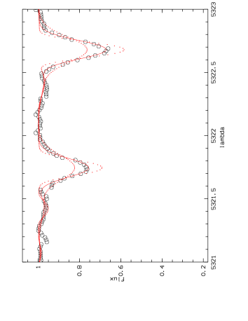
Figure 1: Portion of the stellar spectrum of HD 52265 (empty circles) showing two Fe–AnU. Overplotted: synthetic spectrum computed with $\Omega$ = 0.75 and 6.75 km s^-1 (dotted lines) and with $\Omega$ = 3.75 km s^-1, the best–fit value (continuous line). lambda = wavelength in $\AA$, flux = normalized stellar flux.

3.4.5 Determination of the Fe abundance

A value of the Fe abundance is deduced from each Fe–AnU in the following way. First, the user defines the limits in wavelength of the Fe–AnU considered. Then, the surface under the Fe–AnU is computed in between the two limits of the observed spectrum. This is a kind of “observed EW”. The same is done for the synthetic spectrum. If the two surfaces are not equal, the Fe abundance is modified and a new synthetic spectrum is computed, and so on until the computed surface matches the observed one. The adopted Fe abundance is the average of the values found from all the Fe–AnU considered.

3.4.6 Determination of the atmospheric parameters $\epsilon_{\rm turb}$, $T_{\rm eff}$, and log $g$

In a first step, the sensitivity of each Fe–AnU to the atmospheric parameter considered is determined. First, we deal with the microturbulence velocity $\epsilon_{\rm turb}$. We adopt a value of $\epsilon_{\rm turb}$ and compute the Fe abundance from each Fe–AnU. Then, we change the value of $\epsilon_{\rm turb}$ by a fixed amount and recompute the Fe abundances using this new model. The difference in Fe abundance obtained when changing $\epsilon_{\rm turb}$ gives the sensitivity of each Fe–AnU to this parameter. Once the sensitivity of each Fe–AnU to $\epsilon_{\rm turb}$ is determined, a diagram of abundance versus sensitivity is constructed and $\epsilon_{\rm turb}$ is determined in order to remove any correlation: the deduced abundance should not depend on the sensitivity to $\epsilon_{\rm turb}$. This procedure is similar to the classical method where $\epsilon_{\rm turb}$ is adjusted so that the abundance does not correlate with the line EW (the latter roughly giving the sensitivity to $\epsilon_{\rm turb}$ for weak to medium strength lines). The microturbulence is determined in order to remove any correlation between the abundances and the sensitivities (see Figure 2). In simple words, we want all the Fe–AnU to give us the same global abundance, whatever their sensitivity to $\epsilon_{\rm turb}$.

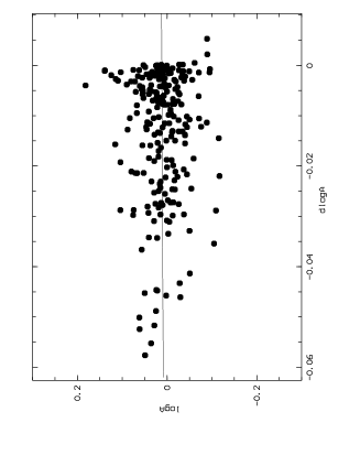
Figure 2: Plot of the abundance deduced from each AnU as a function of the sensitivity of the AnU to $\epsilon_{\rm turb}$ , for $\epsilon_{\rm turb}$ = 1.20 km s^-1 (top) and for $\epsilon_{\rm turb}$ = 1.30 km s^-1 (bottom). The slopes obtained by linear regression are -0.96 $\pm$ 0.24 for $\epsilon_{\rm turb}$ = 1.20 km s^-1 (initial guess) and -0.04 $\pm$ 0.24 for $\epsilon_{\rm turb}$ = 1.30 km s^-1 (adopted value).

Following the same method, the correction to the abundances of our Fe–AnU is computed for two models differing by their value of $T_{\rm eff}$. Once the sensitivity of our Fe–AnU to $T_{\rm eff}$ is computed, $T_{\rm eff}$ is adjusted to remove any correlation between the abundances and the sensitivities to $T_{\rm eff}$, which is similar to removing the trend in the abundance versus line excitation potential plot.

The same method is applied again to determine log $g$; i.e. the sensitivity to log $g$ of the Fe–AnU is computed, and the surface gravity is adjusted to remove any correlation between the abundances and the sensitivities to log $g$.

A complete cycle includes determinations of $\Omega$, [Fe/H], $\epsilon_{\rm turb}$, $T_{\rm eff}$, and log $g$. The iteration ends after convergence, i.e. when the corrections on all parameters become much smaller than the error bars.

3.4.7 Determination of $v$ sin$i$

Once convergence is reached, $v$ sin$i$ is determined by adjusting the synthetic spectrum by an $\chi^{2}$ minimization for every Fe–AnU, and the average value is taken as the final $v$ sin$i$. If this final value significantly differs from the initial value, the whole iteration process is repeated. As mentioned above, $v$ sin$i$ is not adjusted during the iteration cycles because it is strongly anticorrelated with $\Omega$. Adjusting both parameters together thus produces instabilities.

3.5 Computation of the error bars on the parameters

For each parameter, we must distinguish the intrinsic uncertainty and the uncertainties coming from errors on the other parameters (external uncertainties).

3.5.1 Intrinsic uncertainties

For $T_{\rm eff}$, log $g$, and $\epsilon_{\rm turb}$, the standard deviation on the slope in the sensitivity versus abundance of Fe–AnU diagram allows us to compute the intrinsic uncertainty on these parameters, i.e. the statistical deviation. As an example, the uncertainty on the slopes in Figure 2 is 0.24, and the difference between the two slopes is 1.00, for a difference in $\epsilon_{\rm turb}$ = 0.10 km s^-1 between the models. The intrinsic uncertainty on $\epsilon_{\rm turb}$ will be in this case:

$$\sigma=0.10/1.00\times 0.24=0.02\textrm{ km s${}^{-1}$}.$$ (1)

The convolution parameters $v$ sin$i$ and $\Omega$, as well as the iron abundance [Fe/H], are determined independently for each Fe–AnU. The adopted value is the average value for all the Fe–AnU used, and the intrinsic uncertainty is the standard deviation of the mean.

3.5.2 Uncertainty on one parameter due to the intrinsic uncertainty on another parameter

To compute the uncertainties on, e.g., log $g$ coming from another parameter, e.g., $T_{\rm eff}$, we make a new determination of log $g$ using a model with $T_{\rm eff}$ differing from the adopted value by its intrinsic uncertainty. As an example, if we have a final value for log $g$ = 4.34 dex and a final value for $T_{\rm eff}$ = 6400 K with a standard deviation = 50 K, we set $T_{\rm eff}$ to 6450 K (or 6350 K) and determine log $g$. The difference between the obtained value for log $g$ and 4.34 dex is the uncertainty on log $g$ coming from the uncertainty on $T_{\rm eff}$.

For each atmospheric parameter, we compute the uncertainties coming from all the other parameters. The total error bar is then computed as a quadratic sum of these uncertainties. The intrinsic uncertainty is added quadratically to the external uncertainties to obtain the final error bar. An exception exists for $v$ sin$i$, for which we consider the intrinsic uncertainty and the uncertainty coming from $\Omega$ as fully correlated. In this case, the intrinsic uncertainty is added linearly to the uncertainty coming from $\Omega$, and the result is added quadratically to the other uncertainties to obtain the final error bar on $v$ sin$i$.

3.6 Test of the APASS method on an ELODIE spectrum of the Moon

As a test, we determined the parameters of the Sun using an ELODIE spectrum of the sunlight reflected by the Moon. Starting with $T_{\rm eff}=6000$ K, log $g=4.00$ , $\epsilon_{\rm turb}=2.00$, [Fe/H] = 1.00, and $v$ sin$i=5$ km s^-1 as initial guess parameters, the method converged to the following parameters: $T_{\rm eff}=5786\pm 25$ K, log $g=4.45\pm 0.03$, $\epsilon_{\rm turb}=1.01\pm 0.06$ km s^-1 , [Fe/H] = $+0.01\pm 0.02$, and $v$ sin$i=1.94\pm 0.72$ km s^-1. These are very close (and well within error bars) to the “expected” solution, i.e. the set of values used in our solar model: $T_{\rm eff}=5778$ K, log $g=4.44$, $\epsilon_{\rm turb}=1.00$ km s^-1, [Fe/H] = 0.00 , $v$ sin$i=2.00$ km s^-1. This test demonstrates the correct convergence of APASS and the consistency of the ELODIE spectrum with the Jungraujoch Solar Atlas.

3.7 Abundance determination

Once we have obtained the atmospheric parameters, we determine the atmospheric abundances for every element for which we have AnU containing significant lines of this element. We proceed by steps, in order to avoid accumulating the uncertainties. We first adjust the abundance of elements within AnU containing lines of these elements alone or blended only with iron lines. For the sake of clarity, let us call A such an element. Once we have determined the Fe abundance and the abundance of A, we can proceed determining the abundance of an element X whose lines are blended with lines of Fe and A. And so on, until all elements with significant lines are included.

3.8 Computation of the error bars on the abundances

The uncertainty is computed taking into account the part coming from the uncertainty on the abundances of the other elements included in the AnU that we used, along with the uncertainty on the parameters. Let us consider an example. We determine [Si/H] using ten lines, contained in 8 different AnU. The standard deviation of the mean is 0.02 dex. Eight of these lines are blended in their AnU with Fe and Cr lines. We quadratically sum 0.02 dex to the intrinsic dispersion on [Cr/H] and [Fe/H], obtaining e.g. 0.04 dex. Then with different atmospheric models we determine the uncertainties on [Si/H] coming from the intrinsic uncertainties on the atmospheric parameters; i.e. we redetermine [Si/H] with a model whose $T_{\rm eff}$ equal the adopted value plus or minus the intrinsic uncertainty on $T_{\rm eff}$, and we do the same for log $g$, $\epsilon_{\rm turb}$, $\Omega$, and $v$ sin$i$. We then quadratically sum all the uncertainties on [Si/H], obtaining the final error bar. For elements for which we do not have enough AnU to get a significant standard deviation of the mean, we take the average of standard deviations for the other elements except iron. We set to 4 the minimum number of AnU needed to judge the standard deviation significant.

4 Results - comparison

4.1 Stellar parameters

The final stellar parameters are presented in Table 4. The results are compared to other determinations:

• We used the software TEMPLLOG (Rogers, (1995)) and the Strömgren indices extracted from the Gaudi database (Table 3) to determine the atmospheric parameters $T_{\rm eff}$, log $g$, and [Fe/H], with a precision around 200-250 K, 0.3 dex, and 0.2 dex, respectively, according to Rogers. For HD 52265, the H_β index was not available on Gaudi, so we took it from Hauck & Mermilliod (1998).

• For nine of the stars, $T_{\rm eff}$ was determined with the IR photometry method developed by Ribas et al. (Ribas (2003)), considered as more reliable than TEMPLOGG by the COROT team (C. Catala, private communication).

• For the stars HD 43587, HD 43318, HD 45067, HD 57006, and HD 49933, which have a low enough rotation velocity, we also used our equivalent–width method to analyse them. This method is described in Bruntt et al. (2004).

• The star HD 52265 has a massive planet orbiting it that was detected by the radial velocity method (Butler et al., (2000)). Santos et al. derived stellar parameters for planet-host stars using an equivalent–width method (Santos et al., (2004)). For HD 52265, they made two analyses, one based on a CORALIE spectrum and the other on a FEROS spectrum.

• Nine of the stars analysed in this work were also analysed by Bruntt using the VWA software (Bruntt et al., (2002), Bruntt et al., (2004)). This method is based, as is APASS, on the comparison of the stellar spectrum with synthetic spectra.

Figure 3 shows the comparison of our values for $T_{\rm eff}$, log $g$, and [Fe/H] with the values obtained with TEMPLOGG and our equivalent–width method, and with the values obtained by Bruntt with VWA, while Figure 4 shows the comparison of our values for $T_{\rm eff}$ with the values obtained with the IR photometry method.

Table 3: Strömgren photometric indices of the COROT main targets analysed in this work taken from the GAUDI database. The H_β index for HD 52265 is taken from Hauck & Mermilliod (1998)

Star	V	Hβ	(b-y)	m1	c1
HD 52265	6.294	2.619	0.360	0.186	0.423
HD 43587	5.720	2.633	0.382	0.188	0.366
HD 43318	5.629	2.656	0.320	0.154	0.462
HD 45067	5.880	2.638	0.364	0.165	0.405
HD 57006	5.916	2.634	0.336	0.181	0.494
HD 49933	5.782	2.659	0.268	0.133	0.466
HD 175726	6.731	2.621	0.366	0.176	0.312
HD 177552	6.510	2.675	0.243	0.132	0.545
HD 184663	6.430	2.675	0.278	0.149	0.466
HD 46558	6.887	2.736	0.244	0.143	0.542
HD 171834	5.416	2.675	0.250	0.148	0.543
HD 49434	5.753	2.759	0.170	0.181	0.705
HD 55057	5.463	2.742	0.184	0.182	0.877

Table 4: COROT targets and stellar parameters obtained with APASS. HD 49933 was analysed with an ELODIE spectrum (E) and a high $S/N$ HARPS spectrum (H). See text for more details and Table 5 for references.

Star	$v$ sin$i$ (km/s)	$\epsilon_{\rm turb}$ (km s-1)	$T_{\rm eff}$ (K)	log $g$ (dex)	[Fe/H] (dex)	Ref.
HD 52265	$5.0\pm 1.3$	$1.30\pm 0.04$	$6179\pm 18$	$4.36\pm 0.03$	$+0.24\pm 0.02$	1
		$1.33\pm 0.08$	$6131\pm 47$	$4.35\pm 0.13$	$+0.25\pm 0.06$	3
		$1.38\pm 0.09$	$6076\pm 57$	$4.20\pm 0.17$	$+0.20\pm 0.07$	4
			$6135\pm 200$	$4.09\pm 0.20$	$+0.05\pm 0.20$	5
			$6136\pm 51$			7
HD 43587	$5.8\pm 0.9$	$1.18\pm 0.04$	$5978\pm 18$	$4.29\pm 0.02$	$+0.02\pm 0.02$	1
			$5870\pm 60$	$4.20\pm 0.15$	$-0.09\pm 0.11$	6
		$2.13\pm 0.10$	$5867\pm 20$	$4.29\pm 0.06$	$-0.13\pm 0.02$	2a
			$6327\pm 200$	$4.54\pm 0.20$	$+0.24\pm 0.20$	5
			$5925\pm 65$			7
HD 43318	$7.6\pm 2.2$	$1.56\pm 0.08$	$6196\pm 33$	$3.68\pm 0.06$	$-0.16\pm 0.03$	1
			$6190\pm 90$	$3.70\pm 0.15$	$-0.21\pm 0.11$	6
		$2.13\pm 0.31$	$6045\pm 40$	$3.63\pm 0.07$	$-0.24\pm 0.03$	2a
			$6517\pm 200$	$4.25\pm 0.20$	$-0.06\pm 0.20$	5
			$6220\pm 98$			7
HD 45067	$7.9\pm 1.3$	$1.31\pm 0.05$	$6070\pm 23$	$3.99\pm 0.04$	$-0.02\pm 0.02$	1
			$5970\pm 100$	$3.80\pm 0.15$	$-0.17\pm 0.11$	6
		$2.00\pm 0.13$	$5913\pm 30$	$3.91\pm 0.08$	$-0.15\pm 0.02$	2a
			$6358\pm 200$	$4.37\pm 0.20$	$+0.02\pm 0.20$	5
			$6092\pm 59$			7
HD 57006	$8.2\pm 1.5$	$1.68\pm 0.06$	$6177\pm 26$	$3.66\pm 0.05$	$-0.02\pm 0.02$	1
			$6180\pm 70$	$3.60\pm 0.15$	$-0.08\pm 0.11$	6
		$2.72\pm 0.09$	$6026\pm 22$	$3.61\pm 0.05$	$-0.09\pm 0.02$	2a
			$6250\pm 200$	$3.74\pm 0.20$	$+0.06\pm 0.20$	5
HD 49933	$10.3\pm 1.8$	$1.65\pm 0.10$	$6700\pm 65$	$4.25\pm 0.09$	$-0.34\pm 0.03$	1 (E)
	$10.0\pm 1.6$	$1.84\pm 0.08$	$6735\pm 53$	$4.26\pm 0.08$	$-0.37\pm 0.03$	1 (H)
			$6780\pm 70$	$4.30\pm 0.20$	$-0.30\pm 0.11$	6
		$2.53\pm 0.31$	$6467\pm 56$	$4.27\pm 0.08$	$-0.37\pm 0.04$	2a (E)
		$2.12\pm 0.24$	$6539\pm 47$	$4.41\pm 0.07$	$-0.45\pm 0.02$	2a (H)
		$2.33\pm 0.24$	$6538\pm 44$	$4.38\pm 0.08$	$-0.47\pm 0.02$	2b (H)
			$6543\pm 200$	$4.24\pm 0.20$	$-0.38\pm 0.20$	5
			$6747\pm 64$			7
HD 175726	$12.7\pm 1.7$	$1.32\pm 0.08$	$6217\pm 32$	$4.61\pm 0.04$	$+0.03\pm 0.03$	1
			$6227\pm 200$	$4.73\pm 0.20$	$-0.05\pm 0.20$	5
HD 177552	$38.9\pm 2.5$	$1.88\pm 0.10$	$7025\pm 55$	$4.45\pm 0.08$	$-0.03\pm 0.03$	1
			$6657\pm 200$	$4.03\pm 0.20$	$-0.38\pm 0.20$	5
			$7042\pm 69$			7
HD 184663	$57.3\pm 5.3$	$2.01\pm 0.26$	$6511\pm 108$	$4.28\pm 0.21$	$-0.13\pm 0.06$	1
			$6600\pm 90$	$4.50\pm 0.50$	$-0.19\pm 0.21$	6
			$6700\pm 200$	$4.40\pm 0.20$	$-0.13\pm 0.20$	5
HD 46558	$60.0\pm 5.9$	$1.63\pm 0.21$	$7053\pm 92$	$4.44\pm 0.14$	$+0.04\pm 0.07$	1
			$7223\pm 200$	$4.71\pm 0.20$	$-0.24\pm 0.20$	5
			$6922\pm 66$			7
HD 171834	$70.0\pm 6.3$	$1.64\pm 0.21$	$6833\pm 105$	$4.14\pm 0.15$	$+0.01\pm 0.07$	1
			$6840\pm 200$	$4.60\pm 0.50$	$-0.25\pm 0.21$	6
			$6658\pm 200$	$4.04\pm 0.20$	$-0.17\pm 0.20$	5
			$6879\pm 67$			7
HD 49434	$85.4\pm 6.6$	$2.77\pm 0.26$	$7632\pm 126$	$4.43\pm 0.20$	$+0.09\pm 0.07$	1
			$7300\pm 200$	$4.40\pm 0.45$	$-0.04\pm 0.21$	6
			$7343\pm 200$	$4.21\pm 0.20$	$+0.01\pm 0.20$	5
			$7346\pm 69$			7
HD 55057	$130.1\pm 7.5$	$3.20\pm 0.27$	$7478\pm 105$	$3.84\pm 0.17$	$+0.26\pm 0.08$	1
			$7580\pm 250$	$3.60\pm 0.50$	$+0.14\pm 0.21$	6
			$7141\pm 200$	$3.47\pm 0.20$	$+0.08\pm 0.20$	5

Table 5: The references for Table 4

Ref.1	This study with APASS
Ref. 2a	EW method, Kurucz 1993 model
Ref. 2b	EW method, CGM model
Ref. 3	Santos et al. (2004), EROS spectrum
Ref. 4	Santos et al. (2004), CORALIE spectrum
Ref. 5	TEMPLOGG using Strömgren indices from Gaudi database
Ref. 6	Bruntt et al. (2004) using VWA
Ref. 7	IR photometry (Ribas et al., 2003)

Figure 3: Comparison of the atmospheric parameters $T_{\rm eff}$, log $g$ , and [Fe/H], derived in this work with those obtained with our EW method (top), by Bruntt using VWA (middle), and with TEMPLOGG using Strömgren indices from the Gaudi database (bottom).

4.1.1 Comparison with TEMPLOGG values

For $T_{\rm eff}$, we found an average difference $<\delta>$ = -2 K when comparing our values with those obtained with TEMPLOGG. Nevertheless, as can be seen in Figure 3, the dispersion is high ($\sigma=253$ K). Despite the small number of points, a tendency seems to appear in the plot. TEMPLOGG tends to give higher values than APASS for $T_{\rm eff}\sim$ 6000 K, and lower values for higher $T_{\rm eff}$. For log $g$, $<\delta>=-0.03$ dex with $\sigma$ = 0.30 dex, and for [Fe/H] the $<\delta>=+0.07$ dex and $\sigma=0.18$ dex. We thus conclude that our results generally agree with the values obtained with TEMPLOGG. However, the scatter is rather large, and can generally be explained by the larger error bars in the photometric TEMPLOGG determination.

4.1.2 Comparison with IR photometry values

As can be seen from Figure 4, agreement between the $T_{\rm eff}$ obtained with APASS and from IR photometry is very good, within the small error bars for most of the stars: $<\delta>=+40$ K, with $\sigma=110$ K. Only the hottest star, HD 49434, shows significant disagreement. If we do not consider it, $<\delta>$ is reduced to +9 K and $\sigma$ to 55 K.

Figure 4: Comparison of the $T_{\rm eff}$ derived in this work with those obtained with the IR photometry method of Ribas et al. (2003).

4.1.3 Comparison with the values obtained with our EW method

We find $<\delta>=+167$ K with $\sigma=187$ K for $T_{\rm eff}$, when comparing our results using APASS with those obtained using our EW method. The values obtained for [Fe/H] ($<\delta>=+0.09$ dex, $\sigma=0.11$ dex) and for $\epsilon_{\rm turb}$ ($<\delta>=-0.75$ km/s, $\sigma=0.86$ km/s) are not in very good agreement either. Only the values obtained for log $g$ are consistent ($<\delta>=0.00$ dex, $\sigma=0.08$ dex).

Our EW method uses Gaussian and Voigt profile–fitting to measure the EW of single lines. All the stars analysed here have a $v$ sin$i$ higher than the Sun, and we wanted to know if the measured EW are independent of the rotational broadening. We measured the EW of three synthetic FeI lines computed with different convolution parameters $v$ sin$i$, with solar values for $\epsilon_{\rm turb}$, $T_{\rm eff}$, log $g$, and [Fe/H] and with a fixed value of $\Omega$. We also computed the theorical equivalent–width of these lines. Our results in Figure 5 show that the measured EW is sensitive to the rotational broadening of the lines. The fit of Gaussian profiles tends to give EW values that are too low for low $v$ sin$i$, and the measured EW tends to increase with $v$ sin$i$. The fit of Voigt profiles gave good results for low values of $v$ sin$i$, but seemed to give absolutely incorrect values for values of $v$ sin$i$ higher than 4 km/s. The same test with a fixed value of $v$ sin$i$ and different values of $\Omega$ showed also a clear dependence of the measured EW on the convolution magnitude of the spectrum.

We plot in Figure 6 the observed differences between the two methods as a function of $v$ sin$i$. For $T_{\rm eff}$, a clear tendency appears. The higher the rotational broadening of the spectrum, the larger the discrepancy between the 2 methods, with the EW method giving values lower than APASS. For the other parameters, we can only say that lower [Fe/H] and higher $\epsilon_{\rm turb}$ are found with the EW method. All those results seem to indicate that an EW method using Gaussian and Voigt profiles fitting is not suitable for the analysis of stars with a projected rotation velocity that is significantly different from that of the Sun.

Figure 5: Measured equivalent–widths of 3 synthetic FeI lines by Gaussian (solid line) and Voigt (dashed line) profile–fitting, for different values of $v$ sin$i$. $\Omega$ is fixed to 2 km/s. The theorical value of the EW appears in the upper left corner of each plot.

Figure 6: Differences between the values obtained with APASS and with the EW method as a function of $v$ sin$i$. Open symbol: results obtained by Santos et al. for HD 52265 with a CORALIE spectrum.

4.1.4 Comparison with VWA values

A small $<\delta>$ = + 29 K is found for $T_{\rm eff}$ ($\sigma=140$ K), and $<\delta>$ = -0.02 dex for log $g$ with a $\sigma$ = 0.21 dex. For [Fe/H], there is marginal disagreement, with $<\delta>=+0.10$ dex and $\sigma=0.13$ dex. Despite the fact that these two methods use synthetic spectra to obtain atmospheric parameters, our error bars are significantly smaller than those obtained with VWA. We believe that this could be due to four causes :

1. strict selection of the spectral regions used for the analysis,

2. precise determination of the continuum,

3. precise determination of the convolution level of the spectrum,

4. the use of packs of blended lines as analysis units, with all the log $gf$ of the main lines of the packs precisely determined from a high resolution solar atlas. This point is very important. If we would restrict our analysis to isolated lines, the number of independant data available for our analysis would decrease drastically with the increase of the line broadening. Using blended lines allows us to extract a high quantity of information from spectra, even if they are moderately broadened.

4.1.5 HD 52265: comparison with results obtained by Santos et al.(2004)

Table 4 shows that our results for HD 52265 with APASS are in good agreement with those of Santos et al. from the analysis of their FEROS spectrum of this star, as can be seen from Table 4. As our analysis is based on a CORALIE spectrum, it is more meaningful to compare our results with the CORALIE results of Santos et al. We find $\Delta T_{\rm eff}$ = 103 K. As can be seen from Figure 6, it agrees with the overall tendency noticed when comparing the results of APASS and of our EW method. A linear regression made on the values of $v$ sin$i$ as a function of the difference in $T_{\rm eff}$ gives an intercept = 1.54 km s^-1, near the observed $v$ sin$i$ of the Sun, $1.9\pm 0.3$ km s^-1 (Soderblom, (1982)). The correlation coefficient $r$ is 0.97. Our values for $\epsilon_{\rm turb}$, log $g$, and [Fe/H] are within the error bars of Santos et al., but their values are not inside our own error bars. For these parameters, no information comes from Figure 6, except the fact that the EW method used by Santos et al. does not seem to give much higher $\epsilon_{\rm turb}$ than APASS, unlike our own EW method. We notice that Santos et al. measured the equivalent–width by fitting a Gaussian profile, whatever the strength of the line. This method will tend to give too low an EW for strong lines, while $\epsilon_{\rm turb}$ is determined in the EW method by cancelling the correlation between the line abundances and their EW. An EW that is too low for stronger lines will produce an underestimation of $\epsilon_{\rm turb}$, so the fact that the $\epsilon_{\rm turb}$ found by Santos et al. for HD 52265 is near our own value could be a coincidence that comes from the combined effects of ($i$) the systematic error due to the use of Gaussian profiles, whatever the strength of the line, and of ($ii$) the systematic error due to the fact that the measurement of the EW by non-rotationally broadened profiles fitting is sensitive to the degree to which the spectrum is convolved.

Table 6: Abundances obtained with APASS for the COROT main targets. HD 49933 was analysed with an ELODIE spectrum (E) and a high $S/N$ HARPS spectrum (H). See text for more details.

	HD 52265	HD 43587	HD 43318	HD 45067	HD 57006	HD 49933(E)	HD 49933(H)
[Na/H]	$+0.29\pm 0.04$	$+0.06\pm 0.04$	$-0.14\pm 0.04$	$+0.01\pm 0.03$	$-0.02\pm 0.04$	$-0.32\pm 0.09$	$-0.35\pm 0.05$
[Si/H]	$+0.30\pm 0.03$	$+0.05\pm 0.03$	$-0.07\pm 0.04$	$+0.05\pm 0.04$	$+0.12\pm 0.05$	$-0.32\pm 0.04$	$-0.33\pm 0.04$
[S/H]	$+0.23\pm 0.07$	$-0.07\pm 0.05$	$-0.12\pm 0.03$	$+0.14\pm 0.20$	$+0.02\pm 0.18$	$-0.25\pm 0.08$	$-0.31\pm 0.05$
[Ca/H]	$+0.23\pm 0.03$	$+0.02\pm 0.03$	$-0.12\pm 0.04$	$-0.04\pm 0.03$	$-0.02\pm 0.06$	$-0.43\pm 0.04$	$-0.39\pm 0.05$
[Sc/H]	$+0.26\pm 0.04$	$+0.05\pm 0.03$	$-0.13\pm 0.08$	$-0.09\pm 0.14$	$+0.14\pm 0.15$	$-0.35\pm 0.08$	$-0.34\pm 0.10$
[Ti/H]	$+0.26\pm 0.04$	$+0.08\pm 0.05$	$-0.11\pm 0.08$	$-0.12\pm 0.08$	$-0.06\pm 0.04$	$-0.29\pm 0.04$	$-0.29\pm 0.04$
[V/H]	$+0.22\pm 0.04$	$+0.07\pm 0.05$	$-0.21\pm 0.09$	$-0.10\pm 0.07$	$+0.03\pm 0.05$	$-0.43\pm 0.11$	$-0.50\pm 0.11$
[Cr/H]	$+0.27\pm 0.03$	$-0.02\pm 0.04$	$-0.21\pm 0.05$	$-0.09\pm 0.04$	$-0.03\pm 0.03$	$-0.37\pm 0.05$	$-0.39\pm 0.08$
[Mn/H]	$+0.27\pm 0.03$	$+0.01\pm 0.04$	$-0.25\pm 0.05$	$-0.11\pm 0.08$	$-0.08\pm 0.05$	$-0.29\pm 0.10$	$-0.43\pm 0.08$
[Fe/H]	$+0.24\pm 0.02$	$+0.02\pm 0.02$	$-0.16\pm 0.03$	$-0.02\pm 0.02$	$-0.02\pm 0.02$	$-0.34\pm 0.03$	$-0.37\pm 0.03$
[Co/H]	$+0.19\pm 0.06$	$-0.01\pm 0.05$	$-0.19\pm 0.07$	$-0.02\pm 0.06$	$+0.02\pm 0.07$	$-0.52\pm 0.05$	$-0.53\pm 0.07$
[Ni/H]	$+0.25\pm 0.03$	$+0.02\pm 0.03$	$-0.23\pm 0.04$	$-0.07\pm 0.03$	$-0.04\pm 0.04$	$-0.53\pm 0.05$	$-0.51\pm 0.05$
[Cu/H]	$+0.24\pm 0.06$	$-0.02\pm 0.05$	$-0.17\pm 0.07$	$-0.08\pm 0.03$	$-0.10\pm 0.08$	$-0.48\pm 0.07$	$-0.46\pm 0.08$
[Y/H]	$+0.31\pm 0.08$	$+0.03\pm 0.03$	$-0.16\pm 0.05$	$+0.00\pm 0.07$	$+0.03\pm 0.04$	$-0.21\pm 0.08$	$-0.22\pm 0.07$
[Ba/H]	$+0.26\pm 0.06$	$-0.05\pm 0.07$	$-0.03\pm 0.08$	$+0.10\pm 0.11$	$+0.23\pm 0.13$	$-0.17\pm 0.09$	$-0.20\pm 0.08$
[Nd/H]	$+0.22\pm 0.06$	$-0.21\pm 0.08$	$-0.08\pm 0.06$	$-0.10\pm 0.12$	$+0.00\pm 0.06$	$-0.25\pm 0.10$	$-0.21\pm 0.10$
	HD 175726	HD 177552	HD 184663	HD 46558	HD 171834	HD 49434	HD 55057
[Na/H]	$-0.07\pm 0.06$	$-0.10\pm 0.10$	$-0.14\pm 0.09$	$-0.06\pm 0.15$	$-0.09\pm 0.16$	$-0.07\pm 0.18$	$+0.24\pm 0.19$
[Si/H]	$+0.01\pm 0.04$	$+0.15\pm 0.10$	$+0.09\pm 0.14$	$+0.15\pm 0.10$	$+0.00\pm 0.20$	$-0.12\pm 0.15$	$+0.38\pm 0.25$
[S/H]	$+0.10\pm 0.08$	$+0.00\pm 0.16$	$+0.21\pm 0.07$	$-0.29\pm 0.18$	$+0.01\pm 0.15$	$+0.11\pm 0.17$
[Ca/H]	$+0.06\pm 0.04$	$-0.19\pm 0.09$	$-0.17\pm 0.09$	$-0.05\pm 0.09$	$-0.15\pm 0.08$	$+0.03\pm 0.10$	$+0.23\pm 0.17$
[Sc/H]	$+0.10\pm 0.07$
[Ti/H]	$+0.07\pm 0.06$	$+0.19\pm 0.15$	$-0.04\pm 0.09$	$+0.02\pm 0.14$	$-0.06\pm 0.10$	$+0.17\pm 0.22$	$+0.43\pm 0.31$
[V/H]	$+0.12\pm 0.08$
[Cr/H]	$+0.03\pm 0.04$	$+0.00\pm 0.04$	$-0.11\pm 0.07$	$+0.01\pm 0.09$	$-0.03\pm 0.08$	$+0.07\pm 0.09$	$+0.27\pm 0.12$
[Mn/H]	$-0.01\pm 0.04$	$+0.10\pm 0.12$	$-0.16\pm 0.15$	$-0.07\pm 0.12$	$+0.09\pm 0.18$
[Fe/H]	$+0.03\pm 0.03$	$-0.03\pm 0.03$	$-0.13\pm 0.06$	$+0.04\pm 0.07$	$+0.01\pm 0.07$	$+0.09\pm 0.07$	$+0.26\pm 0.08$
[Co/H]	$-0.02\pm 0.07$	$-0.01\pm 0.14$	$-0.10\pm 0.13$	$-0.08\pm 0.18$	$+0.02\pm 0.13$	$+0.13\pm 0.15$	$+0.20\pm 0.18$
[Ni/H]	$+0.01\pm 0.04$	$-0.08\pm 0.10$	$-0.19\pm 0.14$	$-0.02\pm 0.17$	$-0.02\pm 0.11$	$+0.06\pm 0.08$	$+0.38\pm 0.11$
[Cu/H]	$-0.10\pm 0.08$
[Y/H]	$+0.16\pm 0.05$
[Ba/H]	$+0.28\pm 0.08$	$+0.16\pm 0.14$	$-0.26\pm 0.13$
[Nd/H]	$+0.20\pm 0.09$

4.2 Abundances

We present the abundances obtained in this work in Table 7. These are abundances relative to the Sun. From the abundance patterns we find no evidence of chemically peculiar stars.

5 Conclusions

We have developed a method able to precisely determine the atmospheric parameters and abundances of stars with moderate to high projected rotational velocity. This differential method, APASS, is based on the plane-parallel homogeneous atmosphere and LTE hypothesis.

With APASS we performed a parameter determination and a detailed abundance analysis of thirteen potential COROT main targets. The precision of our results is very high. Four stars in the preliminary list of COROT main targets could not be analysed with APASS. The $\delta$ Scuti stars HD 181555 and HD 171234 have a projected rotational velocity that is too high for our spectroscopic method. For $v$ sin$i$ larger than 150 km/s, it becomes very difficult to adjust the continuum correctly and to find a significant number of well–defined AnU, making APASS unsuitable for spectroscopic analysis. On the other hand, the $\beta$ Cep stars HD 170580 and HD 180642 are too different from the Sun for our differential method. Furthermore, LTE becomes a poor assumption for such hot stars.

From the abundance pattern of the analysed stars, we found no evidence of chemical peculiarities. For most of the stars, our results for the fundamental parameters agree both with the estimates from TEMPLOGG using Strömgren photometry and with results obtained by Bruntt using his software VWA. The precision of our results is high, although we take the influence of the uncertainty on the broadening parameters into account in our computation of the error bars.

We also made an analysis of five COROT main targets, each with a moderate rotational velocity, using a classical equivalent–width method. The results show a clear discrepancy between the two methods. We than investigated this discrepancy and found that a classical equivalent–width method using Gaussian or Voigt profile–fitting is not adapted to the analysis of stars with a projected rotational velocity that is significantly different from the solar one.

For the star HD 52265, which has a massive planet orbiting around it and which was analysed by Santos et al. (2004) using a classical equivalent–width method, our results agree well with the results obtained by these authors. Nevertheless, comparison of the results obtained after analysing spectra coming from the same instrument (CORALIE) seems to confirm that an equivalent–width method using Gaussian or Voigt profiles tends to give systematic errors on the parameters and abundances due to the sensitivity of the measured equivalent–width to the broadening of the spectrum. The use of rotationally broadened profile could lead to more reliable results, but only in the case of a rather slow rotation. For stars with a significantly higher projected rotational velocity than the Sun’s, the concept of isolated lines is lost and only synthetic spectra methods such as APASS should be used to spectroscopically determine the atmosphere parameters and abundances.

- (1) Anstee S. D., O’Mara B. J., 1995, MNRAS, 276, 859
- Anstee et al., (1997) Anstee S. D., O’Mara B. J., Ross, J. E., 1997, MNRAS, 284, 202
- Baglin et al., (1998) Baglin A. et al., 1998, Asteroseismology from space - The COROT experiment. In New Eyes to See Inside the Sun and Stars, IAU, 185, 301
- Baglin et al., (2004) Baglin A., Deleuil M., Michel E., Catala C., 2004, Preliminary list of candidate targets, COROT.LESIA.04.47.
- Baranne et al., (1996) Baranne A., Queloz D., Mayor M., Adriansyk G., Knispel G., Kohler D., Lacroix D., Meunier J. P., Rimbaud G., Vin A., 1996, A&AS, 119, 373
- Barklem & O’Mara, (2000) Barklem P. S., O’Mara B. J, 2000, MNRAS, 311, 535.
- Bruntt et al., (2004) Bruntt H., et al., 2004, A&A, 425, 683
- Bruntt et al., (2002) Bruntt H., Catala C., Garrido R., et al., 2002, A&A, 389, 345
- Butler et al., (2000) Butler R. P., et al., 2000, ApJ, 545, 504
- Canuto et al., (1996) Canuto V. M., Goldman I., Mazitelli I., 1996, ApJ, 473, 550
- Delbouille et al., (1973) Delbouille L., Roland G., Neven L., 1973, Atlas photometrique du spectre solaire, Université de Liège, Institut d’Astrophysique
- Grevesse & Sauval (1998) Grevesse N., Sauval A. J., 1998, Space Science Reviews, 85, 161
- Hauck & Mermilliod, (1998) Hanck B. & Mermilliod M., 1998, A&AS, 129, 431
- Heiter et al., (2002) Heiter U., Kupka F., van’t Veer-Menneret C., Barban C., Weiss W. W, Goupil M.-J., Schmidt W., Katz D., Garrido R., 2002, A&A, 392, 619
- Kupka et al., (1999) Kupka F., Piskunov N. E., Ryabchikova T. A., Stempels H. C., Weiss W. W., 1999, A&AS, 138, 119
- Kurucz, (1993) Kurucz R. L., 1993, CD-ROM 18, ATLAS9 Stellar Atmosphere Pgrograms and 2 km/s Grid
- Kurucz, (1998) Kurucz R. L., 1998, http://kurucz.harvard.edu
- Mayor et al., (2003) Mayor M., et al., 2003, ESO messenger, 114, 20
- Nendwich et al., (2003) Nendwich J., Nesvacil N., Heiter U., Kupka F., Modelling of Stellar Atmosphers, IAU Symposium, Vol. 210, 2003, N. E. Piskunov, W. W. Weiss, D. F. Gray, eds.
- (20) Nendwich J., Heiter U., Kupka F., Nesvacil N., Weiss W.W., 2004, CoAst, 144, 43
- Piskunov et al., (1995) Piskunov N. E., Kupka F., Ryabchikova T. A., Weiss W. W., Jeffery C. S., 1995, A&AS, 112, 525
- (22) Ribas I., Solano E., Masana E., Giménez A., 2003, A&A, 411, 501
- Rouan et al., (2000) Rouan et al., 2000, Detecting Earth-Uranus class planets with the space mission COROT. In Darwin and Astronomy - The Infrared Space Interferometer, ESA SP-451, 221
- Rogers, (1995) Rogers N. Y., 1995, Comm. in Asteroseismology, 78
- Ryabchikova et al., (1999) Ryabchikova T. A., Piskunov N. E., Stempels H. C., Kupka F., Weiss W. W., 1999, Proc. of the 6th International Colloquium on Atomic Spectra and Oscillator Strengths, Victoria BC, Canada, Physica Scripta, T83, 162
- Santos et al., (2004) Santos N. C., Israelian G. & Mayor M., 2004, A&A, 415, 1153
- Soderblom, (1982) Soderblom D., 1982, ApJ, 263, 239
- Solano et al., (2005) Solano E., et al., 2005, AJ, 129, 1, 547
- Queloz et al., (2000) Queloz D., et al., 2000, A&A, 354, 99