Abstract

Analysis of spectra obtained with the gamma-ray spectrometer SPI onboard INTEGRAL of the GOES X17-class flare on October 28, 2003 is presented. In the energy range 600 keV - 8 MeV three prominent narrow lines at 2.223, 4.4 and 6.1 MeV, resulting from nuclear interactions of accelerated ions within the solar atmosphere could be observed. Time profiles of the three lines and the underlying continuum indicate distinct phases with several emission peaks and varying continuum-to-line ratio for several minutes before a smoother decay phase sets in. Due to the high-resolution Ge detectors of SPI and the exceptional intensity of the flare, detailed studies of the 4.4 and 6.1 MeV line shapes was possible for the first time. Comparison with calculated line shapes using a thick target interaction model and several energetic particle angular distributions indicates that the nuclear interactions were induced by downward-directed particle beams with alpha-to-proton ratios of the order of 0.1. There are also indications that the 4.4 MeV to 6.1 MeV line fluence ratio changed between the beginning and the decay phase of the flare, possibly due to a temporal evolution of the energetic particle alpha-to-proton ratio.

Sun: flares; Sun: gamma rays; gamma rays: observations; gamma rays: line profiles

1 Introduction

Gamma-ray lines from nuclear interactions in solar flares contain important information on the properties of the accelerated particle distributions and the solar atmosphere. The relative line intensities are sensitive to the composition and energy spectrum of the energetic particles and the composition of the interaction region. Position and width of the lines put further constraints on the particle-momentum distribution, and may reveal in particular the angular distribution of the energetic particles. Line shape calculations for solar flares were pioneered by Ramaty et al. [10] and subsequently developed (Murphy et al. [7], Werntz et al. [23], Kiener et al. [6]) and applied to several flares with strong nuclear lines (Murphy et al. [8], Share & Murphy [12], Share et al. [13]). However, most of the solar flare gamma-ray data available then were obtained by satellites equipped with scintillation detectors, which provided only moderate energy resolution and therefore could not exploit the full potential of line shape analysis.

Since the launch of RHESSI and INTEGRAL in 2002, both equipped with high-resolution gamma-ray cameras, spectra from several solar flares on 23 July 2002 (Smith et al. [16], Share et al. [14]) and in particular from the period of extreme solar activity in late October/early November 2003 (Gros et al. [3], Share et al. [15]) have been obtained which offer the opportunity to apply detailed line shape analysis techniques. We concentrate here on the spectra of the GOES class X17.2 flare of October 28, 2003 obtained with the spectrometer SPI on board INTEGRAL. These spectra cover the totality of the flare which lasted roughly 15 min in the gamma-ray band. The flare exhibited three different phases, first a continuum emission without notable lines during the first minute before the onset of strong nuclear line emission in a second phase lasting about three minutes and third, a slow decline of line and continuum component.

Despite the unusual incidence of photons in SPI from a direction almost perpendicular to the normal viewing direction, the lines at 4.4 MeV from ¹²C deexcitation and at 6.1 MeV from ¹⁶O deexcitation could be obtained with good statistics for the second and third phase of the flare. Given the exceptional intensity of the flare in gamma rays and the fact that RHESSI missed the major part of the gamma-ray emission of this event, the two strongly red-shifted and broadened high-energy lines observed by SPI are certainly the best case for detailed line shape studies yet available.

Several properties of the accelerated particle distributions were investigated, using relative line intensities and the line profiles. Comparison of the observed line profiles at 4.4 and 6.1 MeV with calculated ones employing a thick-target interaction model and recent nuclear physics data and calculations for the production of both lines by the most important nuclear interactions provided interesting constraints on the alpha-to-proton ratio ($\alpha$/p) and the geometry of the energetic particle angular distributions in the solar atmosphere.

2 Observation

As observed by the GOES satellites, the X-ray flux of the 28 October 2003 solar flare began at 9:41 UT at solar coordinates 18E20S, had its maximum at 11:10 and ended around 11:24 UT. At that time INTEGRAL was pointed to the supernova remnant IC443, with the Sun at 122^∘ from the instrument axis. The flare was detected by the main instruments of INTEGRAL, IBIS and SPI and their BGO anti-coincidence shieldings. The most sensitive instruments in this particular configuration were the shieldings because of their large area and the relatively small absorption of the photons in structural material before reaching the scintillation crystals. In particular the BGO anti-coincidence shield of SPI showed a strong increase of the counting rate, starting slightly after 11h02 with several narrow peaks during the most intense phase before a somewhat smoother decay phase set in (fig. 1). The behaviour is similar for the total count rate in the Ge-detector matrix but with a smaller amplitude due to the strong additional absorption occuring mainly in the $\approx$5 cm of BGO crystals, which the solar gamma rays had to pass before hitting the Ge matrix. The radiation background from high-energy particles during the gamma-ray flare was on a very low and constant level as observed by the GOES satellites and the particle monitor IREM onboard INTEGRAL, providing good observing conditions in particular for the nuclear deexcitation lines in the Ge detectors. Details of the observation conditions are given in Gros et al. [3].

Figure 1: Total count rates of the BGO anti-compton shield (ACS) of SPI and of the SPI Ge-detector array (Ge matrix) in 1 s resolution. Both count rates are corrected for dead time, which attains 33% as a maximum for ACS and 35% for the Ge matrix. In the particular observation conditions for this flare, ACS and the Ge matrix are sensible to photons above $\approx$ 150 keV and above $\approx$ 500 keV, respectively.

Figure 2: Dead-time corrected 15 s time profiles in different energy bands. Count levels during the quiet period before the flare have been subtracted. The profile for the continuum band 7.5 - 15 MeV has been obtained by simple integration while the profiles representing the sum of the strongest two nuclear deexcitation lines of ¹²C at 4.4 MeV and ¹⁶O at 6.1 MeV and the neutron-capture line at 2.223 MeV have been obtained by subtracting a continuum component estimated from count rates below and above the respective lines. Phases marked A, B and C define the time intervals 133-208, 208-403 and 403-853 seconds after 11h00 UT, respectively.

Due to the strong absorption in this configuration, the effective detection thresholds of the BGO shield and the Ge matrix are respectively $\approx$150 keV and $\approx$500 keV. Several narrow lines at 2.223 MeV from neutron capture on hydrogen, at 4.4 MeV from ¹²C, 6.1, 6.9 and 7.1 MeV from ¹⁶O, 1.37, 1.63 and 1.78 MeV from ²⁴Mg, ²⁰Ne and ²⁸Si deexcitation and a continuum component extending up to at least 8 MeV could be observed in the Ge detectors. Time profiles of the neutron capture line, the strongest two deexcitation lines and the continuum component are shown in fig. 2. They were obtained by subtracting the average count rate in the respective energy range from the period just before the onset of the flare and by subtracting additionally a continuum component from the lines, estimated from count rates in the region above and below the line. Three different phases can be distinguished in these curves. In the first phase lasting slightly more than a minute (named phase A), a nearly line-free bremsstrahlung continuum is observed, followed by strong nuclear line emission during several minutes (phase B) before a slow decline of line and continuum emission sets in (phase C).

Count rate spectra for the different phases were obtained by subtraction of a background spectrum which was obtained from a time interval of 15 minutes just before the onset of the gamma-ray flare. The normalization factor for the subtraction was obtained from the relatively intense background lines at 139.7 and 198.4 keV from isomeric decays of ^75mGe and ^71mGe, respectively, 438.6 keV from ⁶⁹Zn decay and the line complex at 1105 - 1125 keV essentially from ⁶⁵Zn and ⁶⁹Ge decay. These lines respresent a sample of very short (20.40 ms) to relatively long decay half lifes (244 d) and can not be produced in the solar flare. A description of SPI background lines can be found in Weidenspointner et al. [22]. The agreement in background to flare line ratio with the respective effective data taking times was better than 1.5% in all cases. We adopted finally an uncertainty of 1.5% for this normalization factor and added it quadratically to the statistical errors. The resulting spectra of the three different phases are shown in fig. 3.

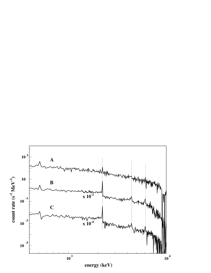
Figure 3: Background subtracted spectra of time intervals A, B and C. The dotted lines mark the nominal energies of the 2.223, 4.4 and 6.1 MeV lines.

In the spectrum of phase A, the 2.223 MeV line is very weak compared to phases B and C. The deexcitation lines can be hardly distinguished, while the continuum above 7 MeV seems comparatively stronger than in the two later phases. The line at 511 keV is also clearly visible but mainly of instrumental origin, and is therefore not considered in the present analysis. The same holds for the continuum below $\approx$600 keV, which is dominated by Compton scattered photons of higher energy and photons originating from pair creation reactions in the passive structural material. Spectra from phases B and C show a prominent narrow 2.223 MeV line, with a substantial Compton tail extending down to about 600 keV as well as clearly visible structures at 4.4 MeV and 6.1 MeV. They contain also the two ¹⁶O deexcitation lines around 7 MeV (Gros et al. [3]) as well as the lines from ²⁴Mg, ²⁰Ne and ²⁸Si. These lines are statistically significant but not obviously recognizable on the graphs.

3 Data analysis

The instrumental response to a monoenergetic gamma-ray flux in the present configuration, and especially in the several-MeV energy range is relatively complex and cannot be easily deduced from the ground calibration campaigns. A detailed description of the instruments and the calibration can be found in Vedrenne et al. [19] and Attié et al. [1]. The main differences to the standard response function are the strongly reduced full-energy peak efficiencies due to absorption and a continuum component from forward Compton scattered photons in the passive and active material of the satellite. Extensive Monte-Carlo simulations with the GEANT package and an approximate model of the spacecraft showed that essentially only the material close to the line Sun - Ge matrix is responsible for this component and in particular the matter sitting below the detector plane inside the BGO shield. These Compton scattered photons having lost only a small amount of energy contribute considerably to the continuum just below the line, which is of particular importance for the line shape calculations.

We made therefore Monte-Carlo simulations with the code MGGPOD (Weidenspointner et al. [21]) using the detailed SPI mass model (Sturner et al. [17]) coupled to the TIMM model (Ferguson et al. [2]) for the other parts of the spacecraft for gamma-ray energies corresponding to the lines observed at 1.37, 1.63, 1.78, 2.223, 4.4, 6.1 and 7 MeV. Monoenergetic beams of a projected area of 10098 cm² centered at the Ge-detector array with 10⁷ photons for each energy were generated in the simulations to obtain the spectral response for the lines of interest. The results for the full-energy peak effective detector areas and the transmission probabilities are listed in table 1. The transmission factors have been obtained assuming that the intrinsic efficiency of the detector array in this configuration equals the intrinsic efficiency of the Ge camera determined in the ground calibration campaign at Bruyères-le-châtel (Attié et al. [1]). Uncertainties of the effective area are estimated to be smaller than 10%. Uncertainties concerning the ratios of effective areas for different lines are estimated to be smaller than 5%.

Table 1: Effective areas and transmission factors of the SPI gamma-ray camera for the observation conditions of the flare obtained by MGGPOD simulations with a detailed model of SPI and the spacecraft.

Eγ (keV)	origin	eff. area (cm2)	transmission (%)
1369	24Mg${}^{\star}_{1369}$	3.6	2.8
1634	20Ne${}^{\star}_{1634}$	4.6	4.0
1779	28Si${}^{\star}_{1779}$	5.0	4.5
2223	1H(n,$\gamma$)2H	5.4	5.7
4438	12C${}^{\star}_{4439}$	5.2	8.7
6129	16O${}^{\star}_{6130}$	4.1	9.3
6916	16O${}^{\star}_{6917}$	3.6	9.4
7115	16O${}^{\star}_{7117}$	3.6	9.4

The spectra resulting from the simulations were then parameterized for the purpose of a global fit of the observed lines and the continuum during the different phases of the flare. The line components included a polynomial function describing the Compton tail at low energies from 600 keV up to the first escape peak. No attempts were made to describe the spectra below that energy region, for which the transmission gets anyway negligible. A second polynomial function was used to describe the Compton component between the first escape peak and the full-energy peak, multiplied by a function simulating the steplike behaviour of the Compton component below the full-energy peak. The first-escape and the full-energy peaks were taken as Gaussians. An example of the simulated spectrum for a gamma-ray line at 4438 keV with a FWHM of 88 keV and the described parameterization is shown in fig. 4.

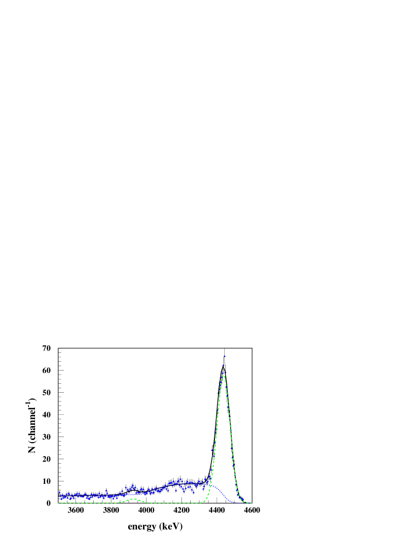
Figure 4: Symbols show the result of MGGPOD simulations for the response of SPI for an incident flux of gamma-rays with Gaussian energy distribution centered at 4438 keV and 88 keV FWHM for the particular observation conditions of the Oct. 28 flare. The different lines show the parameterization of the instrumental response function used for the global fits to the observed spectra. Dotted line: Compton component; dashed line: full-energy and first-escape peak; full line: sum of the components.

In a first analysis step, observed spectra of the different phases were fitted with the parameterized response of the three strongest lines at 2.223, 4.4 and 6.1 MeV, leaving the amplitudes, widths and line centroids (except for the fixed centroid of the 2223 keV line) as free parameters, and two components for the underlying continuum. The first component takes account of the bremssstrahlung continuum from accelerated electrons. A second continuum component between 600 keV and 2.223 MeV takes account of Compton scattering in the solar atmosphere of the 2.223 MeV gamma rays, because neutron capture on hydrogen may occur in depths reaching 10 g/cm². The photon flux incident on the satellite for this component was obained by simulating the transport of the 2.223 MeV gamma rays through the solar atmosphere with the GEANT package. We used several depth distributions of the neutron capture as shown in Hua & Lingenfelter [4] and choose finally an averaged photon spectrum approximating fairly well the different distributions.

This spectrum as well as the component from electron bremsstrahlung for which we choose an incoming power-law flux was then folded with the instrumental response function obtained from the GEANT and MGGPOD simulations as described above. We left the normalization factor for both continuum components as free parameters, limiting however the solar Compton scattering component to stay below the photon flux that was obtained from simulations using the deepest neutron capture depth distribution of Hua & Lingenfelter [4] (centered at about 10 g/cm²). This component, folded with instrumental response function could be fairly well described by a second order polynomial while the bremsstrahlung continuum could be described by a power-law function multiplied by an exponential above 2 MeV:

$$\frac{dN(E)}{dE}~{}\propto~{}E^{-s}~{}F_{exp}(E)$$ (1)

$F_{exp}(E)~{}=~{}1~{}~{}~{}~{}~{}~{}~{}~{}~{}~{}~{}~{}~{}~{}~{}~{}~{}~{}~{}~{}~{}~{}$ for E$<$2000 keV

$F_{exp}(E)~{}=~{}e^{-0.0003(E-2000)}~{}~{}$ for E$\geq$2000 keV

Fits were performed for spectra of the three phases between 600 keV and 8 MeV, excluding the energy bins 830-850, 1350-1370, 1610-1640, 1760-1780 keV and 6.8-7.2 MeV in phases B and C, where strong lines from ⁵⁶Fe, ²⁴Mg, ²⁰Ne, ²⁸Si and ¹⁶O deexcitation are situated. Fig. 5 shows the fit of the spectrum of the combined phases A, B and C, which include the main part of nuclear gamma-ray line emission of the flare. In the case of the phase A spectrum we fitted first the continuum part with the 2.223 MeV line complex, excluding the 4.4 and 6.1 MeV line ranges, and obtained then the parameters for the latter two lines by a fit to the residuals. All other spectra were fitted simultaneously with the continuum and the three lines. The spectra are fairly well fit throughout the whole region with these components. Results of the spectrum fits are presented in table 2.

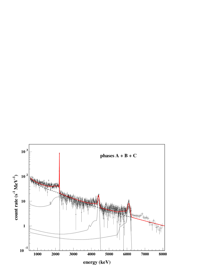
Figure 5: Background subtracted spectrum of time intervals A-C (symbols) with the result of the spectrum fit showing the sum of line and continuum components (full line). The line complexes including full-energy and first escape peak and the Compton tail are shown separately (dotted line). The excess around 7 MeV is due to the 6.9 and 7.1 MeV lines of ¹⁶O.The dashed line represents the continuum component.

Table 2: Results of the spectrum fits for the three strongest lines and the underlying continuum. Line centroids and $\sigma$ are in keV, rates are dead-time corrected counts/s and line fluences are expressed in photons/cm². S is the power-law index of the observed photon spectrum. Error bars result from the fit with an additional uncertainty of 10% for the fluences, due to an uncertainty on the effective area, added quadratically to the error bar of the fit.

	phase	A	B	C	A-C
continuum	s	0.87${}^{+0.02}_{-0.02}$	0.98${}^{+0.02}_{-0.02}$	1.11${}^{+0.03}_{-0.03}$	0.97${}^{+0.02}_{-0.02}$
(0.6-8 MeV)	rate	174${}^{+7}_{-2}$	142${}^{+3}_{-3}$	59${}^{+2}_{-2}$	95${}^{+2}_{-2}$
1H(n,$\gamma$)	rate	2.19${}^{+0.39}_{-0.42}$	15.2${}^{+0.5}_{-0.5}$	8.66${}^{+0.24}_{-0.24}$	9.65${}^{+0.21}_{-0.21}$
	fluence	30${}^{+6}_{-7}$	549${}^{+58}_{-58}$	721${}^{+75}_{-75}$	1286${}^{+132}_{-132}$
12C⋆	centroid	4400${}^{+10}_{-11}$	4398${}^{+5}_{-6}$	4415${}^{+6}_{-6}$	4407${}^{+4}_{-4}$
	$\sigma$	28${}^{+12}_{-6}$	40${}^{+8}_{-6}$	40${}^{+8}_{-6}$	37${}^{+5}_{-4}$
	rate	0.80${}^{+0.42}_{-0.35}$	1.86${}^{+0.28}_{-0.27}$	0.72${}^{+0.12}_{-0.12}$	1.01${}^{+0.12}_{-0.11}$
	fluence	12${}^{+6}_{-5}$	70${}^{+13}_{-12}$	62${}^{+12}_{-12}$	140${}^{+21}_{-21}$
16O⋆	centroid	-	6093${}^{+9}_{-8}$	6099${}^{+7}_{-6}$	6102${}^{+7}_{-7}$
	$\sigma$	-	59${}^{+10}_{-8}$	31${}^{+9}_{-7}$	57${}^{+8}_{-7}$
	rate	-	1.50${}^{+0.20}_{-0.20}$	0.35${}^{+0.08}_{-0.08}$	0.74${}^{+0.09}_{-0.09}$
	fluence	-	71${}^{+12}_{-12}$	38${}^{+9}_{-9}$	130${}^{+21}_{-21}$
$\chi^{2}_{d.o.f}$		1.06	1.25	1.08	1.24

With the exception of the ¹⁶O line in phase A statistically significant excess for the three studied gamma-ray lines could be observed during all phases. Line fluences for phases A-C comprise more than 95% of the total fluence for the two deexcitation lines and of about 90% for the neutron-capture line. With a total 2.223 MeV line fluence of about 1400 photons/cm², the October 28, 2003 flare is probably the one with the highest ever observed fluence for the neutron-capture line, exceeding the highest one observed by SMM on October 24, 1989 (Verstrand et al. [20]) by a factor of two and the one of the very intense June 4, 1991 solar flare observed by OSSE (Murphy et al. [9]) by about 40%.

There is a clear evolution of increasing spectral index s for the continuum from phases A to C and a rapidly increasing line-to-continuum ratio in the count rates between A and B, staying approximately stable afterwards. There is also evidence for a larger redshift of the ¹²C line - and to a lesser extent of the ¹⁶O line - during phase B compared to phase C and there is possibly a change in the 4.4 MeV to 6.1 MeV line flux ratio from phase B to C. We concentrate in the following on these two phases with strong nuclear line emission for a detailed line shape analysis.

4 Line shape analysis

We calculated the profile of the ¹²C line as described in Kiener et al. [6], where the 4.438 MeV gamma-ray production by accelerated protons and $\alpha$-particles interacting with ¹²C and ¹⁶O was based on extensive experimental data on total and differential cross sections and on measured line shapes. A similar approach was chosen for the 6.129 MeV gamma ray of ¹⁶O, produced by inelastic scattering off ¹⁶O and spallation of ²⁰Ne. The required nuclear reaction parameters were deduced from available cross section data, nuclear structure information and optical model calculations. We included also the 6.175 MeV line of ¹⁵O, produced mainly by spallation of ¹⁶O which could contribute to the high-energy tail of the 6.1 MeV line profile.

Due to uncertainties of the nuclear reaction models, the predicted line profiles F_calc(E) have to be taken with some caution. A comparison of calculated and measured line shapes in an accelerator experiment for the 4.4 MeV line at different angles with respect to incoming proton beam can be found in Kiener et al. [6]. We attribute therefore an uncertainty to the calculated line by assigning errors to the calculated profile $\Delta$F_calc(E) =  k  $\times$  F_calc(E) . A conservative estimate for k on the calculated line shape of the 4.4 MeV line is 0.2, whose calculations could be largely based on measured line shapes in the important energy range and 0.4 for the 6.1 MeV line, where no measured line shapes are available. Practically, we added these uncertainties quadratically to the error bars of the data for the line shape analyses.

All line shape calculations were based on a thick-target interaction model and were done with two different abundance sets of C, O and Ne. The first set are the chromospheric abundances of Reames [11]. These abundances are compatible with the observed fluence ratio between the carbon and the oxygen line $F_{4.4}/F_{6.1}$ in phase C; in a second set, we reduced the abundance of carbon by 50% with respect to oxygen, which fits better the line ratios of phase B and of the combined phases B-C. The same abundances relative to hydrogen were also used for the accelerated heavy ions producing broad lines by interacting with ambient hydrogen and helium nuclei with He/H = 0.1. These components are however typically a factor of five to ten smaller than the Compton component of the narrow lines in the energy region used for the fits. We therefore did not explore different accelerated heavy-ion to proton ratios. $\alpha$/p was left as a free parameter.

We added then to the calculated line profiles the Compton tails from the MGGPOD simulations and the continuum component from the global fit to the spectrum of the respective time interval. Comparison with the observed line profiles was done in the energy ranges 4280-4550 keV and 5955-6225 keV for the ¹²C and the ¹⁶O line, respectively. For the energy distribution of accelerated particles we used the same power-law spectrum in energy per nucleon for each species with an exponential cutoff at 200 MeV per nucleon. The spectral index s was deduced from the 2.223 MeV to the 4.4 and 6.1 MeV line fluence ratios to be in the range 3 $\leq$ s $\leq$ 4 (Tatischeff et al. [18]). Share et al.[15] find s $\approx$ 3 for the decay phase of the same flare . We made calculations with s = 3.0, 3.5 and 4.0. Three different particle angular distributions were used:

(1) A downward-directed (DW) distribution, where the angular distribution of energetic particles around the flare normal is given by:

$$\frac{dN}{d\Omega}~{}\propto~{}e^{-\Theta/\Delta\Theta}$$ (2)

with the flare normal taken to be perpendicular to the Sun’s surface and pointing towards the center of the Sun.

(2) A downward-isotropic (DI) distribution with:

$$\frac{dN}{d\Omega}~{}=~{}const.~{}~{}~{}\Theta\leq 90^{\circ}\newline \frac{dN}{d\Omega}~{}=~{}0~{}~{}~{}\Theta>90^{\circ}$$ (3)

(3) Pitch-angle scattering (PAS) distributions of Murphy et al. [8] with mean-free path parameters $\lambda$ = 30 and 300. They are based on a model of particle transport in coronal magnetic loops with constant field and converging field lines in the solar chromosphere and photosphere. Particles are injected isotropically into the loop and transported in the magnetic field taking account of pitch-angle scattering on MHD turbulence. $\lambda$ is defined in this model as the scattering mean free path divided by the half-length of the coronal segment of the magnetic loop. The angular distributions of the interacting particles producing gamma rays are governed by the competition between magnetic mirroring and pitch-angle scattering. Magnetic mirroring is dominant for $\lambda$ = 300 and the distribution approaches a fan beam parallel to the solar surface, while strong pitch-angle scattering $\lambda$ = 30 gives downward directed distributions. The different angular distributions are plotted in fig. 6.

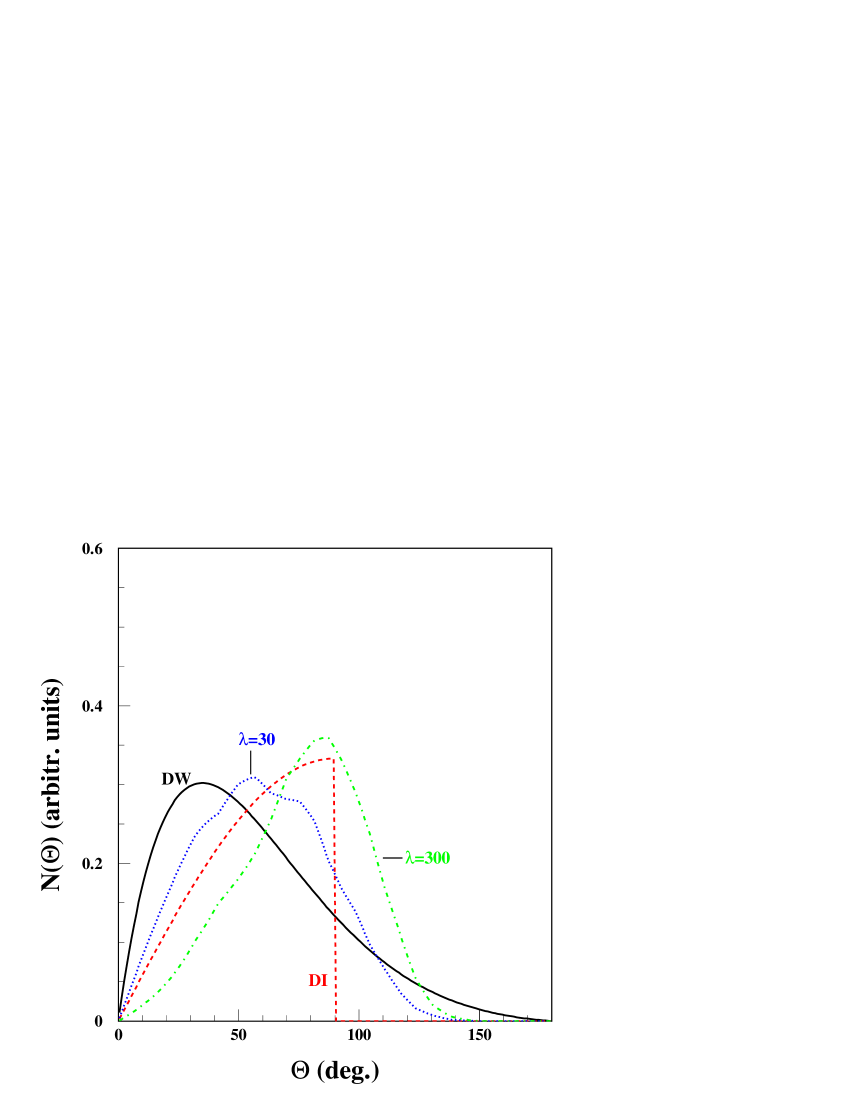
Figure 6: Relative number of interacting particles as a function of $\Theta$ used for the line shape calculations. $\Theta$ is the angle with respect to the flare axis, defined as the normal to the sun’s surface at the flare location. The DW distribution is for $\Delta\Theta$ = 40^∘

For the location of the flare, coordinates given by GOES for the start of the flare give a heliocentric angle $\Theta_{h}$ = 30^∘; RHESSI could resolve two emitting regions centered at $\Theta_{h}$ = 22^∘ and $\Theta_{h}$ = 25^∘ in the hard-X ray and 2.223 MeV gamma-ray line contours during the decline phase of the flare (Hurford et al. [5]). The exact position of the flare having practically no influence on the calculated line shapes we restricted calculations to one heliocentric angle. All following calculations were done with $\Theta_{h}$ = 25^∘ varying systematically $\alpha$/p and $\Delta\Theta$ in the case of DW distributions. A $\chi^{2}$ was obtained for each parameter set with a normalization factor for the calculated line shape adjusted to minimize $\chi^{2}$ with the MINUIT package of CERN. Estimated uncertainties of the theoretical line shapes as discussed above and of 10% for the Compton components were added quadratically to the error bars of the data.

We explored first the 4.4 and 6.1 MeV lines separately to get a new determination of the line fluences and test the validity of the results obtained with a Gaussian distribution. Best fits for the lines in time intervals B, C and the combined B-C and A-C intervals were mostly obtained with relatively narrow DW distributions of particles. However, DI and PAS(${\lambda=30}$) distributions in many cases gave also acceptable fits. Best-fit values of count rates and fluences are given in table 3. Count rates obtained with this method agree with the ones obtained by global fits of the spectra using Gaussian line shapes but are slightly more accurate despite the fact that the given error bars encompass all 1-sigma uncertainties of the different fits exploring a vast parameter space in spectral index, $\alpha$/p and particle-angular distributions. This analysis confirms that there is strong evidence for a change in the line fluence ratio, the ratio of count rates evolving from R_4.4/R_6.1 = 1.25${}^{+0.13}_{-0.13}$ in phase B to R_4.4/R_6.1 = 1.66${}^{+0.25}_{-0.25}$ in phase C.

Table 3: Results of separate fits to the ¹²C-line at 4.4 MeV and the ¹⁶O-line line at 6.1 MeV assuming a thick-target interaction model and three different energetic particle angular distributions around the flare axis. Rates and fluences are expressed as in table I. Error bars on count rates encompass the individual 1-sigma uncertainties of the different fits; a 10% uncertainty has been quadratically added to the error bars of line fluences.

	phase	B	C	B-C	A-C
12C⋆	$\alpha$/p	0.19	0.04	0.10	0.09
	$\Delta\Theta$	25∘	40∘	35∘	30∘
	rate	2.03${}^{+0.15}_{-0.17}$	0.68${}^{+0.09}_{-0.06}$	1.09${}^{+0.09}_{-0.07}$	1.02${}^{+0.10}_{-0.05}$
	fluence	76${}^{+9}_{-10}$	58${}^{+9}_{-8}$	127${}^{+16}_{-15}$	141${}^{+20}_{-16}$
16O⋆	$\alpha$/p	0.20	0.02	0.08	0.11
	$\Delta\Theta$	60∘	40∘	55∘	70∘
	rate	1.62${}^{+0.12}_{-0.09}$	0.40${}^{+0.06}_{-0.03}$	0.77${}^{+0.06}_{-0.04}$	0.74${}^{+0.06}_{-0.03}$
	fluence	77${}^{+10}_{-9}$	44${}^{+8}_{-6}$	121${}^{+15}_{-14}$	130${}^{+17}_{-14}$
24Mg⋆	fluence	45${}^{+15}_{-14}$	28${}^{+18}_{-18}$	75${}^{+24}_{-24}$	74${}^{+28}_{-24}$
20Ne⋆	fluence	34${}^{+13}_{-11}$	30${}^{+14}_{-13}$	63${}^{+24}_{-19}$	71${}^{+28}_{-20}$
28Si⋆	fluence	21${}^{+10}_{-9}$	20${}^{+11}_{-11}$	43${}^{+17}_{-14}$	50${}^{+19}_{-16}$

A similar approach was chosen to obtain the line fluences of the 1.37, 1.63 and 1.78 MeV gamma rays from ²⁴Mg, ²⁰Ne and ²⁸Si, respectively. We used the residual spectra for the fits. These spectra were obtained by subtracting the bremsstrahlung and solar Compton continuum and the Compton components of the three strongest lines at 2.223, 4.4 and 6.1 MeV obtained from the global fits (table 2). The energy regions around the respective lines were then fitted with a constant to take account of an eventual residual background and the calculated line shape which was folded with the instrumental response as in the case of the three strongest lines. For the line shape calculations we used available cross section data and proceeded otherwise as described in Ramaty et al. [10]. Line shapes of the three lines with best fit DW distributions are shown in fig.  7.

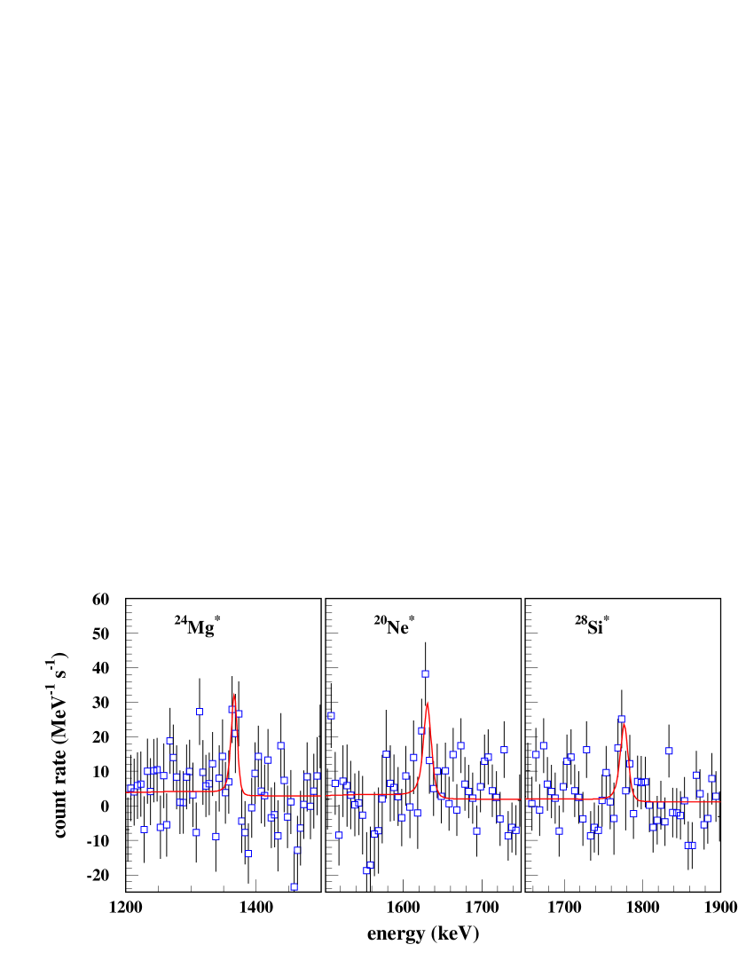
Figure 7: Calculated line shapes of the 1.37, 1.63 and 1.78 MeV lines for DW distributions with best fit parameters from combined fits to the 4.4 and 6.1 MeV lines. Data points represent the residual data of phases B-C after subtraction of the continuum components and the Compton tails of the lines at 2.223, 4.4 and 6.1 MeV.

Results for the count rates and line fluences are quoted in table 3. The uncertainties comprise all 1-sigma error bars from fits with three different energetic particle spectral indices, DW, DI and PAS angular distributions and with the best fit parameters $\alpha$/p and $\Delta\Theta$ that were obtained from combined fits to the 4.4 and 6.1 MeV lines as described below. Relative line fluences of the five lines are compatible with the ones observed by RHESSI for the July 23, 2002 flare (Smith et al. [16]) and with the exception of the ²⁰Ne line also compatible with the results from various flares observed by CGRO/OSSE and SMM (Murphy et al. [9]). It is interesting to note that the two satellites equipped with high-resolution Ge detectors give consistently a factor of about two smaller relative ²⁰Ne fluxes than the scintillation instruments.

Determinations of $\alpha$/p and the angular distributions were done by fitting simultaneously the 4.4 and 6.1 MeV lines. The same power-law energy spectra and the two different carbon abundances were used as in the case of individual fits to the lines. We like to stress that the line fluence ratio is not a free parameter in these fits but calculated with the thick-target interaction model used in the line shape calculations. This includes also the effect of the gamma-ray angular distribution with respect to the flare axis, which is different for 4.4 and 6.1 MeV gamma-ray emission, especially for very asymmetric energetic particle angular distributions as e.g. the narrow DW distributions. As expected for data of time intervals B, B-C and A-C, fits with the 50% reduced carbon-to-oxygen abundance ratio C/O gave systematically smaller $\chi^{2}$ than fits with nominal abundance, the difference being $\Delta\chi^{2}~{}\approx~{}$ 2-3. Surprisingly, combined fits of both lines had also slightly smaller $\chi^{2}$ ($\Delta\chi^{2}~{}\approx~{}$ 0.5-1.5) with reduced C/O for phase C, where the line fluence ratio does not necessarily favor a smaller carbon abundance. The following results were obtained with reduced C/O.

Table 4: Best fit values of angular distribution width parameter $\Delta\Theta$ for DW flares and of $\alpha$/p for DW and PAS($\lambda=30$) flares for combined fits of the ¹²C and ¹⁶O lines. Spectral index of accelerated particles s=4.0; values in parenthesis are for s=3.0. The values of $\alpha$/p and $\Delta\Theta$ for s=3.5 are generally between those of s=3.0 and s=4.0

flare geometry	DW			PAS
	$\alpha$/p	$\Delta\Theta$	$\chi^{2}$	$\alpha$/p	$\chi^{2}$
phase B	0.11 (0.19)	35∘ (30${}^{\circ})$	48.5 (48.8)	0.18 (0.35)	49.9 (52.1)
phase C	0.06 (0.00)	40∘ (40∘)	25.1 (26.8)	0.10 (0.03)	26.0 (27.2)
phase B-C	0.07 (0.11)	40∘ (35∘)	27.8 (28.7)	0.11 (0.19)	29.9 (31.3)

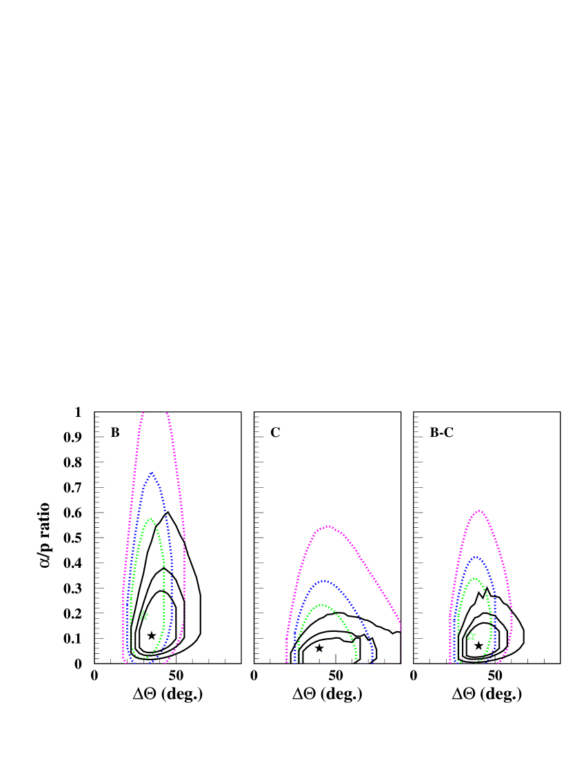
Figure 8: Contour lines in the $\alpha$/p - $\Delta\Theta$ parameter space of downward-directed particle distributions for simultaneous fits to the 4.4 and 6.1 MeV lines in flare phases B, C and B-C. Plotted are 50%, 70% and 90% confidence levels for fits using the reduced C/O and power-law particle spectra with s = 3.0 (dotted gray lines) and s = 4.0 (continuous black lines). $\chi^{2}$ minima are indicated by open (s = 3.0) and filled symbols (s = 4.0). The open symbol for phase C at $\alpha$/p = 0.00 $\Delta\Theta$ = 30^∘ is not plotted.

Best fits for all time intervals were obtained with a narrow DW distribution of the accelerated particles with $\Delta\Theta\approx$ 40^∘ and $\alpha$/p $\approx$ 0.1. The 50%, 70% and 90% confidence limit contours for these two parameters are shown in fig. 8. While the angular distribution of the energetic particles in phases B and C seems unchanged, an evolution of $\alpha$/p is possible with best fit values of 0.11 - 0.19 in phase B and a 90% upper limit of $\approx$ 1.1 to very low best fit values of 0.00 - 0.06 in phase C, with a 90% upper limit at $\approx$ 0.6. These lower $\alpha$/p fit values result from smaller redshifts of the 4.4 and 6.1 MeV line and a smaller width of the 6.1 MeV line in phase C. These facts could also be explained by differences in flare geometry or an evolution of the power-law index, however, a change in $\alpha$/p would explain also naturally the different line ratios. For example, reducing $\alpha$/p from 0.2 to 0.00 increases the C/O line ratio by 25%, which is consistent with the line-ratio evolution between phase B and C. This can hardly be achieved by varying power-law index or flare geometry, and the only other explanation would be a surprising abundance change of C or O in the interaction region.

We investigated also the line shapes resulting from DI and PAS distributions. With the pitch-angle scattering distributions of the model of Murphy et al. (1990), the distribution with $\lambda$ = 300 could be excluded at the 99.7% level in phases B, B-C and A-C and at the 95.4% level in phase C. Fits with $\lambda$ = 30 described the lines not as good as the best fit DW distributions but stayed generally inside the 1-sigma confidence level with slightly higher $\alpha$/p. DI distributions gave similar $\chi^{2}$ values and $\alpha$/p as PAS(${\lambda=30}$) ones. Examples of calculated line shapes representing best fit DW distributions are presented in fig. 10; line shapes for best fit PAS and DI distributions are shown in fig. 9. One can see in fig. 10 that observed line shapes in the fit region depend practically only on the narrow component, the broad component from accelerated heavy-ion interactions being even significantly smaller than the Compton tail.

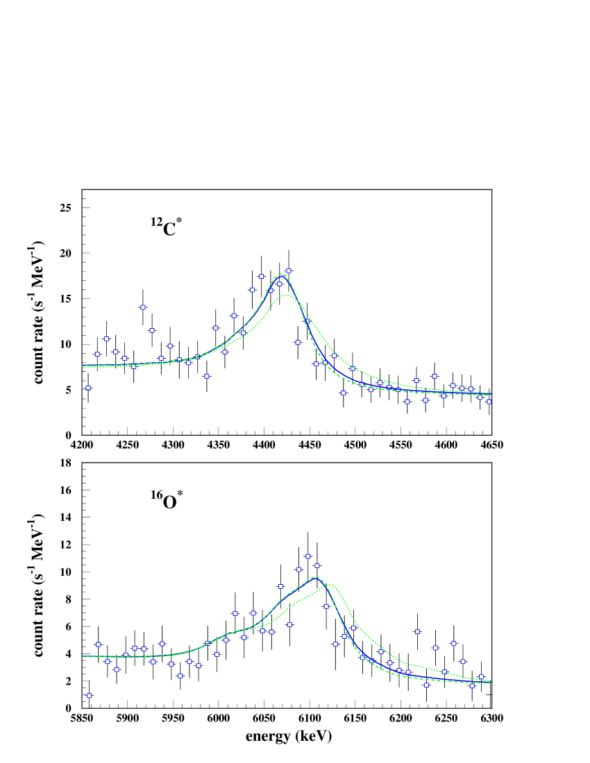
Figure 9: Calculated line shapes for best fit parameters of DI (dashed line), PAS($\lambda=30$) (full line) and PAS($\lambda=300$) (dotted line) energetic particle distributions in comparison with observational data of time interval B-C. The line shapes of PAS($\lambda=30$) and DI distributions are practically indistinguishable.

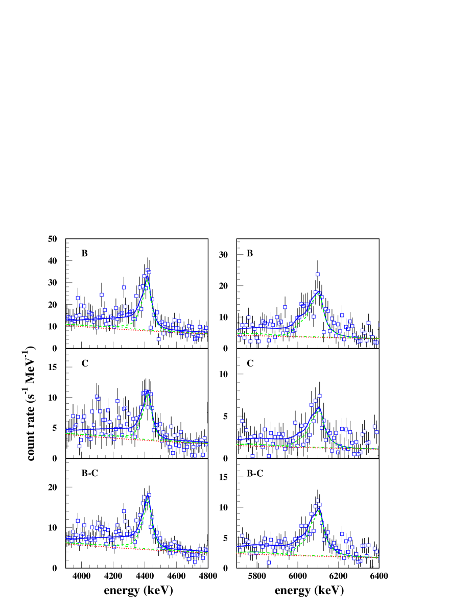
Figure 10: Calculated line shapes of the ¹²C line at 4.4 MeV (left) and the ¹⁶O line at 6.1 MeV (right) for best fit parameters of downward-directed flares in comparison with observational data for time intervals B, C and B-C. Dotted line: continuum component, dashed-dotted line: continuum plus broad line component, dashed line: continuum plus narrow and broad line component, full line: sum of line, continuum and Compton component.

All line shapes are quite nicely reproduced by the calculated ones, the reduced $\chi^{2}$ values being about 0.5 for phases C and B-C and about 1.0 for phase B, except for PAS($\lambda=300$) distributions which provide bad fits to the data. Such low $\chi^{2}$ values can be explained by our estimated uncertainties of theoretical shapes which were added to the error bars of the data. The theoretical uncertainty is particularly important for the 6.1 MeV line, in fact comparable with its statistical uncertainty. This illustrates that still better constraints could be obtained from observations with the new generation gamma-ray satellites by improved knowledge of some important nuclear reactions leading to strong gamma-ray emission in solar flares.

5 Conclusion

The very intense gamma-ray flare of October 28, 2003 was observed by the gamma-ray spectrometer SPI onboard INTEGRAL in the energy range from 600 keV to 8 MeV and by the Anti-Coincidence Shield of SPI above 150 keV. Time profiles show three different phases of gamma-ray emission. In the first minute, an emission peak was observed consisting mainly of continuum emission from electron bremsstrahlung with very little nuclear line emission. In a second phase which lasted $\approx$3.5 minutes, high flux levels containing several peaks with strong nuclear line and continuum emission could be observed, before a smooth decay phase of a about ten minutes of both emission components terminates the gamma-ray flare.

A power-law bremsstrahlung component and three prominent narrow nuclear lines at 2.223 MeV from neutron capture on hydrogen, at 4.4 MeV from ¹²C deexcitation and at 6.1 MeV line from ¹⁶O deexcitation were observed during the three phases. There is clear evidence of a change in continuum power-law index and the continuum-to-line ratio during the flare. More surprisingly, the flux ratio of the 4.4 MeV to 6.1 MeV lines shows a significant change between the second and third phase of the flare. This line ratio evolution could be confirmed by detailed line shape analyses of both nuclear deexcitation lines based on thick-target interaction model of the accelerated particles with the solar atmosphere and a set of recent nuclear data and reaction calculations. The overall line ratio, in particular the line ratio of the second phase, points to a significantly reduced carbon abundance with respect to oxygen in the composition of the target solar atmosphere.

Best fits of both lines resulting from a systematic scan of $\alpha$/p and the width of the particle angular distribution indicated equally an evolution between the second and third flare phase. While both phases clearly favor a narrow downward-directed particle beam perpendicular to the solar surface, $\alpha$/p could have been higher in the second than in the third phase. Such a drop of the energetic $\alpha$-particle content would also naturally explain the observed change in the 4.4 MeV to 6.1 MeV line ratio between both phases. We conclude that the simplest and most probable explanation is an evolution of $\alpha$/p during the second and third phase of the flare.

The observation of solar flares with high-resolution gamma-ray spectrometers, like the ones of RHESSI and INTEGRAL, both launched in 2002 opened up new possibilities of detailed line shape analyses to constrain properties of the accelerated particle distributions. In this paper, we could obtain tight constraints on the particle angular distributions and interesting evidence for temporal evolution of the alpha-to-proton ratio. These studies will now be applied to other recently observed flares.

6 Acknowledgements

Based on observations with INTEGRAL, an ESA project with instruments and science data centre funded by ESA member states (especially the PI countries: Denmark, France, Germany, Italy, Switzerland, Spain), Czech Republic and Poland, and with the participation of Russia and the USA. We thank A. Bykov, P.I. of the INTEGRAL observation during the flare, who gave us rapid access to the data.

References

- [1] Attié, D., Cordier B., Gros, M., et al. 2003, Astronomy and Astrophysics 411, L71
- [2] Ferguson C., Barlow, E.J., Bird, A.J., et al. 2003, Astronomy and Astrophysics 411, L19
- [3] Gros, M., Tatischeff, V., Kiener, et al 2004, in Proc. 5th INTEGRAL Workshop, the INTEGRAL Universe, Munich, Germany, 16-20 February 2004, ed. V. Schönfelder, G. Lichti & C. Winkler, ESA SP-552, 669
- [4] Hua, X.-M., & Lingenfelter, R.E. 1987, Solar Physics 107, 351
- [5] Hurford, G.J., Krucker, S., Lin, R.P., Schwartz, R.A., Share, G.H., & Smith, D.M. 2005, Astrophysical Journal Letters, in preparation
- [6] Kiener, J., de Séréville, N., & Tatischeff, V. 2001, Physical Review C 64, 025803
- [7] Murphy, R.J., Kozlovsky, B., & Ramaty, R. 1988, Astrophysical Journal 331, 1029
- [8] Murphy, R.J., Hua, X.-M., Kozlovsky, B., & Ramaty, R. 1990, Astrophysical Journal 351, 299
- [9] Murphy, R.J., Share, G.H., Grove, J.E., Johnson, W.N., Kinzer R.L., Kurfess, J.D., Strickman, M.S., & Jung G.V. 1997 Astrophysical Journal 490, 883
- [10] Ramaty, R., Kozlovsky, B., & Lingenfelter, R.E. 1979, Astrophysical Journal Suppl. Ser., 40, 487
- [11] Reames, D.V 1999, Space. Sci. Rev., 90, 413
- [12] Share, G.H., & Murphy, R.J. 1997, Astrophysical Journal 485, 409
- [13] Share, G.H., Murphy, R.J., Kiener, J., & de Séréville, N. 2002, Astrophysical Journal 573, 464
- [14] Share, G.H., Murphy, R.J., Skibo, J.G., Smith, D.M., Hudson, H.S., Lin, R.P., Shih, A.Y., Dennis, B.D., Schwartz, R.A., & Kozlovsky, B. 2003, Astrophysical Journal 595, L85
- [15] Share, G.H., Murphy, R.J., Smith, D.M., Schwartz, R.A., & Lin, R.P. 2004, Astrophysical Journal 615, L169
- [16] Smith, D.M., Share, G.H., Murphy, R.J., Schwartz, R.A., Shih, A.Y., & Lin, R.P. 2003, Astrophysical Journal 595, L81
- [17] Sturner, S.J., Shrader, C.R., Weidenspointner, G., Teegarden B.J., et al. 2003, Astronomy and Astrophysics 411, L81
- [18] Tatischeff, V., Kiener, J., & Gros, M. 2004, in Proceedings 5th Rencontres du Vietnam, New Views on the Universe, Hanoi, Vietnam
- [19] Vedrenne, G., Roques, J.-P., Schönfelder, V., Mandrou, P., et al.: 2003 Attié, D., Cordier B., Gros, M., Laurent, Ph., et al. 2003, Astronomy and Astrophysics, 411, L63
- [20] Verstrand W.T., Share G.H., Murphy, R.J., Forrest D.J., Chupp, E.L., & Kanbach, G. 1999, Astrophysical Journal Suppl. Ser., 120, 409
- [21] Weidenspointner, G., Harris, M. J., Sturner, S., Teegarden, B.J., & Ferguson C. 2005, Astrophysical Journal Suppl. Ser. 156, 69
- [22] Weidenspointner, G., Kiener, J., Gros, M., et al. 2003, Astronomy and Astrophysics, 411, L113
- [23] Werntz, C., Lang, F.L., & Kim, Y.E. 1990, Astrophysical Journal Suppl. Ser. 73, 349