Cosmic Shear Analysis with CFHTLS Deep data

We present the first cosmic shear measurements obtained from the T0001 release of the Canada-France-Hawaii Telescope Legacy Survey. The data set covers three uncorrelated patches (D1, D3 and D4) of one square degree each, observed in $u^{*}$, $g^{\prime}$, $r^{\prime}$, $i^{\prime}$ and $z^{\prime}$ bands, to a depth of $i^{\prime}=25.5$. The deep, multi-colour observations in these fields allow for several data-quality controls. The lensing signal is detected in both $r^{\prime}$ and $i^{\prime}$ bands and shows similar amplitude and slope in both filters. $B$-modes are found to be statistically zero at all scales. Using multi-colour information, we derived a photometric redshift for each galaxy and use this to separate the background source sample into low-z and high-z subsamples. A stronger shear signal is detected from the high-z subsample than from the low-z subsample, as expected from weak lensing tomography. While further work is needed to model the effects of errors in the photometric redshifts, this result suggests that it will be possible to obtain constraints on the growth of dark matter fluctuations with lensing wide field surveys. The combined Deep and Wide surveys give $\sigma_{8}=0.89\pm 0.06$ assuming the Peacock & Dodds non-linear scheme (P&D), and $\sigma_{8}=0.86\pm 0.05$ for the halo model and $\Omega_{m}=0.3$. We assumed a Cold Dark Matter model with flat geometry and have marginalized over the systematics, the Hubble constant and redshift uncertainties. Using data from the Deep survey, the $1\sigma$ upper bound for $w_{0}$, the constant equation of state parameter is $w_{0}<-0.8$.

1 Introduction

Cosmological weak lensing, also called cosmic shear, can be used to probe the dark matter distribution in the universe. Weak lensing observations complement other probes such as CMB anisotropies (Spergel et al. (2003)), type Ia supernovae (Riess et al. (2004, 1998); Perlmutter et al. (1999)), and redshift surveys (Lahav & Suto (2004)). Weak lensing also has the advantage of being free of any assumption regarding the light versus matter distributions (Mellier (1999); Bartelmann & Schneider (2001); Van Waerbeke & Mellier (2003); Réfrégier (2003)).

It has only recently been shown that cosmic shear measurement is technically feasible (Bacon, Réfrégier & Ellis (2000); Kaiser et al. (2000); Van Waerbeke et al. (2000); Wittman et al. (2000)). Unfortunately, the deepest weak lensing survey has a sky coverage limited to less than one deg² and the widest to $\sim$10 deg². Moreover, most surveys were performed in one colour only, and even rough redshift information was not available. These limitations restricted the use of weak lensing as a cosmological probe to a very small number of parameters. Early weak lensing surveys were primarily focused on the measurements of the normalization of the dark matter power spectrum, $\sigma_{8}$, and the mass density parameter, $\Omega_{m}$. The most recent cosmic shear surveys reach a relative accuracy of about 10% on $\Omega_{m}\,\sigma_{8}^{0.5}$ (Mellier (1999); Bartelmann & Schneider (2001); Van Waerbeke & Mellier (2003); Réfrégier (2003)), but the uncertainty on other parameters is still fairly large.

Second generation cosmic shear surveys are now under way and will provide the community with multi-colour data of excellent image quality, over a wide field of view. The Canada-France-Hawaii Telescope Legacy Survey (CFHTLS), using the recently built MegaPrime/Megacam wide field camera, belongs to this generation. The CFHTLS-Wide survey (the core of the CFHTLS cosmic shear survey) will provide a large sky coverage of 170 deg.², and the deep four deg.² CFHTLS-Deep will provide shear information on smaller scales and as a function of lookback time, out to higher redshift than the CFHTLS-Wide .

Both surveys will ultimately consist of complete and homogeneous panchromatic data in $u^{*}$,$g^{\prime}$,$r^{\prime}$,$i^{\prime}$,$z^{\prime}$. The data were taken between June 1st 2003 and July 22, 2004 as part of a preliminary survey to provide detailed quality assessments and propose technical or operational improvements, when necessary. The CFHTLS-Wide has the same depth as Virmos-Descart, but so far, the available data is only in one colour and covers $\approx 20$ deg². A cosmic shear analysis with the wide data is performed in Hoekstra et al. (2005). The CFHTLS-Deep has been observed in all five filters, therefore photometric redshift are available, and will be used in this work. Moreover, the CFHTLS D1 Deep field is located in the Virmos-VLT Deep Survey (VVDS) F02 field which has several thousand of galaxy redshifts (Le Fèvre et al. (2005)) and near infrared data (on a tiny area). A combination of large and small scales from the Wide and the Deep data will ultimately provide an excellent data set to probe the nature of dark energy in the universe (Cooray & Huterer (1999); Benabed & Bernardeau (2001); Linder & Jenkins (2003); Benabed & van Waerbeke (2004); Jarvis et al. (2005)). In this work, we describe the first CFHTLS cosmic shear studies based on Deep data, and then combine the Wide and Deep data analysis to derive constraints on $\Omega_{m}$ and $\sigma_{8}$.

The organization of the paper is as follows. In section 2 we introduce the notation and define the statistics we use. The data set is described in Section 3. In section 4 and 5 we present results and residual systematics and we discuss them. Conclusions and perspectives are outlined in Section 6.

2 Theoretical background

The theory of weak lensing has been previously been discussed in detail in the literature, including the physical motivations of various approximations (e.g. Bartelmann & Schneider (2001)). Following Hoekstra (2004); Van Waerbeke et al. (2002); Van Waerbeke, Mellier & Hoekstra (2005) we follow the notation of Schneider et al. (1998).

We introduce the power spectrum of the convergence $\kappa$ as :

$$P_{\kappa}(k) = {9\over 4}\Omega_{0}^{2}\int_{0}^{\chi_{H}}{{\rm d}\chi\over a^{2}(\chi)}P_{3D}\left({k\over f_{K}(\chi)};\chi\right)\times$$ (1)

$$\left[\int_{\chi}^{\chi_{H}}{\rm d}\chi^{\prime}n(\chi^{\prime}){f_{K}(\chi^{\prime}-\chi)\over f_{K}(\chi^{\prime})}\right]^{2},$$

were $f_{K}(\chi)$ is the comoving angular diameter distance out to radial distance $\chi(z)$, and $n(\chi)$ is the redshift distribution of the sources. $P_{3D}\left({k\over f_{K}(\chi)},\chi\right)$ is the 3-dimensional mass power spectrum, and $\kappa$ is a 2-dimensional wave vector perpendicular to the line-of-sight.

Cosmic shear can be studied using three different 2-point statistics, which differ only by their filtering schemes. These various statistics have different wavelength sensitivities to the power spectrum and therefore the effect of systematics on each is different. This enables the comparison of multiple cross-checked solutions. Two-point statistics are measured as a function of scale $\theta_{c}$, which could either be a galaxy pair separation or smoothing window radius. The relation between each two-point statistics and the power spectrum of the gravitational convergence (i.e. the projected dark matter power spectrum) can be expressed as follows:

• Top-hat variance:

  $$\langle\gamma^{2}\rangle_{\theta_{c}}={2\over\pi\theta_{c}^{2}}\int_{0}^{\infty}\leavevmode\nobreak\ {{\rm d}k\over k}P_{\kappa}(k)[J_{1}(k\theta_{c})]^{2}.$$ (2)

• Shear correlation function:

  $$\langle\xi\rangle_{\theta_{c}}={1\over 2\pi}\int_{0}^{\infty}\leavevmode\nobreak\ {\rm d}k\leavevmode\nobreak\ kP_{\kappa}(k)J_{0}(k\theta_{c}).$$ (3)

• Aperture mass variance:

  $$\langle M_{\rm ap}^{2}\rangle_{\theta_{c}}={288\over\pi\theta_{c}^{4}}\int_{0}^{\infty}\leavevmode\nobreak\ {{\rm d}k\over k^{3}}P_{\kappa}(k)[J_{4}(k\theta_{c})]^{2},$$ (4)

with the aperture mass variance defined as:

$$M_{\rm ap}(\theta_{c})=\int_{\theta<\theta_{c}}\leavevmode\nobreak\ {\rm d}^{2}{{\hbox{$\bf\theta$}}}\ \kappa({{\hbox{$\bf\theta$}}})\leavevmode\nobreak\ U(\theta),$$ (5)

where $U(\theta)$ is a compensated filter such as:

$$U(\theta)={9\over\pi\theta_{c}^{2}}\left(1-{\theta^{2}\over\theta_{c}^{2}}\right)\left({1\over 3}-{\theta^{2}\over\theta_{c}^{2}}\right).$$ (6)

$M_{\rm ap}$ can be expressed in terms of the tangential shear component inside a circle as follows (Kaiser et al. (1994); Schneider (1996)) :

$$M_{\rm ap}(\theta_{c})=\int_{\theta<\theta_{c}}\leavevmode\nobreak\ {\rm d}^{2}{{\hbox{$\bf\theta$}}}\ \gamma_{t}({{\hbox{$\bf\theta$}}})\leavevmode\nobreak\ Q(\theta),$$ (7)

where the tangential shear component $\gamma_{t}({{\hbox{$\bf\theta$}}})$ at the position $\bf\theta$ is given by:

$$\gamma_{t}({{\hbox{$\bf\theta$}}})=-{\mathcal{R}e}\,\left(\gamma\left({{\hbox{$\bf\theta$}}}\right)\right)e^{-2i\phi}$$ (8)

and the function $Q(\theta)$ is defined as :

$$Q(\theta)=\frac{2}{\theta^{2}}\int^{\theta}_{0}d\theta^{\prime}\leavevmode\nobreak\ \theta^{\prime}\leavevmode\nobreak\ U(\theta^{\prime})-U(\theta)\,.$$ (9)

The aperture mass statistic as a tool for the cosmic shear analysis has been discussed in many papers (Schneider et al. (1998); Pen, van Waerbeke & Mellier (2002); Munshi & Coles (2003); Munshi & Valageas (2005)). This statistic is sensitive to curl-free correlations (E-modes) generated by the (scalar) gravitational potential. Curl correlations (B-modes) are then easily derived using the same statistics, after rotating each galaxy by $45\,deg$. If the only signal present is due to lensing, then the B-modes should be zero at all scales. This simple procedure is therefore a powerful diagnostic tool to assess systematic residuals in cosmic shear signal.

Unfortunately, the $M_{ap}$ statistic is sensitive to the smallest accessible angular scales, where cosmic shear signal depends on the poorly-known non-linear evolution of the dark matter power spectrum. This shortcoming forces us to compute E- and B-modes on larger angular scales in a different way. For this we use the top-hat shear variance and the shear correlation functions. These functions are usually derived from the $\xi_{+}$ and $\xi_{-}$ shear correlation functions:

$$\xi_{+}(r) = \langle\gamma_{t}(\theta)\gamma_{t}(\theta+r)\rangle+\langle\gamma_{r}(\theta)\gamma_{r}(\theta+r)\rangle.$$

$$\xi_{-}(r) = \langle\gamma_{t}(\theta)\gamma_{t}(\theta+r)\rangle-\langle\gamma_{r}(\theta)\gamma_{r}(\theta+r)\rangle,$$ (10)

where $\gamma_{t}$ and $\gamma_{r}$ are the tangential and radial projections of the shear onto the local frame joining two galaxies separated by a distance $r$. Following Crittenden et al. 2001a , we define

$$\xi^{\prime}(r)=\xi_{-}(r)+4\int_{r}^{\infty}\frac{dr^{\prime}}{r^{\prime}}\xi_{-}(r^{\prime})-12r^{2}\int_{r}^{\infty}\frac{dr^{\prime}}{r^{\prime 3}}\xi_{-}(r^{\prime}).$$ (11)

The $E$ and $B$ shear correlation functions are given by

$$\xi^{E}(r)=\frac{\xi_{+}(r)+\xi^{\prime}(r)}{2}\ \ \ \ \ \ \xi^{B}(r)=\frac{\xi_{+}(r)-\xi^{\prime}(r)}{2}.$$ (12)

A similar relation can be found for the aperture mass and the top-hat statistics as showed in Crittenden et al. 2001b . Crittenden et al. 2001b also pointed out $\xi^{E}$ and $\xi^{B}$ can only be derived up to an integration constant which depends on the extrapolated signal outside the measurement range.

Finally, the amplitude of the lensing signal depends on the galaxy redshift distribution $n(z)$ (see Eq.(1)). As in previous works (see Van Waerbeke et al. (2002); Van Waerbeke, Mellier & Hoekstra (2005)), we use the following redshift distribution:

$$n(z)=\frac{\beta}{z_{s}\;\Gamma\Big{(}\frac{1+\alpha}{\beta}\Big{)}}\Big{(}\frac{z}{z_{s}}\Big{)}^{\alpha}\;\exp\,\Big{[}{-\Big{(}\frac{z}{z_{s}}\Big{)}^{\beta}}\Big{]}\ ,$$ (13)

where $\alpha$, $\beta$ and $z_{s}$ parameters are derived from deep photometric redshift catalogues. The lensing signal can be predicted for any redshift range using Eq.(1) and Eq.(13).

3 The Deep CFHTLS T0001 data set

The Deep CFHTLS data used in this work consists of $u^{*}$, $g^{\prime}$, $r^{\prime}$, $i^{\prime}$ and $z^{\prime}$ stacked Megacam images that form the first CFHTLS release (hereafter T0001). The release is composed of stacked images, catalogues and relevant meta-data produced from observations in four uncorrelated fields that were carried out at CFHT with the Megaprime instrument between June 1st 2003 and July 22, 2004. Details regarding each field are listed on the CFHTLS web pages.

Each Megacam image consists of an array of 9 $\times$ 4 EEV CCDs of 2048 $\times$ 4612 pixels each (Boulade et al. (2003)). The pixel scale is 0.186” and the camera covers a total field of 1 degree $\times$ 1 degree. There are two large gaps of 82 arc-second between rows of CCDs. In order to produce complete fields, the gaps have been filled by organizing observations in a series of exposure sequences with large offsets. This results in an heterogeneous pixel illumination at the borders of each CCD. This spatial flux variation induces a varying pixel signal-to-noise ratio that is taken into account by using pixel weight maps together with hand-made masks (see Section 4) to discard noisy areas of each field.

The stacks include only Megacam images with seeing better than 1.0” and airmass below 1.4 have been selected. However, because there were fewer $u^{*}$-band images than for the other filters, we relaxed the selection criteria for this filter and kept all $u^{*}$ images with seeing below 1.4”. Only three of the four Deep fields have been selected for cosmic shear studies. The D2 Deep field has been dropped from our sample because it is significantly shallower than the other three fields.

Data were calibrated and processed at CFHT and the Terapix data center. The full T0001 release is archived at CADC and available to any CFHTLS registered user. A description of the data processing pipeline used to produce the deep T0001 stacks is beyond the scope of the paper, but the details can be found on the Terapix web pages. Photometric and astrometric methods and quality assessments done on these data are explained in a short explanatory supplement. The processing (astrometric and photometric calibrations, pixel re sampling, image warping and stacking, catalogue production) uses the current first generation Terapix software tools and closely follows the one used for the Virmos-Descart survey that is described in McCracken et al. (2003). We refer to this paper, and to the Terapix and CFHT web pages for further details.

The accuracy of the photometric calibrations can be estimated from the stellar colour-colour plots and the galaxy counts in all bands given on the Terapix T0001 pages and is also discussed in the more detailed stellar analysis done by Schulteiss et al. (in preparation). In all bands, the cumulative internal and systematic photometric errors are 0.05 mag up to AB=22.5, and never larger than 0.1 to the 80% completeness limit ($\approx$ AB=25.5). This uncertainty is sufficient for the cosmic shear studies on this paper.

Table 1: Summary table of T0001 D1, D3 and D4 deep stacks used in this work. Magnitudes are instrumental AB. Details on magnitude, aperture, seeing and completeness definitions are given in the explanatory page http://terapix.iap.fr/article.php?id_article=383

	D1	D3	D4
RA (J2000)	02:25:59	14:19:27	22:15:31
DEC (J2000)	-04:29:40	+52:40:56	-17:43:56
Effective FOV (deg2)	0.80	0.77	0.77
Exp. time $u^{*}$ (s)	10560	4620	16680
Median seeing $u^{*}$ (arc-sec.)	1.15	0.88	1.05
Completeness $u^{*}$ 50% (mag.)	26.4	26.0	26.2
Exp. time $g^{\prime}$	7515	8010	11250
Median seeing $g^{\prime}$ (arc-sec.)	0.98	0.95	0.99
Completeness $g^{\prime}$ 50% (mag.)	26.4	26.5	26.2
Exp. time $r^{\prime}$	17280	20820	26400
Median seeing $r^{\prime}$ (arc-sec.)	0.87	0.93	0.85
Completeness $r^{\prime}$ 50% (mag.)	26.1	26.4	25.9
Exp. time $i^{\prime}$	52000	59640	58800
Median seeing $i^{\prime}$ (arc-sec.)	0.88	0.92	0.88
Completeness $i^{\prime}$ 50% (mag.)	26.1	26.2	25.8
Exp. time $z^{\prime}$	12240	15120	-
Median seeing $z^{\prime}$ (arc-sec.)	0.86	0.85	-
Completeness $z^{\prime}$ 50% (mag.)	24.5	24.6	-

Table 1 summarizes the T0001 stacks used in this work. The completeness limits have been computed by adding randomly simulated stars (Moffat profiles) inside a 2000$\times$2000 area of each Deep field and by running the detection and photometry again, using the MAG_AUTO magnitude of SExtractor software (Bertin & Arnouts (1996)). The completeness was also checked using galaxy counts .

The D4-$z^{\prime}$ data have not been released by Terapix because the astrometric internal accuracy was below the scientific requirements. The large rms error found in the D4-$z^{\prime}$ data is not been fully understood, but it results in a large number of galaxy mismatches during the $u^{*},g^{\prime},r^{\prime},i^{\prime},z^{\prime}$ catalogue cross-identification. This hampers reliable panchromatic studies for many galaxies detected in this field. A further investigation reveals that the D4$-i^{\prime}$ astrometric solution is also slightly off, while data quality in other filters are excellent. Although it has no impact on the D4-$u^{*},g^{\prime},r^{\prime},i^{\prime}$ photometric studies, a quick weak lensing analysis of the D4-$i^{\prime}$ field shows it has more systematic residuals than D1-$i^{\prime}$ and D3-$i^{\prime}$. In contrast, the three Deep $r^{\prime}$ band data have similar quality and do not show systematics residual differences. We therefore used the $r^{\prime}$ band as the reference data set for all comparison between the fields, and only use the deep D1/D3 $i^{\prime}$ band data for colour comparisons, when needed.

4 Detection of the shear signal

4.1 Galaxy shape parameters

Catalogues and shape measurements of galaxies are produced using the IMCAT software (Kaiser et al. (1995), hereafter KSB). For each object the centroid position and the half-light radius $r_{h}$ are measured. These parameters are then used to derive orientations and raw ellipticities of galaxies from the weighted second moments $I_{ij}$ of the galaxy light distribution. In order to minimize the noise contribution each moment is filtered using a Gaussian filter $W(\theta)$ of size $r_{h}$:

$$I_{ij}=\int d^{2}\mathbf{\theta}\,W\left(\theta\right)\ \theta_{i}\,\theta_{j}\,(\mathbf{\theta})\ f(\mathbf{\theta})\;,$$ (14)

where $f(\mathbf{\theta})$ is the surface brightness.

The raw ellipticity is given by:

$$\mathbf{e}=\left(\frac{I_{11}-I_{22}}{{\mathcal{T}r\left(I\right)}};\;\frac{2\,I_{12}}{{\mathcal{T}r\left(I\right)}}\right)\;.$$ (15)

where $\mathcal{T}r(I)$ represents the trace of the matrix $I$. We use the KSB method to get an unbiased estimator of the shear $\mathbf{\gamma}$. This method has been tested by several teams and it has been demonstrated that it provides robust and reliable shear measurements from ground based data (see the comprehensive critical investigation of KSB and other techniques by Heymans et al. 2005b , and also references therein).

4.1.1 PSF correction: the principle

Let us assume the shear-free intrinsic ellipticity of a galaxy is $\mathbf{e}^{0}$. On the detector, its shape is eventually modified by the distortions produced by gravitational lensing effects and systematics that increase the smearing and the anisotropic component of the PSF (atmosphere, optical aberrations). Assuming these distortions are small, Kaiser et al. (1995) demonstrated the observed ellipticity, $\mathbf{e}^{obs}$, can be written:

$$\mathbf{e}^{obs}_{\alpha}=\mathbf{e}^{0}_{\alpha}+P^{sh}_{\alpha\beta}\mathbf{\gamma}+P^{sm}_{\alpha\beta}\mathbf{q}\ ,$$ (16)

where $\mathbf{q}$ is the anisotropic component of the PSF and $\mathbf{\gamma}$ is the gravitational shear.  $P^{sh}$ and $P^{sm}$ are called the shear and the smear polarisability. Their values depend on the galaxy surface brightness and on the filter properties $W(\theta)$.  $\mathbf{q}$ can be derived directly from the data, by measuring the ellipticity of stars in each field, $\mathbf{e}_{\star}$, such as:

$$\mathbf{q}_{\alpha}=\frac{\mathbf{e^{\star}}_{\alpha}}{P^{sm}_{\beta\beta}}\;.$$ (17)

The shear polarisability is however altered by the isotropic smearing component of the PSF. It results in a modification of the shear polarisability

$$P^{\gamma}=P^{sh}-\frac{P^{sh}_{\star}}{P^{sm}_{\star}}P^{sm}\;,$$ (18)

where $P^{\gamma}$ is called pre-seeing shear polarisability and $P^{sh/sm}_{\star}$ refers to stars (Luppino & Kaiser (1997)). Provided the assumption $\langle e_{0}\rangle=0$ is valid, an unbiased estimator of the shear $\mathbf{\gamma}$ is given by:

$$\mathbf{\gamma}=\langle P_{\gamma}^{-1}(\mathbf{e}^{obs}-P^{sm}\mathbf{q})\rangle.$$ (19)

4.1.2 Object selection

Prior to cosmic shear analysis, all CFHTLS images are checked by eye and masks are drawn by hand. These masks are designed to avoid elongated defects, like saturated stars, as well as large foreground galaxies with extended bright halo that may contaminate the shape of underlying faint galaxies (see Van Waerbeke et al. (2001) for details). We should emphasize that masks are only drawn using criteria ($z=0$ galaxies, bright stars, CCD defects) that are not correlated with the lensing signal. In addition, we used the weight map images produced by Terapix for each stack to reject all pixels with a relative weight amplitude less than of $80\%$. This rejection step reduces significant spatial variation of the detection threshold and keeps the averaged redshift distribution of lensed galaxies stable over the field. The rejection scheme removes the CCD boundaries from all of the fields, and is essentially equivalent to singling out each CCD region, as was done earlier in Virmos-Descart survey. The gain in homogeneity is however preserved at the expense of the sky coverage. About $30\%$ of the initial area is lost after the masking process.

Stars needed for the PSF correction are selected along the stellar locus of the magnitude/size diagram (Fahlman et al. (1994)), from the region where stars are about one magnitude fainter than the saturation level and where they cannot be confused with faint galaxies. The $P^{sm}_{\star}$ and $P^{sh}_{\star}$ values are derived at all Megacam image positions from a PSF mapping that samples the PSF smearing and PSF anisotropy at the position of each star, and by interpolating their values between the stars. This operation is done on each CCD separately, as suggested by Hoekstra (2004). The PSF is mapped using a composite model of a second order polynomial and a rational function, $p^{\alpha}(x,y)$:

$$p^{\alpha}(x,y)=$$ (20)

$$a_{0}+a_{1}x+a_{2}y+a_{3}x^{2}+a_{4}xy+a_{5}y^{2}+c(x,y)$$

where $c(x,y)$ is the rational function chosen as:

$$c(x,y)=$$ (21)

$$\frac{b_{0}+b_{1}x+b_{2}y+b_{3}x^{2}+b_{4}xy+b_{5}y^{2}+b_{6}y^{3}+b_{7}y^{4}}{1+b_{8}x+b_{9}y}$$

The second order polynomial terms models the smooth low frequency PSF component, while the rational function provides a model for the high frequency PSF terms (Hoekstra (2004)).

The correction is made in two steps. First, the coefficients of the rational function are determined. Since the CFHTLS Deep fields are much deeper than the RCS (Hoekstra et al. (2002)) and the Virmos-Descart (Van Waerbeke et al. (2000, 2001)) surveys, the density of selected stars is higher and we do not need to map the PSF using external stellar fields. Each field has about 100 stars per CCD, so the high frequency PSF terms can be reasonably well sampled down to 0.5 arc-minute, and all coefficients of the rational function can be constrained with sufficient accuracy. In a second step, the polynomial terms are determined.

We also compared the rational function solution against the second order polynomial interpolation. We found the results are not very different from our composite model, although the rational function improves the quality and stability of the PSF mapping.

Once ellipticity is corrected we keep in the sample all objects with angular size larger than the seeing disk and smaller than two arc-seconds. Following Van Waerbeke et al. (2000), we automatically reject one galaxy in every close pairs with angular separation less than $12\,arcsec$ in order to avoid contamination of ellipticity measurements by overlapping isophotes of neighboring galaxies.

The magnitude distribution of the final object catalogue is shown in Fig.1. The limiting magnitude corresponding to a 80% completeness limit is $r^{\prime}_{AB}=25.5$.

Figure 1: Magnitude distribution of galaxies in the three fields in the $r$ band. More detailed galaxy count plots, for each filter and for each Deep field, are available on the web at http://terapix.iap.fr/article.php?id_article=382

Bright objects with magnitude smaller than $21.5$ and faint objects with magnitude larger than $25.5$ are also removed from the galaxy sample. The final galaxy number density of the cosmic shear catalogue is about $20/arcmin^{2}$.

As proposed by Erben et al. (2001) we assign an ellipticity dispersion $\sigma_{g}$ to each object corresponding to the ellipticity dispersion in a box containing its 20 nearest neighbors in the ($magnitude,\,size$) space. Weighted 2-point statistics are computed assigning to each galaxy a weight given by $1/(\sigma_{g}^{2}+\sigma_{e}^{2})$ where $\sigma_{e}$ is the ellipticity dispersion of the unlensed galaxies. A different noise estimation (Hoekstra et al. (2000)) gives similar results.

Figure 2: The mean ellipticity of the stars shows the behavior of the PSF anisotropy for the three fields D1, D3 and D4 . For all of the three fields, $<e>$ is few percent in the central part and it becomes about $10\%$ in the corners (see also fig.3).

5 Residual systematics

5.1 Quality of the PSF correction

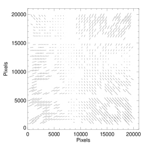
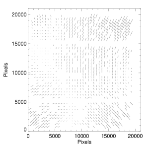
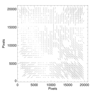
A visual inspection of the MegaPrime PSF (Fig.2) shows that the PSF anisotropy has significant variation over the field and may also be very large at the boundaries. The PSF correction is therefore a critical step and its reliability demands careful verifications. In addition to the usual B-mode analysis shown in the next section, in this section we carry out several analyses of the systematics.

The quality of the PSF correction and its homogeneity over the Megacam field camera can be assessed by comparing the mean star ellipticity before and after PSF correction (Fig.3). The average stellar ellipticities $\langle e_{t}\rangle$ and $\langle e_{r}\rangle$ are plotted as a function of the radial distance from the center of the field, $r$. It is interesting to note that the radial ellipticity component degrades much more and much faster than the tangential ellipticity. However, the PSF correction done by the PSF mapping is very good, for each Deep field. After correction, the dispersion of star ellipticities is about 2 $\times$ 10^-3 at any point of the camera. There is no significant change in the residual error as function of position. The small increase in the fluctuation of star shapes at very small distances is due to higher Poisson noise: each radial bin has the same width, so the innermost circle encompasses the smallest area and contains fewer stars than the others.

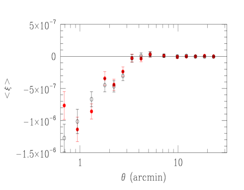
Finally, we checked the residual amplitude of the shape correlation function between corrected stars. We found is to be two order of magnitude smaller than the expected lensing signal at all scales probed by this work (Fig. 4).

The tests discussed above only guarantee that the PSF correction is excellent in the neighborhood of selected stars or on angular scales larger than, or close to, the mean angular distance between stars. In regions where no stars were selected or on small scales, the local PSF correction residuals may be larger than the average. A useful test of systematic residuals on small scales has been proposed by Bacon et al. (2003) and Heymans et al. 2005b . Assuming the PSF model derived from stars and applied to galaxies is unable to remove all systematic contributions, the star-galaxy cross correlation will be non-zero and may vary as function of angular scale. If the residual is small, Bacon et al. (2003) showed the systematic residual can be expressed as follows:

$$\xi_{sys}=\frac{\langle e_{*}\;e_{gal}\rangle^{2}}{\langle e_{*}\;e_{*}\rangle}\ ;$$ (22)

where $e_{gal}$ is the corrected galaxy ellipticity and $e_{*}$ is the uncorrected star ellipticity. We use the $\xi_{sys}$ to compute the contribution of systematics for both top-hat and compensated filter. Fig. 5 shows they are consistent with zero at all scales between 0.5 arc-minute to 30 arc-minutes. This confirms that residual systematics are negligible in the Megacam Deep fields.

Figure 3: Bottom panels show the mean tangential (left panel) and radial (right panel) uncorrected stellar ellipticity as a function of the distance to the center of the camera for D1rT001 (filled triangles ), D3rT001 (filled squares) and D4rT001 (filled circles) fields. Top panels show the same quantities after PSF correction.

Figure 4: E-modes (red filled circles ) and B-modes (black open circles) top-hat two point statistics of corrected stars show the smallness of residual PSF systematics.

Figure 5: Two-point signal statistics(red filled circles):top-hat (bottom) and $M_{ap}$ (middle) correlation function (top), compared with residual systematics (black open circles). Signal error bars are statistical ones.

5.2 Independent analysis of $r^{\prime}$ and $i^{\prime}$ data

The robustness of cosmic shear signal can also be assessed by comparing results obtained using different filters for the same galaxy sample. Because gravitational lensing is achromatic, we expect the shape and amplitude of cosmic shear to be identical for data taken in different filters. Any significant difference between two bands provides a diagnostic of the PSF corrections. A first attempt at comparing shear measurements in different filters was made by Kaiser et al. (2000) using the CFHT12K camera. The $I$ and $V$ bands showed significantly different signals that were inconsistent with the change in redshift distribution between the two filters.

The Deep photometry provides a sample of the same galaxies detected in different filters, so the signal is expected to be the same. However, these filters have different depths, and the shallowest colours do not have enough galaxies to allow a comparison of the signal between all colours using the same galaxies. This limitation affects mainly the $u^{*}$ and $g^{\prime}$ bands. Furthermore, these bands are more sensitive to atmospheric dispersion than other filters. We expect their PSF anisotropy to be larger than for $r^{\prime}$, $i^{\prime}$ and $z^{\prime}$ bands and its correction may also depend more on the relative differences between the averaged spectral energy distributions of stars used for the PSF calibration and of galaxies. Hence, $u^{*}$ and $g^{\prime}$ are not well suited for weak lensing analysis. The comparison between the $r^{\prime}$ and the $z^{\prime}$ bands doesn’t give many informations because of the limited size of the matched sample. We therefore decided only to focus on the comparison between $r^{\prime}$ and $i^{\prime}$ bands.

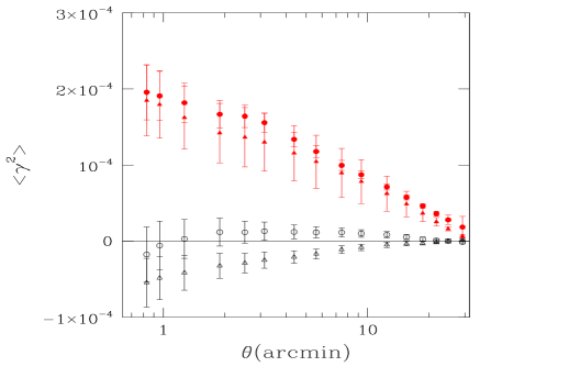
We computed the two-point statistics using the same objects in $i^{\prime}$-band and $r^{\prime}$-band in the D1 and D3 fields only. As reported before, D4 was discarded from this study because it shows higher systematic residuals in $i^{\prime}$ bands than the two other fields. It is worth noting that both $r^{\prime}$ and $i^{\prime}$ band images have been processed (flat fielding, astrometric and photometric calibrations, image selection, image stacking) in a totally independent way. The only correlations between the two samples are the software tools and the pipeline scheme used at Terapix.

The $r^{\prime}$ and $i^{\prime}$ ellipticity catalogues have been computed and PSF-corrected independently, starting from the $r^{\prime}$ and $i^{\prime}$ T0001 stacked images. The galaxy cross-identification is done at the very end of the processing to compare the results. Fig. 6 shows the comparison of the $E$- and $B$-modes of the top-hat shear variance for both the $i^{\prime}$ and $r^{\prime}$ data sets. The error bars are estimated as the quadrature sum of the statistical and the systematic error $\xi_{sys}$ defined by Eq.(22). The amplitude of the latter is bigger in the $r^{\prime}$ band as shown by the residual B-modes in this filter. The $r^{\prime}$ and $i^{\prime}$ bands results are remarkably similar, both in shape and amplitude, they agree to within $1\,\sigma$ at all scales.

Figure 6: Top-hat variance of the E-modes in the i’-band (red filled circles) and in the r’-band (red filled triangles) for the same data set. Top-hat variance B-modes in the i’-band (black open circles) and in r’-band (black open triangles).

6 Characterization of the shear signal

6.1 Two point statistics

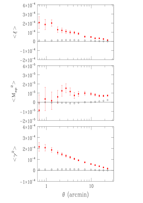
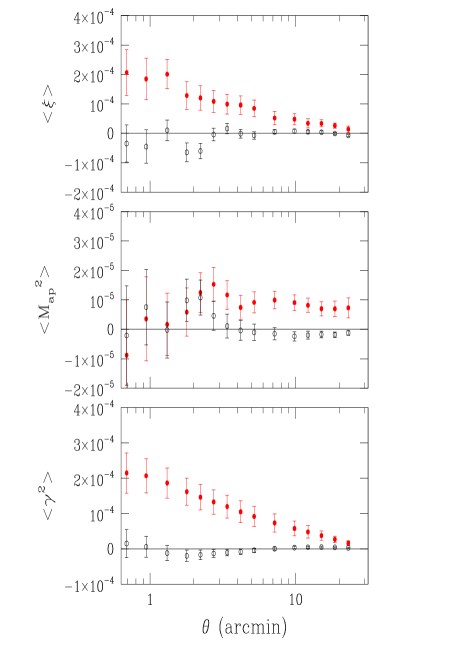
The ellipticity correlation functions $\xi_{+}(r)$ and $\xi_{-}(r)$ are measured from the weighted mean of all pairs with angular separation $r$. The correlation function is computed using equations (11) and (12). The $M_{ap}$ and the top-hat statistics are also computed as a function of the correlation functions $\xi_{+}(r)$ and $\xi_{-}(r)$ following Schneider et al. (2002) and Crittenden et al. 2001b . Fig.7 shows the two-point statistics for the three deep fields D1, D3 and D4. Error bars including statistical noise and cosmic variance are computed from the $\xi_{+}(r)$ and $\xi_{-}(r)$ as described in Schneider et al. (2002).

The cosmic variance contribution is computed using the CFHTLS T0001 Deep survey properties: an effective density (after masking) of $20\,gal/arcmin^{2}$, an effective area of $2.1\,deg^{2}$, and an ellipticity dispersion per ellipticity component of $0.3$ (the latter was measured from the corrected ellipticity). However, the error calculation described in Schneider et al. (2002) is only valid for a single connected field with a number density of $n$ equally-sized galaxies. We therefore replace the statistical error component by the Poisson noise measured from the data, using the weights (computed as described above) and positions of each galaxy. For the top-hat variance and the correlation function, the free integration constant is chosen so that the B-modes on scales between $15$ and $25$ arc-minutes vanish. Although its amplitude is meaningless, one can see that the B-mode is flat and stable over that range of angular scales.

In contrast, the $M_{ap}$ statistic does not have an undetermined integration constant (as explained previously), so the B-mode amplitude is a physical property. Fig.7 shows the presence of B-modes. Note that the $M_{ap}$ filter for a given size $\theta$ is mostly sensitive to scales around $\simeq\theta/5$. This explains why the other two-point statistics do not show B-modes at the same scales. The B-mode at such small scales may result from intrinsic alignment of galaxies (King & Schneider (2002); Heymans & Heavens (2003)) or from the correlation between intrinsic ellipticity and shear (Hirata & Seljak (2004)). If these systematics are real, we expect to correct them in future work by using the photometric redshifts. A further investigation confirms that the B-modes come from weak objects (i.e. $25.0<r^{\prime}_{AB}<25.5$), and that a magnitude cut that rejects objects with magnitude fainter than $25.0$ gives zero B-modes at all the scales, even for the $M_{ap}$ statistic. However, we keep these objects in our catalogues because a deep sample will be necessary to study the evolution of signal with redshift. In addition, the presence of B-modes at small scales will taken into account when we estimate cosmological parameters.

Figure 7: Two-point statistics for all the three fields combined. Red filled circles show E-modes, black open circles show B-modes. E-mode error bars include the statistical error and the cosmic variance contribution, while B-modes are affected only by statistical error.

6.2 Evolution of signal with redshift

The cosmological nature of the two-point statistical signal can be established by comparing its amplitude as function of source redshifts with theoretical expectations of the gravitational instability paradigm and the gravitational lensing theory (Bernardeau et al. (1997); Jain & Seljak (1997)). To first order, the signal should increase as $z_{s}^{1.5}$ (Bernardeau et al. (1997); Jain & Seljak (1997), so even a rough separation of galaxies into low- and high-redshift populations should split the cosmological lensing signal accordingly.

The CFHTLS T0001 data sets are well suited for this analysis. The observations can be used to sample the high redshift universe up to $z\simeq 1$. There are enough of galaxies to divide into two subsets based on their estimated photometric redshifts.

Photometric redshifts were measured using the hyper-z public software (Bolzonella, Miralles & Pelló (2000)). hyper-z uses the multi-band photometric data of a galaxy to derive its most likely redshift and spectral energy distribution (SED) based on the Bruzual & Charlot evolution models (Bruzual & Charlot (1993)).

We used the D1 and D3 $u^{*}$, $g^{\prime}$, $r^{\prime}$, $i^{\prime}$ and $z^{\prime}$ images and the D4 $u^{*}$, $g^{\prime}$, $r^{\prime}$, $i^{\prime}$ images (the D4-$z^{\prime}$ stacked image is missing in T0001). Photometric catalogues were produced by the SExtractor software. All galaxies were first detected in the $r^{\prime}$ band reference image. Magnitude and colours of galaxies are then computed using the $r^{\prime}-$center positions and inside an aperture scaled according to the size of each galaxy in $r^{\prime}$-band. The $\chi^{2}$ minimization was performed assuming magnitude errors derived from SExtractor, which range between $\Delta mag=0.03$ and $\Delta mag=0.1$ in all bands.

Fig. 8 shows the photometric redshift distribution of the galaxies in D1 field down to $i^{\prime}=24.0$. This subsample can be compared with the VVDS spectroscopic redshift distribution obtained from 11000 spectra in the same region (Le Fèvre et al. (2005)). There are no apparent discrepancies that would make the separation into photometric low- and high-redshift galaxies unreliable. Beyond $i^{\prime}=24.0$, large spectroscopic redshift samples are not yet available, but we don’t have any reason to believe that our photometric redshift accuracies will degrade significantly for the $i^{\prime}<24.0$ sample.

Figure 8: Density of galaxies of D1 field as a function of photometric redshift.

Table 2: Mean photometric redshift in magnitude bins.

magnitude bin	mean redshift
$18.5\leq i_{AB}\leq 24$	$<z>=0.850$
$19.0\leq i_{AB}\leq 24$	$<z>=0.853$
$19.5\leq i_{AB}\leq 24$	$<z>=0.858$
$20.0\leq i_{AB}\leq 24$	$<z>=0.865$
$20.5\leq i_{AB}\leq 24$	$<z>=0.876$
$21.0\leq i_{AB}\leq 24$	$<z>=0.892$
$21.5\leq i_{AB}\leq 24$	$<z>=0.913$
$22.0\leq i_{AB}\leq 24$	$<z>=0.942$
$22.5\leq i_{AB}\leq 24$	$<z>=0.981$
$23.0\leq i_{AB}\leq 24$	$<z>=1.035$
$23.5\leq i_{AB}\leq 24$	$<z>=1.100$

The cosmic shear catalogue can therefore be split into two samples with equal numbers of galaxies at high and low redshifts with reasonable confidence and can be compared with cosmological predictions. Poisson noise is therefore similar in the two subsamples, but photometric redshift errors are expected to be larger in the high-redshift tail.

Figure 9: Top-hat variance for “high-$z$” subsample (red filled triangles) and “low-$z$” subsample” (red filled circles). B-modes for the two subsamples are also shown. Error bars include statistical noise and cosmic variance. The data are compared with theoretical fiducial model ($\Omega_{m}=0.3$, $\Omega_{\Lambda}=0.7$, $\sigma_{8}=0.88$ and $h=0.7$ ) and source distribution $n(z)$ modeled by Eq.13, with $\alpha=1.98$, $\beta=0.66$ and $z_{s}=0.0981$. The low-$z$ source selection is simulated using $n(z)$ between $0.3<z<1.2$ and zero otherwise (bottom line). Likewise, the red filled triangles and the black open triangles are the E- and B-modes of the “high-$z$” sample. The data are compared with the same theoretical model with a high-$z$ source selection simulated using $n(z)$ between $z>0.8$ and zero otherwise. Shaded areas show models within $z_{s}=0.0981^{+0.013}_{-0.011}$ that represent the $1\sigma$ error region on $z_{s}$ as derived from the likelihood parameter estimation.

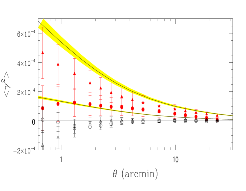
Fig. 9 shows the top-hat shear variance measured for the two populations. The low-$z$ sample ranges in $0.3\lower 2.15277pt\hbox{$\;\buildrel<\over{\sim}\;$}z\lower 2.15277pt\hbox{$\;\buildrel<\over{\sim}\;$}1.$, while the high-$z$ galaxies have $z\lower 2.15277pt\hbox{$\;\buildrel>\over{\sim}\;$}1.0$. Error bars include Poisson noise and cosmic variance (see Sect. 4.2). The difference between the two samples demonstrates the cosmological nature of the signal. An indicative comparison of signals with theoretical predictions is also plotted.

The relative lensing amplitude for the two source galaxy populations is less sensitive to cosmic variance fluctuations, and agrees with the predictions.

Contamination by galaxies with incorrect photometric redshifts is likely important, in particular for the faintest galaxies and the high-$z$ tail ( further informations about degeneracy of photometric redshifts in the case of missing infrared bands can be found on hyper-z user’s guide).

In spite of potential contamination by incorrect photometric redshifts, the cosmological imprint of large-scale structure detected in the Deep CFHTLS data shows that MegaPrime is suitable for cosmic shear studies. Fig. 9 also demonstrates that the CFHTLS Deep survey has promising potential for tomographic studies that explore the evolution of the dark matter power spectrum with look-back time.

7 Parameter estimation

7.1 Derivation of the likelihood function

In this Section, we describe the estimation of cosmological parameters. In a subsequent paper, we will perform a complete parameter estimate, combining weak lensing with other cosmological probes. Therefore, here we limit the analysis to the normalization of the mass power spectrum ($\sigma_{8}$) and matter density ($\Omega_{m}$) measurements. The shape parameter $\Gamma$ is given by the Cold Dark Matter paradigm $\Gamma=\Omega_{m}\leavevmode\nobreak\ h$, where $h$ is the reduced Hubble constant. We allow the characteristic redshift of the source distribution to vary around the best fit that will be described in the next sub-section.

To measure cosmological parameters, we adopt a maximum-likelihood method. Let $d_{i}$ be the input data vector (i.e. the top-hat shear variance as a function of scale $\theta_{i}$), and $m_{i}(\Omega_{m},\sigma_{8},n(z))$ the prediction, function of the parameters to be estimated. The likelihood function of the data is then:

$${\cal L}={1\over(2\pi)^{n}|{\bf C}|^{1/2}}\exp\left[(d_{i}-m_{i}){\bf C}^{-1}(d_{i}-m_{i})^{T}\right],$$ (23)

where $n=16$ is the number of angular scale bins and ${\bf C}$ is the $16\times 16$ covariance matrix of the top-hat shear,

$$C_{ij}=\langle(d_{i}-m_{i})^{T}(d_{j}-m_{j})\rangle,$$ (24)

and ${\bf C}$ can be decomposed as ${\bf C}={\bf C}_{n}+{\bf C}_{s}$, where ${\bf C}_{n}$ is the statistical noise and ${\bf C}_{s}$ the cosmic variance covariance matrix.

As discussed above, the matrix ${\bf C}_{s}$ is computed according to Schneider et al. (2002), assuming an effective survey area of the CFHTLS Deep fields: $2.1$ square degrees, a number density of galaxies $n_{gal}=20/arcmin^{2}$, and an intrinsic ellipticity dispersion of $\sigma_{e}=0.3$ per component.

The cosmic variance is computed assuming Gaussian statistics. While this assumption becomes inappropriate on small angular scales, errors on such scales are dominated by the statistical noise contribution, so the Gaussian approximation remains an excellent one (Van Waerbeke et al. (2002)). The covariance matrix components are derived for a fiducial cosmological model corresponding to the best fit of WMAP data proposed by Spergel et al. (2003): $\Omega_{M}=0.3$, $\Omega_{\Lambda}=0.7$, $\sigma_{8}=0.88$, $\Gamma=0.21$ (the reduced Hubble constant is $h$=0.7). The $B$-mode is calibrated by marginalizing around $B=0$ within the 1$\sigma$ interval.

7.2 Parameter estimation

The source redshift distribution is calibrated using the Hubble Deep Field (HDF) catalogues (Fernández-Soto et al. (1999)), which provide a more accurate estimate of redshift in absence of infrared data in CFHTLS fields. It turns out that the F606 filter of WFPC2 is a good match to the Megacam r’ filter within our $1\,\sigma$ magnitude error. We select all galaxies with $21.5<r^{\prime}<25.5$. The Hubble Deep Fields provide a sample at high redshifts that overlaps with the redshift range expected for the CFHTLS Deep fields.

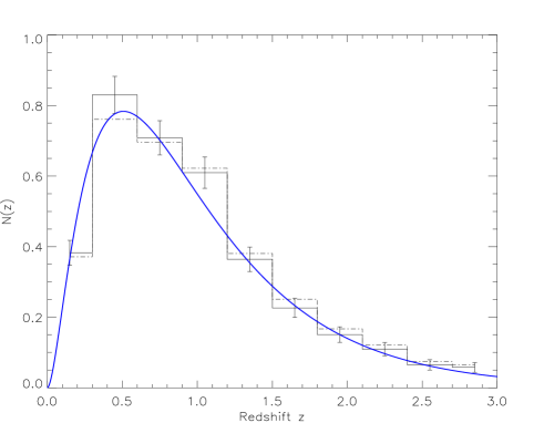
We use the source redshift distribution model of Eq.12 and perform a $\chi^{2}$ fit, allowing the parameter $z_{s}$ to vary. We then identify the $\pm 1\sigma$ and $\pm 2\sigma$ uncertainties, which we marginalized over in the cosmological parameter estimation. We find $\alpha=1.9833$, $\beta=0.6651$, $z_{s}=0.0981^{+0.013+0.021}_{-0.011-0.016}$. Figure 10 shows the unnormalized weight in magnitude slices in the Deep catalogues. The effect of down-weighting faint galaxies is taken into account in the source redshift estimation. Figure 11 shows the best fit model and the underlying photometric redshifts from the Hubble Deep Fields (solid line). Error bars are Poisson errors. The dashed-dotted line on Figure 11 shows the redshift distribution one would have if we ignore the weighting. The best fit redshift distribution model has a mean source redshift of $\approx 1.01$, nearly $0.2$ higher in $z$ than the Wide survey (Hoekstra et al. 2005).

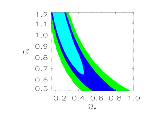
The constraints on $\Omega_{m}$ and $\sigma_{8}$ are obtained after marginalization of the reduced Hubble constant $h\in[0.6,0.8]$ and over the $\pm\leavevmode\nobreak\ 2\sigma$ limits of the source redshift parameter $z_{s}$. The resulting constraints in the $\Omega_{m}$-$\sigma_{8}$ plane are given in Figure 12. This figure shows that the CFHTLS Deep field gives constraints as good as previous lensing measurements, despite its small field of view. This is the consequence of the larger fraction of high redshift galaxies, which are more strongly lensed. Using the Peacock & Dodds (1996) non-linear scheme, we obtain $\sigma_{8}=0.94\pm 0.15\pm 0.20$ ($\pm\leavevmode\nobreak\ 1\sigma\pm\leavevmode\nobreak\ 2\sigma$) for $\Omega_{m}=0.3$. Error bars are the one and two $\sigma$ errors respectively. The Smith et al. (2003) halo model gives $\sigma_{8}=0.90\pm 0.14\pm 0.20$, which agrees with previous normalization measurements. The similarity between the result obtained using the Peacock & Dodds and that using the halo fitted model is not surprising. Indeed, on scales $\lower 2.15277pt\hbox{$\;\buildrel>\over{\sim}\;$}1^{\prime}$, which dominate our signal, the difference between the two models of power spectrum is $\lower 2.15277pt\hbox{$\;\buildrel<\over{\sim}\;$}5\%$. On smaller scales, we would expect an increasing discrepancy between these different ways to estimate $\sigma_{8}$.

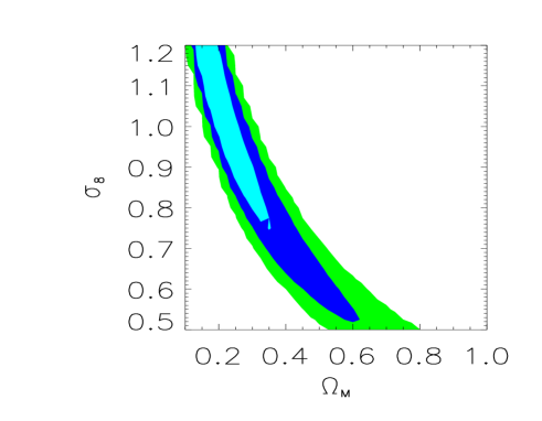
We then measure $\sigma_{8}$ by combining these constraints with those obtained on the CFHTLS Wide survey (see Hoekstra et al. 2005 for the details). The result of this joint analysis is shown in Figure 13, and remarkably, the $\Omega_{m}$-$\sigma_{8}$ degeneracy is partially broken. This is the consequence of measuring the large and small scales simultaneously, as shown in Jain & Seljak (1997). For $\Omega_{m}=0.3$, we get $\sigma_{8}=0.89\pm 0.06\pm 0.12$ using Peacock & Dodds (1996) for the non-linear scheme and $\sigma_{8}=0.86\pm 0.05\pm 0.11$ for the halo model (Smith et al. 2003).

The power spectrum normalization is in very good agreement with results from medium-redshift and low-source-redshift weak lensing surveys (Hoekstra et al. (2002); Van Waerbeke & Mellier (2005)). It is remarkable that the parameters of the redshift distribution, which have been estimated from a different survey, are such that the normalization $\sigma_{8}$ lies within the errors of previous measurements. This is strong evidence that deep, medium and shallow lensing surveys are in cosmological agreement, hence reinforcing the ability of cosmic shear to probe the mass distribution at different redshifts and different scales.

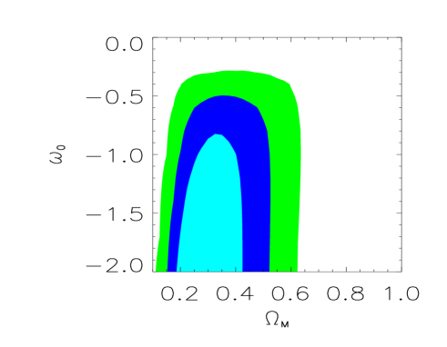
Weak lensing can also be used to constrain dark energy. Figure 14 show the upper limit on $w_{0}$, the constant equation of state parameter derived from the Deep data only. Here we used only the Peacock & Dodds non-linear prescription (a detailed discussion on non-linear power spectrum correction in the context of Dark Energy can be found in Hoekstra et al. (2005), which also includes a joint analysis of the Wide and Deep data). We obtain $w_{0}<-0.8$ at $1\sigma$, and the contours show that this result is independent of $\Omega_{M}$. This is particularly interesting because lensing combined with either cosmic microwave background (Jarvis et al. 2005) or supernovae will provide a strong constraint on the dark energy equation of state.

Figure 10: Plot of mean weight per galaxy as function of magnitude $21.5<r^{\prime}_{AB}<25.5$.

Figure 11: The histogram shows the photometric redshift distribution of $21.5<r^{\prime}_{AB}<25.5$ galaxies of Hubble Deep Field North and South used in this work. The central solid line is the best fit model. The solid line histogram is that magnitude weighted redshift distribution. The dashed-dot histogram shows the redshift distribution if the galaxies were not magnitude weighted.

Figure 12: $\Omega_{m}$ and $\sigma_{8}$ constraints with the Deep data only. The contours show 0.68, 0.95 and 0.999 confidence regions. Errors include statistical, covariance and residual systematic contributions. The models are pure Cold Dark Matter fit to the data, marginalized over the redshift distribution (see Section 7.2 for the details).

Figure 13: Same as Figure 12, combined with the CFHTLS Wide data (Hoekstra et al. 2005). For $\Omega_{m}=0.3$ we have $\sigma_{8}=0.86\pm 0.05$ at $1\sigma$ (see Section 7.2 for details of the error calculation).

Figure 14: Dark energy constraints from the Deep data only. Hidden parameters are marginalized using a flat prior over $\sigma_{8}\in[0.7,1.0]$, $h\in[0.6,0.8]$ and within the $\pm 2\sigma$ boundaries of the redshift parameter $z_{s}$ (see Section 7.2).

8 Summary and conclusion

This paper describes the first cosmic shear studies of CFHTLS Deep data using the T0001 CFHTLS release. It uses data collected in $u^{*}$, $g^{\prime}$, $r^{\prime}$, $i^{\prime}$ and $z^{\prime}$ with Megaprime/Megacam over the first year of the survey. Only between 1% and 15% of the Deep data are therefore in hand depending on the field and on the filter, and so the survey is still 2-3 magnitude below the final goal.

The T0001 data have been used to assess the capabilities of Megaprime/Megacam and to clarify the potential and the science drivers of the CFHTLS Deep survey for weak lensing studies.

The correction for PSF anisotropy works very well, showing that residual systematics are almost zero at all scales probed by a Megacam field. This is confirmed by the star-galaxy cross-correlation analysis. This also demonstrates that the CFHT-Elixir-Terapix calibration/reduction pipelines can deliver co-added images which have the required lensing quality. However, the presence of B-modes by weak objects at small scales should be further investigated.

The cosmic shear signal has been detected in the $r^{\prime}$-band. Its consistency and achromaticity has been checked by independent $r^{\prime}$- and $i^{\prime}$- analysis of the same data sets. We have presented results for three standard two-point shear statistics.

Thanks to the depth of the CFHTLS Deep sample, and using the photometric redshifts derived from the $u^{*}$, $g^{\prime}$, $r^{\prime}$, $i^{\prime}$ and $z^{\prime}$ images, the galaxy sample was split into low- and high-redshift sources, and the cosmic shear signal was measured on the two subsamples separately. Both subsamples show zero B-modes and the shear amplitude of the high-$z$ sample is clearly higher than the low-$z$ one, with a ratio in agreement with the cosmic shear predictions. The amplitude of the signals from the two subsamples are different from each other at all scales with a significance level higher than 5-sigma and their shapes follow theoretical expectations of $\Lambda$-CDM dominated universe. This strong evidence for the cosmological nature of the signal shows that the CFHTLS Deep data will allow us to explore the growth rate of cosmic shear signal with redshift, and hence the evolution of the dark matter power spectrum as function of lookback time.

Using only Deep data, and marginalizing over $h$ and the redshift of sources, we have derived constraints on $\sigma_{8}$ and $\Omega_{m}$. We show that the degeneracy between these two parameters is partially broken when the analysis is combined with data from Wide survey. Assuming $\Omega_{m}=0.3$, we found that $\sigma_{8}=0.89\pm 0.06$ for P&D and $\sigma_{8}=0.86\pm 0.05$ with the halo model, in excellent agreement with Van Waerbeke, Mellier & Hoekstra (2005) ($\sigma_{8}=0.83\pm 0.07$ ) and Hoekstra et al. (2002) ($\sigma_{8}=0.86\pm 0.05$ ). Likewise, we derive $w_{0}<-0.8$ using Deep data alone (see Hoekstra et al. (2005) for a deep+wide analysis).

Our results show that everything is in place to make a full scientific use the CFHTLS lensing data, and that soon with deeper Deep survey data and wider Wide survey data, we will able to provide the best cosmological constraints from weak lensing to date. In particular, we expect to explore the growth rate of structure from a tomographic cosmic shear measurement, and to better constrain cosmological models from the non-Gaussian features derived from a joint analysis of two-point and three-point statistics. The analysis of three-point statistics in CFHTLS data goes beyond the scope of this paper. Indeed, the Deep data used for this paper, is not wide enough for such a measurement. However, three-point statistics will be investigated using future samples both for the Deep and Wide survey.