Learning from the Scatter in Type Ia Supernovae

Abstract

Type Ia Supernovae are standard candles so their mean apparent magnitude has been exploited to learn about the redshift-distance relationship. Besides intrinsic scatter in this standard candle, additional scatter is caused by gravitational magnification by large scale structure. Here we probe the dependence of this dispersion on cosmological parameters and show that information about the amplitude of clustering, $\sigma_{8}$, is contained in the scatter. In principle, it will be possible to constrain $\sigma_{8}$ to within $5\%$ with observations of $2000$ Type Ia Supernovae. However, extracting this information requires subtlety as the distribution of magnifications is far from Gaussian. If one incorrectly assumes a Gaussian distribution, the estimate of the clustering amplitude will be biased three-$\sigma$ away from the true value.

Introduction.— Type Ia Supernovae (SNIa) are standard candles Baade (1938), with little dispersion around their mean luminosity. By measuring their apparent magnitudes, therefore, we can infer their distances from us. By observing supernovae at cosmological distances, we can measure the redshift-distance relationship and thereby extract information about cosmological parameters Colgate (1979); Tammann (1979); Goobar and Perlmutter (1995). Indeed, this method has supplied the most direct argument to date for dark energy Riess et al. (1998); Perlmutter et al. (1999) and serves as the basis for future proposals to probe the nature of dark energy, such as the Supernova Acceleration Probe (SNAP) Aldering et al. (2004).

The success of this program is based on the small intrinsic scatter in the SNIa luminosity. Various techniques have aided in the reduction of this scatter Phillips (1993); Riess et al. (1995, 1996); Perlmutter et al. (1997), which may be reduced even further in the future Aldering (2005). However, the intrinsic dispersion of SNIa luminosities is not the only source of scatter in the observations. Images at cosmological distances can be magnified (or de-magnified) by gravitational lensing produced by structure in the universe Kantowski et al. (1995); Frieman (1997); Wambsganss et al. (1997); Kantowski (1998). The amplitude of this cosmic dispersion depends on cosmological parameters Valageas (2000); Metcalf (1999): it increases with the matter density and the fluctuation amplitude. In principle, then, it might be possible to extract information about cosmological parameters not just by studying the mean apparent magnitudes of SNIa but also by looking at the scatter around the mean.

Since the mean is much more sensitive than the dispersion to the matter density, little additional information about $\Omega_{m}$ comes from the scatter. On the other hand, since the mean is completely independent of the fluctuation amplitude, it may be possible to use the cosmic dispersion profitably to infer $\sigma_{8}$, the rms amplitude of fluctuations on a scale of $8h^{-1}$Mpc. Ironically, in this age of precise parameter determination from measuring fluctuations in the microwave background and large scale structure, constraints on $\sigma_{8}$ are very loose . Current estimates Hoekstra et al. (2002); Spergel et al. (2003); Tegmark et al. (2004); Seljak et al. (2005); Viel et al. (2004); Sanchez et al. (2005); Jarvis et al. (2005); Viel and Haehnelt (2005) hover in the range $0.8-1.0$, and there is some evidence that $\sigma_{8}$ may be even larger than $1.0$ Komatsu and Seljak (2002); Bond et al. (2005) or as small as $0.6$ Viana et al. (2002). This leads us to ask whether upcoming supernovae searches can measure the cosmic dispersion and use it to constrain $\sigma_{8}$.

Distance Modulus.— The distance modulus of an unlensed source at redshift $z$ is

$$\mu_{0}=5\log_{10}\left[\frac{d_{L}(z)}{10\,{\rm pc}}\right]$$ (1)

where the luminosity distance in a flat universe (which is assumed throughout) is

$$d_{L}(z)=(1+z)c\int_{0}^{z}{dz^{\prime}\over H(z^{\prime})}.$$ (2)

Here $H(z)$ is the Hubble expansion rate, which in a flat universe with a cosmological constant and matter takes the form $H(z)=H_{0}[\Omega_{m}(1+z)^{3}+(1-\Omega_{m})]^{1/2}$, with $\Omega_{m}$ the matter density in units of the critical density. The current Hubble radius is $c/H_{0}=3000h^{-1}$Mpc, and we set $h=0.72$ throughout.

The actual distance modulus $\mu$ of a SNIa at redshift $z$ differs from that given in Eq. (1) because of the intrinsic dispersion $\delta\mu_{\rm int}$ – which is due to measurement errors, dispersion in SNIa luminosities, and absorbtion along the line of sight – and because of the cosmic dispersion $\delta\mu_{\rm cos}$ due to gravitational lensing:

$$\mu=\mu_{0}+\delta\mu_{\rm int}+\delta\mu_{\rm cos}.$$ (3)

The mean of each of these two effects is zero, so $\langle\mu\rangle=\mu_{0}$. The variance of $\delta\mu_{\rm cos}$ depends on the redshift of the source and can be related to the variance of the convergence $\kappa$

$$\kappa\equiv\frac{3\Omega_{m}H_{0}}{2\,c}\int_{0}^{\chi_{s}}d\chi[1+z(\chi)]\frac{\chi(\chi_{s}-\chi)}{\chi_{s}}\,\delta({\chi}),$$ (4)

by the following integral along the line of sight over all Fourier modes of the power spectrum:

$$\sigma_{\rm cos}^{2} = \left[\frac{5}{\ln(10)}\right]^{2}\langle\kappa^{2}\rangle$$ (5)

$$= {225\,\pi\Omega_{m}^{2}H_{0}^{4}\over 4[\ln(10)]^{2}}\int_{0}^{\chi_{s}}d\chi[1+z(\chi)]^{2}\frac{\chi^{2}(\chi_{s}-\chi)^{2}}{\chi_{s}^{2}}$$

$$\times\int_{0}^{\infty}{dk\over k^{2}}\Delta^{2}(k,z(\chi)).$$

Here, $\chi$ is the comoving distance to redshift $z$, $\chi_{s}\equiv\chi(z_{s})$ denotes the comoving distance to the source, $\delta(\chi)$ is the overdensity at comoving distance $\chi$ and $\Delta^{2}=k^{3}P(k,z)/2\pi^{2}$ is a dimensionless measure of the power.

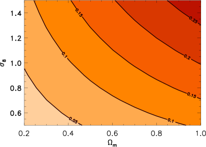
Figure 1: Cosmic dispersion of SNIa distance modulus, $\sigma_{\rm cos}$, as a function of cosmological parameters. Source here is at $z=1$.

The integrand in Eq. (5) is here evaluated using the algorithm of Smith et al. Smith et al. (2002) to generate the dark matter power spectrum as a function of redshift. Fig. 1 shows the cosmic dispersion in the distance modulus as a function of the matter density $\Omega_{m}$ and the fluctuation amplitude $\sigma_{8}$. Our results agree with previous determinations Hamana and Futamase (1999); Valageas (1999). The curves of constant $\sigma_{\rm cos}$ have a familiar shape: typically the amount of lensing increases if either the matter density or the fluctuation amplitude goes up.

It is important to stress, however, that the cosmic dispersion $\sigma_{\rm cos}$ does not fully characterize the distribution of magnifications and therefore of the distance moduli. In particular, it has been shown Valageas (1999) that the convergence – and consequently also the magnification – is not distributed according to a Gaussian distribution. As we show below, incorrect assumptions about the underlying distribution can lead to a bias in $\sigma_{8}$.

Projected Constraints on $\sigma_{8}$.— The aim of the present work is to extract information on the cosmological parameters not only from the mean value of $\mu$ but also from its dispersion. This operation is complicated by the fact that cosmic and intrinsic dispersion add in quadrature, and therefore separating one from the other requires some care Metcalf (1999). In what follows the only assumption made about the intrinsic dispersion is that it is independent of redshift. The conclusions presented below will therefore be strengthened if prior knowledge about the intrinsic dispersion can be used or weakened if the intrinsic dispersion varies with redshift (unless this variation is understood).

Figure 2: Dispersion in distance modulus of a SNIa as a function of its redshift for $\Omega_{m}=0.3$ and $\sigma_{8}=0.9$. The two sources of dispersion – internal and cosmic – add in quadrature. Throughout this work, we assume that the intrinsic dispersion is constant and equal to $0.1$. Points with error bars are projections for a future experiment which measures $2000$ supernovae in the redshift range $0.5$-$1.7$. Since the noise, $\sigma_{\rm int}$ is unknown, the signal, $\sigma_{\rm cos}$, is difficult to extract from the sum.

Fig. 2 shows the variation of the cosmic dispersion with redshift. As expected, there is more lensing for more distant sources, so the cosmic dispersion increases with $z$ (roughly as $[1+z]^{2.5}$). This characteristic increase makes it possible to distinguish cosmic dispersion from internal dispersion even without any foreknowledge of the magnitude of the latter. The expected errors on the total dispersion from a SNAP-like survey are also shown in Fig. 2. The error on the total variance (the dispersion squared) in a given redshift bin with $N$ supernovae is $(2/N)^{1/2}\sigma^{2}$ or of order $10^{-3}$ for an intrinsic dispersion of $0.1$ (which will be assumed throughout). However, to extract the cosmic dispersion, which is expected to contribute of order half the total dispersion at high redshifts, it is necessary to difference the variances in the different redshift bins. This doubles the noise on the variance (for two widely separated bins), and the signal is of order $\sigma_{\rm cos}^{2}\sim(0.05)^{2}$, only marginally larger than the noise. A careful weighting of the different redshift bins will then be necessary to extract the signal.

Likelihood analysis.— If the likelihood function was known, it would be straightforward to extract the cosmic signal optimally, for the maximum of the likelihood is the minimal variance estimator. A simple first guess for the likelihood is that $\delta\mu_{\rm int}$ and the convergence $\kappa$ are Gaussian distributed with variances $\sigma_{\rm int}^{2}$ and $\langle\kappa^{2}\rangle=\sigma_{\kappa}^{2}$ respectively. (The converegence $\kappa$ is considered because a fit for its distribution, which will be used below, has been derived in Ref. Wang et al. (2002).) Assuming that the lensing is uncorrelated Cooray et al. (2005), the total likelihood function is then the product of all the Gaussian distributions corresponding to all the observed supernovae. Here three parameters are considered: $\sigma_{8},\Omega_{m}$, and $\sigma_{\rm int}$. To project the errors on these parameters, we carried out the following simulation:

• Generate a supernova redshift randomly chosen to lie in the interval $0.5$-$1.7$.

• Using Eq. (1), compute the distance modulus of this SNIa in a universe with $\Omega_{m}=0.3$ and $\sigma_{8}=0.9$.

• With this set of cosmological parameters, compute the cosmic dispersion using Eq. (5).

• Draw $\delta\mu_{\rm cos}$ from the distribution resulting from the assumption that the underlying convergence is distributed according to a Gaussian with mean zero and variance $\sigma_{\kappa}^{2}$. Add $\delta\mu_{\rm cos}$ to the distance modulus.

• Draw $\delta\mu_{\rm in}$ from a Gaussian distribution with mean zero and variance $\sigma_{\rm int}^{2}$. Add $\delta\mu_{\rm in}$ to the distance modulus. This gives a final simulated value of $(z,\mu)$. Repeat these steps $2000$ times.

• For each point in the 3D parameter space ($\Omega_{m},\sigma_{8},\sigma_{\rm int}$), compute the likelihood of getting these $2000$ data points.

Once the likelihood function has been obtained in the 3D parameter space, projected errors on the cosmological parameters can be calculated by marginalizing over the unknown $\sigma_{\rm int}$. The resulting error matrix in $(\Omega_{m},\sigma_{8})$ space is roughly diagonal: because the mean distance modulus determines $\Omega_{m}$ extremely accurately, the errors on $\sigma_{8}$ and $\Omega_{m}$ are not correlated. That is, the mean distance modulus measurement breaks the degeneracy in the dispersion shown in Fig. 1. The projected 1-$\sigma$ error on $\sigma_{8}$ is $0.05$. This projected error agrees well with that obtained via a Fisher matrix analysis.

Up to this point, a Gaussian has been assumed for the distribution of the convergence. However, the distribution of the convergence is far from Gaussian Valageas (1999): it is skewed, so that most supernovae are demagnified while only a small fraction is highly magnified. Wang et al. Wang et al. (2002) used N-Body simulations to calibrate a phenomenological distribution based on the exact theoretical results obtained in Valageas (1999, 2000). Assuming this calibrated fit as the correct distribution for the convergence, we repeat the simulation with the following changes: (i) Once $\sigma_{\kappa}^{2}(z)$ is computed, $\delta\mu_{\rm cos}$ is drawn from the distribution obtained by assuming the results Wang et al. for the convergence; (ii) For each point in cosmological parameter space, the likelihood function is determined by convolving the distribution for $\delta\mu_{\rm cos}$ with a Gaussian of width $\sigma_{\rm int}$; (iii) To assess the impact that an erroneous assumption would have on the analysis of experimental data, the data generated with the non-Gaussian distribution are also (incorrectly) analyzed assuming a Gaussian distribution for both the convergence and the internal dispersion.

Fig. 3 shows the resulting likelihood function from one such simulation in the $\sigma_{8},\Omega_{m}$ plane after marginalizing over $\sigma_{\rm int}$. The shaded contours show that the maximum of the likelihood is shifted slightly from the true value; this is a reasonable statistical fluctuation. The 1-$\sigma$ error on $\sigma_{8}$ from this realization is $0.04$. It is slightly smaller than that obtained if the distribution were Gaussian. The shape of the distribution function for the convergence therefore encodes even more information about $\sigma_{8}$, information that could be mined if the distribution function were known accurately enough.

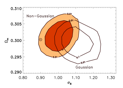
Figure 3: Projected constraints on the matter density and fluctuation amplitude from a SNAP-like survey. Contours show the ratio of the likelihood to its maximum value (true value is at starred point). The underlying probability distribution of the convergence is non-Gaussian. The two sets of contours correspond to analyzing the simulted data assuming the true distribution (shaded) or a Gaussian distribution (unshaded).

However, with the information encoded in this skewed distribution comes a caveat. An analysis which assumes that the distribution is Gaussian will produce a biased estimate of $\sigma_{8}$. The unshaded contours correspond to this assumption. For this realization, the Gaussian assumption clearly leads to a worse estimate of the best fit $\sigma_{8}$. To measure this bias, we ran one hundred simulations. On average, the best fit $\sigma_{8}$ was equal to the true value if the non-Gaussian analysis was used, but was biased with the Gaussian analysis. The average bias was $\Delta\sigma_{8}=0.12,$ three times larger than the anticipated statistical error. The skewness of the distribution – in particular, the few supernovae which have very large magnifications – can be explained in the Gaussian framework only if the dispersion is very large. Therefore, the Gaussian likelihood analysis will extract a value of $\sigma_{8}$ larger than the true value. The lesson is: if we want to extract $\sigma_{8}$, or any clustering parameter, from the dispersion of supernovae distance moduli, we must account for the non-Gaussianity of the lensing distribution. Note that this conclusion does not conflict with the recent results of Ref. Holz and Linder (2004). They showed that the non-Gaussianity of the distribution does not bias the extraction of the matter density or dark energy equation of state. We verify that the matter density, which is largely determined by the mean distance modulus, is unbiased in our simulations even if the Gaussian likelihood is used to analyze data generated with the non-Gaussian distribution. The clustering parameter, $\sigma_{8}$, though is biased because it is solely determined by the dispersion.

Conclusions.— Future SNIa surveys will be able to constrain the clustering amplitude $\sigma_{8}$ to within $5\%$. This is significantly better than current efforts and likely to be competitive even with future measurements. In order to extract an accurate value of $\sigma_{8}$, careful theoretical studies will need to pin down not just the cosmic dispersion as a function of cosmological parameters, but also the distribution of magnifications (especially at low redshift).

Besides the bias that can be induced by neglecting the non-Gaussianity of the convergence distribution, there are a number of systematics that could complicate this determination. First, the internal dispersion may vary with redshift: if this variation cannot be understood, at least some prior knowledge of the magnitude of the internal dispersion will be needed. Second, one might question the $\sigma_{8}-\sigma_{\rm cos}$ relationship. If only dark matter determined the lensing, then this connection would be relatively straightforward. However, cosmic dispersion is determined by structure on small scales. On the smallest scales, one must worry about the impact of baryons. Several groups  White (2004); Zhan and Knox (2004) have studied this recently in a different context and suggested that the power spectrum will be affected on scales $k>k_{f}=30$h Mpc^-1. If so, this would bias the determination of $\sigma_{8}$ at the ten percent level. Hydrodynamical simulations, though, should be able to reduce this systematic.