On the width and shape of gaps in protoplanetary disks

Abstract

Although it is well known that a massive planet opens a gap in a proto-planetary gaseous disk, there is no analytic description of the surface density profile in and near the gap. The simplest approach, which is based upon the balance between the torques due to the viscosity and the gravity of the planet and assumes local damping, leads to gaps with overestimated width, especially at low viscosity. Here, we take into account the fraction of the gravity torque that is evacuated by pressure supported waves. With a novel approach, which consists of following the fluid elements along their trajectories, we show that the flux of angular momentum carried by the waves corresponds to a pressure torque. The equilibrium profile of the disk is then set by the balance between gravity, viscous and pressure torques. We check that this balance is satisfied in numerical simulations, with a planet on a fixed circular orbit. We then use a reference numerical simulation to get an ansatz for the pressure torque, that yields gap profiles for any value of the disk viscosity, pressure scale height and planet to primary mass ratio. Those are in good agreement with profiles obtained in numerical simulations over a wide range of parameters. Finally, we provide a gap opening criterion that simultaneously involves the planet mass, the disk viscosity and the aspect ratio.

1 Introduction

The dynamical evolution of planets in proto-planetary disks has become a topic of renewed interest in the last decade, boosted by the discovery of extra-solar planets, and in particular of hot Jupiters. In fact, the observation of giant planets close to their parent stars argues for the existence of effective mechanisms of planetary migration, which can be found in the study of planet-disk interactions.

Several types of migration have been identified, depending on how the planet modifies the local density of the disk. Type I migration occurs when the planet is not massive enough to significantly alter the local density of the disk ; the planet migrates inward with a speed proportional to its mass (Ward, 1997). Type II migration corresponds to the case where the planet is so massive that it opens a clear gap in the disk ; the migration then depends on the viscous evolution of the disk (Lin and Papaloizou, 1986 a, b). Type III (or runaway) migration corresponds to planets with intermediate mass, which do not open a clear gap, but only form a dip around their orbits in the gas surface density profile ; under some conditions, their migration drift rate can grow exponentially, in a runaway process (Masset and Papaloizou, 2003).

The modification of the disk density is the result of the competition of torques exerted on the disk by the planet and by the disk itself. More precisely, the planet gives some angular momentum to the outer part of the disk, while it takes some from the inner part (Lin and Papaloizou, 1979 ; Goldreich and Tremaine, 1980). In doing so, it pushes the outer part of the disk outward and the inner part inward, and therefore tends to open a gap. However, the internal evolution of the disk, which tends to spread the gas into the void regions, opposes to the opening of the gap.

However, there is a lack of an analytical prediction of the gap profiles. Classically, the gap is considered to have a step function profile, with the edges located at the sites where the total gravity torque is equal to the total viscous torque. This is obviously an oversimplification. A more sophisticated approach has been recently presented by Varnière et al. (2004). They provide an analytic expression that describes the gap profile, by equating the viscous and gravity torques on any elementary disk ring. We will provide more details on this approach in section 2. The problem is that, when the viscosity is small, the viscous torque is small as well, and thus it cannot counterbalance the gravity torque. Consequently, in a low viscosity disk, a non-migrating planet should open a very wide gap, unlike what is observed in numerical simulations (see e.g. Fig. 1) : gaps do increase in width and depth as the viscosity decreases, but the dependence of the gap profile is less sensitive on viscosity in the numerical simulations than it is expected in theory.

Figure 1: Gap profiles created by a Jupiter mass planet, for different viscosities. The vertical axis represents the normalized azimuth-averaged density. The horizontal axis represents the distance to the primary in normalized units. Top panel : analytic curves obtained by matching the differential torques due to gravity and viscosity on each elementary ring of the disk. Bottom panel : numerical profiles obtained in simulations, after $1000$ planetary orbits for the three largest viscosities, and $5000$ orbits for $\log(\nu)=-5.5$ and $-6.5$.

The reason for this difference is that not all of the gravity torque is locally deposited in the disk. It is transported away by density waves (Goldreich and Nicholson, 1989 ; Papaloizou and Lin, 1984 ; Rafikov, 2002 ; see Appendix C). These waves are observed in simulations. In this situation, the viscous torque has to counterbalance only a fraction of the gravity torque, which yields narrower gaps than expected from the simple viscous/gravitational torque balance.

An evaluation of the fraction of the gravitational torque that is locally deposited at shock sites in the disk has been undertaken by Rafikov (2002). However he did not use his analysis to provide an analytic representation of the gap profile. Moreover, his calculation required several assumptions (the planet Hill radius had to be much smaller than the local disk height, the disk surface density was assumed to be uniform, etc.), which are not satisfied in the general giant planet case.

Here we introduce a novel approach. We follow a fluid element along its trajectory which, in the steady state, is periodic in the planet corotating frame. A flux of angular momentum carried by the density waves corresponds to a pressure torque acting on the fluid element, whose average over a synodic period is non-zero. In this work, we evaluate this averaged pressure torque, together with the gravity and viscous torques. The fact that the fluid element path is closed implies that these time averaged torques balance.

In section 3 we introduce the pressure torque, and we use numerical simulations to check that the gap structure is set by the equilibrium between the gravity torque and the sum of the viscous and the pressure torques. In section 4 we construct a semi-analytic algorithm and we get an expression to compute that gap profile. We compare our results with the profiles obtained in numerical simulation, and we discuss the merits and limitations of our method. In section 5 we use our algorithm to explore the dependence of the gap structure on disk viscosity and aspect ratio. We recover the trends observed in numerical simulations, namely the limited gap width in low viscosity disks and the filling of the gap with increasing viscosity and/or aspect ratio. Finally in section 6, we provide a gap opening criterion that simultaneously involves the viscosity, the scale height and the planet mass.

2 Gravity and Viscous Torques

In this section we revisit the calculation of the gravity and viscous torques mentioned in the Introduction. We show that considering them alone, as usually done, is not sufficient to achieve a quantitatively correct description of the gap profiles.

2.1 Notations

The disk is represented in cylindrical coordinates $(r,\theta,z)$, centered on the star, where the plane $\{z=0\}$ corresponds to the mid-plane of the disk. The disk viscosity $\nu$ and aspect ratio $(H/r)$ – where $H$ denotes the thickness of the disk – are assumed to be invariant in time and space. The equations of fluid dynamics are integrated with respect to the $z$-coordinate, so that $z$ disappears from the equations and only two dimensions are effectively used. This procedure introduces the concept of surface density $\Sigma$, which is defined as $\int_{-H}^{+H}\rho\,{\rm d}z$, where $\rho$ is the volume density in the disk.

In the theoretical analysis (but not in the numerical calculations) the disk is assumed to be axisymmetric, so that $\Sigma$ only depends on $r$. The angular velocity $\Omega$ is assumed to be Keplerian : $\Omega\propto r^{-3/2}$. The planet is assumed on a circular orbit around the star. The radius of its orbit is denoted $r_{p}$. The mass of the planet is denoted $M_{p}$ and its ratio with the mass of the central star $M_{*}$ is $q$. Normalized units are introduced, so that $M_{*}=r_{p}=1$ and the gravitational constant $G$ is also assumed to be unity. In the limit $q\to 0$, this sets the angular orbital velocity of the planet $\Omega_{p}=1$ and its period equal to $2\pi$.

2.2 Total torques

Usually, one considers the part of the disk extending from a given radius $r_{0}>r_{p}$ to infinity. The study of the part of the disk extending from 0 to $r_{0}<r_{p}$ is done in an analogous way. Two torques are evaluated. The first one is due to the disk viscosity and can be easily derived from the stress tensor in a Keplerian disk with circular orbits. The torque exerted on the considered part of the disk ($r>r_{0}$) by the complementary part is written (see for instance Lin and Papaloizou, 1993) :

$$T_{\nu}=3\pi\Sigma\nu{r_{0}}^{2}\Omega_{0}$$ (1)

Notice that more refined expression for perturbed disks with eccentric orbits have been proposed in the literature (see for instance Borderies et al. 1982), but they have not been used in the works that we review in this section.

The second torque comes from the gravity of the planet. It can be computed following two different approaches. In the first one (Goldreich and Tremaine, 1980 ; Ward, 1986), it is decomposed into the sum of the individual torques exerted at each Lindblad resonance. In the second approach (Lin and Papaloizou, 1979 ; Goldreich and Tremaine, 1980) it is obtained by computing the angular momentum change for fluid elements at conjunction with the planet, using an impulse approximation. The two approaches are known to give equivalent results. In the following, we use the expression from the impulse approximation :

$$T_{g}(\Delta_{0})=C\,q^{2}\Sigma{r_{p}}^{4}{\Omega_{p}}^{2}\left(\frac{r_{p}}{\Delta_{0}}\right)^{3}\ ,$$ (2)

where $\Delta_{0}=(r_{0}-r_{p})$. The above expression gives the torque exerted by the planet on a disk extended from $r_{0}$ to infinity. It is valid only for $|\Delta_{0}|>\Delta_{\rm m}$, where $\Delta_{\rm m}$ is the maximum of $H$ (the local thickness of the disk) and the Hill radius of the planet $R_{H}=(q/3)^{1/3}$ (Goldreich and Tremaine, 1980 ; Ward, 1997). The value of the numerical coefficient $C$ depends on the approach followed for the calculation of the torque. In the most recent and refined calculation, Lin and Papaloizou (1993) found $C=\frac{32}{243}[2K_{0}(\frac{2}{3})+K_{1}(\frac{2}{3})]^{2}\approx 0.836$ (where $K_{0}$ and $K_{1}$ are modified Bessel functions).

Classically, the gap is modeled as a step function profile in the disk surface density, with edges placed at a distance $\Delta_{0}$ from the planet orbit, with $\Delta_{0}$ given by the solution of the equation $T_{g}(\Delta_{0})=T_{\nu}$, and $T_{g}$ and $T_{\nu}$ given in (2) and (1). The maximal gravity torque is :

$$T_{g}(\Delta_{\rm m})\approx 0.836\,q^{2}\Sigma{r_{p}}^{4}{\Omega_{p}}^{2}\left(\frac{r_{p}}{\Delta_{\rm m}}\right)^{3}\ .$$

Thus, a gap can be opened only if :

$$\nu<0.0887q^{2}\frac{{r_{p}}^{4}{\Omega_{p}}^{2}}{{r_{0}}^{2}\Omega_{0}}\left(\frac{r_{p}}{\Delta_{\rm m}}\right)^{3}\ ,$$ (3)

otherwise $T_{\nu}$ is larger than $T_{g}$ and the gas overruns the planet. Condition (3) is equivalent to that given in Bryden et al. (1999), expressed as a constraint on the mass of the planet relative to the viscosity of the disk.

2.3 Differential torques and comparison with numerical tests

Differential torques.

Varnière et al. (2004) proposed a more refined approach to model the surface density profile in the gap. Their approach is based on a simple consideration : in equilibrium, when a steady state is reached, the gravity torque and the viscous torque must be equal on every elementary ring of the disk. The torques acting on elementary rings can be computed by differentiation relative to $r\equiv r_{0}$ of (1) and (2) :

$$\delta T_{\nu}(r)=-\frac{3}{2}\nu\Omega\left[\frac{r}{\Sigma}\frac{{\rm d}\Sigma}{{\rm d}r}+\frac{1}{2}\right]\left(2\pi r\Sigma\right)$$ (4)

$$\delta T_{g}(r)\approx 0.4\,q^{2}{r_{p}}^{3}{\Omega_{p}}^{2}r^{-1}\left(\frac{r_{p}}{\Delta}\right)^{4}\left(2\pi r\Sigma\right)$$ (5)

Matching $\delta T_{\nu}$ and $\delta T_{g}$ gives a differential equation in $\Sigma$ :

$$\frac{1}{\Sigma}\frac{{\rm d}\Sigma}{{\rm d}r}=\frac{\delta T_{g}(r)}{3\pi\nu{r}^{2}\Omega\Sigma}-\frac{1}{2r}$$ (6)

The integration of this equation gives the profile of the gap.

The top panel of Fig. 1 gives examples of the solution of Eq. (6) for several values of the viscosity, from strong ($\nu=10^{-3.14}$) to weak ($\nu=10^{-6.5}$). To compute them from (6), we have (i) assumed that the mass of the planet is $10^{-3}$ in our normalized units, (ii) imposed the boundary condition $\Sigma(r_{0}=3)=1/\sqrt{3}$ and (iii) assumed that the gravity torque is null in the horseshoe region, here approximated by : $r_{p}-2\,R_{H}<r<r_{p}+2\,R_{H}$. As a consequence of (iii) the surface density profile in the vicinity of the planet assumes an equilibrium slope proportional to $1/\sqrt{r}$, which makes $\delta T_{\nu}$ null. Notice that the slopes of the surface density at the edges of the gap do not depend on our assumptions (ii) and (iii), but are dictated solely by the differential equation (6). We remark that the profiles illustrated in the figure are the same as in Varnière et al. 2004, despite the fact that these authors consider the gravity torque as given by the sum of the individual Lindblad resonances. This again underlines the equivalence of the two approaches for the calculation of the gravity torque discussed in 2.2.

Numerical simulations.

We have tested the results of these analytic calculations using purely numerical simulations. For this purpose, we have used the 2D hydrodynamic code described in Masset (2000), and considered a Jupiter mass planet ($q=10^{-3}$) in a disk, whose initial surface density profile decays as $1/\sqrt{r}$, and $\Sigma(r_{p})=6.10^{-4}$ (the value of the minimal mass solar nebula at 5 AU (Hayashi, 1981)). The disk aspect ratio was fixed at $5\%$. The viscosity was chosen equal to the values used for the analytic computations, for direct comparison. In these simulations, the planet was assumed not to feel the gravity of the disk, so that it did not migrate. The grid used by the code for the hydrodynamical calculations extended from $0.5$ to $3$ (we remind that the planet location is $r_{p}=1$). The boundary conditions in $r$ are non-reflecting, which means that the waves behave as if they were propagating outside the boundaries of the grid. The angular momentum they carry is thus lost ; we have checked that the flux through the outer boundary represents only a negligible fraction of the total gravity torque (see Appendix C). The relative surface density amplitude perturbation at the outer boundary has been measured to be less than 5%. The size of the grid was 150 cells in radius and 325 cells in azimuth. The simulations were carried on for $1000$ planetary orbits, for viscosity down to $10^{-5.0}$ and $5000$ orbits for weaker viscosities. At these times, the profile of the gap does not seem to evolve significantly any more, as also found by Varnière et al. (2004).

Comparisons.

The results are illustrated in the bottom panel of Fig. 1. As anticipated in the introduction, we remark an evident difference with the analytic predictions. The simulated gap is much narrower than the one predicted by the analytic expression (6) for low viscosities ($\nu<10^{-6}$). At first sight, one might think that the discrepancy between the analytical and numerical solutions is due to the numerical viscosity (dissipation due to numerical errors) of the computer code. However, this is unlikely for the following reasons : (i) different gap profiles are observed for different viscosities, which shows that the simulation is not dominated by the numerical viscosity, as the latter should be the same in all simulations ; (ii) changing the resolution of the grid used in the numerical scheme, which changes the numerical viscosity, does not affect the gap profiles significantly ; (iii) different numerical schemes give consistent results (De Valborro, private communication).

As anticipated in the introduction, the problem with this analytical modeling is the assumption that the gravity torque is entirely deposited in each annulus of the disk. A condition for such deposition to happen is that $R_{H}\gtrsim H$ (Lin and Papaloizou, 1993). Thus, this is usually considered as a second independent criterion for gap opening, in addition to (3) (Bate et al., 2003). However, even if this condition is satisfied, a fraction of the gravity torque is still evacuated by the waves (Goldreich and Nicholson, 1989 ; Papaloizou and Lin, 1984 ; Rafikov, 2002). The problem is to evaluate this fraction. Below we show that it can be computed from a mean pressure torque acting on the fluid elements over their periodic equilibrium trajectories.

3 Pressure torque

Consider an arbitrary closed curve in the disk and a little tube around it. The rate of change of angular momentum of the matter in the tube is the sum of the differential flux of angular momentum through its boundaries (due to the advection of matter) and of the torques acting on it. From the Navier-Stokes equations, in addition to the gravity and viscous torques, there is a third torque due to pressure :

$$t_{P}=\oint{{c_{s}}^{2}}\frac{\partial\Sigma}{\partial\theta}{\rm d}\theta\ ,$$ (7)

where the integral is computed along the curve and we have assumed the usual state equation $P={c_{s}}^{2}\Sigma$ (with $c_{s}=H\Omega$ denoting the sound speed). If the tube is a ring centered at the origin $r=0$, the torque $t_{P}$ is equal to zero (on the ring, $r$ is constant and $\partial\Sigma/\partial\theta={\rm d}\Sigma/{\rm d}\theta$), while the differential flux of angular momentum is generally not zero. The latter is the flux carried by the pressure supported wave (Goldreich and Nicholson, 1989 ; see Appendix C). On the contrary, if one chooses a stream tube (i.e. a tube bounded by two neighboring streamlines), the differential flux is obviously zero (there is no flux of matter, by definition of stream tube), while $t_{P}$ is non zero in general. The latter is true because the streamlines are strongly distorted (see Fig. 2) so that $\Sigma\equiv\Sigma(r(\theta),\theta)$ and thus $\partial\Sigma/\partial\theta\neq{\rm d}\Sigma/{\rm d}\theta$. This shows that one can translate the angular momentum flux carried by the waves into a pressure torque, by a suitable partition of the disk in concentric tubes. Obviously the two approaches are equivalent as the physics is the same. However, working with stream tubes and pressure torques gives practical computational advantages. This is therefore the approach that we follow in this paper.

Below, we check that the gravity, pressure and viscous torques really cancel each other in the numerical simulations, once the steady state is reached.

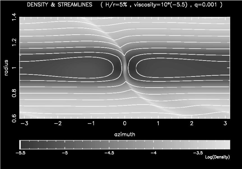
Figure 2: Disk surface density map in the vicinity of a gap opened by a Jupiter mass planet located at $(r_{p}=1,\theta_{p}=0)$. Light grey denotes high density and black low density, in a logarithmic scale. The white curves show some streamlines, in the frame corotating with the planet. They are followed from $\pi$ to $-\pi$ for $r>1$, and from $-\pi$ to $\pi$ for $r<1$, periodically. Two of them correspond to horseshoe orbits in the planet corotation region. Notice the strong distortion of the streamlines when they cross the over-density corresponding to the spiral wave (wake) launched by the planet.

3.1 Computation of the torques along the trajectories

The approach outlined above requires that the stream tubes are closed. In our simulations this is true at the steady state, because our boundary conditions preserve the initial radial velocity at the edges of the grid, which is null as a result of our choice for the initial disk density profile $\Sigma\propto 1/\sqrt{r}$. The calculation of the streamlines, which is done in Fourier space to ensure periodicity, is detailed in Appendix A. We remark that, in the steady state, the streamlines coincide with the fluid element trajectories.

Denoting the streamline by $r_{i}(\theta)$, we numerically compute the following expressions, which are the integrals of $(1/\Sigma)(r\textbf{F}_{\theta})$ with $\textbf{F}_{\theta}$ the azimuthal component of the force due to gravity, viscosity, or pressure respectively :

$$t_{g}(\theta)=\frac{1}{T_{i}(\theta)}\int_{\pi}^{\theta}r_{i}(\theta^{\prime})\frac{\partial\phi_{(r_{i}(\theta^{\prime}),\theta^{\prime})}}{\partial\theta^{\prime}}\left|\frac{d\theta^{\prime}}{\dot{\theta^{\prime}}}\right|$$ (8)

$$t_{\nu}(\theta)=\frac{1}{T_{i}(\theta)}\int_{\pi}^{\theta}\frac{1}{\Sigma_{(r_{i}(\theta^{\prime}),\theta^{\prime})}}r_{i}(\theta^{\prime})\textbf{F}_{\theta}^{\nu}(r_{i}(\theta^{\prime}),\theta^{\prime})\left|\frac{d\theta^{\prime}}{\dot{\theta^{\prime}}}\right|$$ (9)

$$t_{P}(\theta)=\frac{1}{T_{i}(\theta)}\int_{\pi}^{\theta}\frac{{c_{s}}^{2}}{\Sigma_{(r_{i}(\theta^{\prime}),\theta^{\prime})}}\frac{\partial\Sigma_{(r_{i}(\theta^{\prime}),\theta^{\prime})}}{\partial\theta^{\prime}}\left|\frac{d\theta^{\prime}}{\dot{\theta^{\prime}}}\right|$$ (10)

Here, $\phi$ denotes the gravitational potential of the planet, and $\textbf{F}_{\theta}^{\nu}=\frac{1}{r}\left[\frac{\partial}{\partial r}\left(r\bar{\bar{T}}_{r\theta}\right)+\frac{\partial}{\partial\theta^{\prime}}\bar{\bar{T}}_{\theta\theta}+\bar{\bar{T}}_{r\theta}\right]$, where $\bar{\bar{T}}=\left(\begin{array}[]{cc}\bar{\bar{T}}_{rr}&\bar{\bar{T}}_{r\theta}\\ \bar{\bar{T}}_{\theta r}&\bar{\bar{T}}_{\theta\theta}\end{array}\right)$ is the local viscous stress tensor for a Newtonian fluid : $\bar{\bar{T}}=2\Sigma\nu\left(\bar{\bar{D}}-(\frac{1}{3}\nabla\vec{v})I\right)$, where $\bar{\bar{D}}$ is the strain tensor and $I$ is the identity matrix. We integrate from $\pi$ to $\theta$, with $\pi>\theta\geqslant-\pi$, because we consider $r_{0}>r_{p}$, so that the angular velocity is negative in the corotating frame. The time required to reach $\theta$ from $\pi$ is denoted $T_{i}(\theta)$. Thus, as the trajectories coincide with the streamlines in the steady state, the expressions above describe the averaged torques felt by a fluid element that travels from the planet opposition to $\theta$.

In the following, we denote for simplicity by $t_{g}$, $t_{\nu}$, $t_{P}$ the expressions (8)-(10) evaluated at $\theta=-\pi$. The total torques acting on the stream tube centered around the considered streamline are simply the product of these quantities times the mass carried by the tube.

In the next paragraphs we give a brief description of the integrated torques (8)-(10) as functions of $\theta$, which are plotted in Fig. 3 for the streamline starting at $r=1.2$ at opposition with the planet.

Figure 3: Graphical representation of the expressions (8) (integrated gravity torque, bold short-dash curve), (9) (integrated viscous torque, bold dotted curve) and (10) (integrated pressure torque, bold solid curve). Their reference scale is reported on the left vertical axis. The streamline followed for their calculation is plotted in the planet corotating frame as a dashed curve at the top of the figure and can also be seen on Fig. 2, while the position of the planet is shown by a filled dot at the bottom ; the corresponding scale is reported on the right vertical axis. The thin solid curve shows the difference between the angular momentum measured along the streamline ($H(\theta)$ ), and the sum of the three integrated torques and of the initial angular momentum (${\cal H}(\theta)$ ). A small difference is almost impulsively acquired at the wake crossing, due to numerical approximations.

viscous torque :

The growth of the integrated viscous torque appears to be nearly linear with respect to the azimuth, leading to a total negative torque. We verified that on this streamline $t_{\nu}\approx\delta T_{\nu}/(2\pi\Sigma r)$, with $\delta T_{\nu}$ from (4). Thus, the viscous torque depends only on the radial relative derivative of the azimuthally averaged density $\frac{1}{\Sigma}\frac{{\rm d}\Sigma}{{\rm d}r}$. However, on streamlines that pass closer to the planet, the difference between $t_{\nu}$ and $\delta T_{\nu}/(2\pi\Sigma r)$ becomes more significant (see Fig. 6).

gravity torque :

The evolution of this integrated torque is not monotonic. The fluid element is first repelled by the planet, as a result of the indirect term in the gravitational potential. Then, when $\theta$ decreases below $\sim 0.5$, it starts to be attracted by the planet. The attraction becomes stronger and stronger as the fluid element approaches conjunction, namely as $\theta$ decreases to $0$. The integrated torque becomes negative. After conjunction, the planet tends to pull the fluid element toward positive $\theta$, giving a positive torque. As a result, the fluid element is rapidly repelled toward larger $r$, as one can see from the trajectory on Fig. 3. This is typical of the scattering of test particles in the restricted three body problem, which qualitatively justifies the impulse approach for the calculation of the gravitational torque, as in Lin and Papaloizou (1979).

However, Lin and Papaloizou’s calculation holds in the approximation $r\!\sim\!r_{p}$. By comparing the numerical estimate of $\delta T_{g}/(2\pi\Sigma r)$ with $\delta T_{g}$ given by Eq. (5), we find that the following expression, which has the same dependence in $\Delta$ and nearly the same numerical coefficient, but which distinguishes $r$ and $r_{p}$, provides a much more accurate representation of the gravity torque :

$$t_{g}=0.35\ q^{2}{r_{p}}^{\!5}\,{\Omega_{p}}^{\!2}\,r\left(\frac{1}{\Delta}\right)^{\!4}{\rm sgn}(\Delta)\ ,$$ (11)

In reality, $t_{g}$ depends on the exact shape of the streamlines, which in turn depends on the scale height and the viscosity (see Fig. 4 and 6). However, the difference is moderate and limited to the vicinity of the planet, so that in the following we use expression (11) for all cases.

We stress that expression (11) gives the torque exerted on the fluid element, which is generally not the torque deposited in the disk. In fact, even in the absence of viscosity, it does not correspond to the change of angular momentum of the fluid element, because some of the angular momentum is carried away by the pressure torque.

Figure 4: Absolute value of $t_{g}$ as a function of $r$, where $r$ is the distance to the central star at planet opposition of the streamline on which the gravity torque is integrated. The bold long-dashed curve is obtained from the simulation with $q=10^{-3}$, $(H/r)=5\%$, and $\nu=10^{-5.5}$, while the bold short-dashed curve corresponds to a more viscous case ($\nu=10^{-4.6}$). The solid line traces expression (11), which remarkably fits the results obtained in the less viscous case. The dashed-dotted curve traces expression (5), which shows that $\delta T_{g}\neq t_{g}$.

pressure torque :

The dependence of this torque on $\theta$ is simple to understand if one takes into account that : (i) the trajectories cross the wake immediately after the conjunction with the planet (Fig. 2) ; (ii) the wake is a strong over-density in the disk ; (iii) the pressure term $\partial\Sigma/\partial\theta$ makes over-densities repellent. Thus, as the fluid element approaches the wake, its azimuth $\theta$ decreasing in the corotating frame, the pressure rises and tends to push the fluid element back in the direction of increasing $\theta$. This gives a positive local torque and it explains the peak in the integrated pressure torque in Fig. 3. Then, after that the fluid element has crossed the wake, the pressure decreases as $\theta$ decreases. This leads to a negative local pressure torque. It corresponds to the fall after the peak on Fig. 3. The negative contribution is bigger than the positive one because of the asymmetry of the trajectory relative to the wake position, which is clearly visible in Fig. 5.

Clearly, the pressure torque must depend on the shape of the streamlines and on the surface density relative radial gradient, which govern the shape of the wake and its density enhancement. We return to this in section 4.

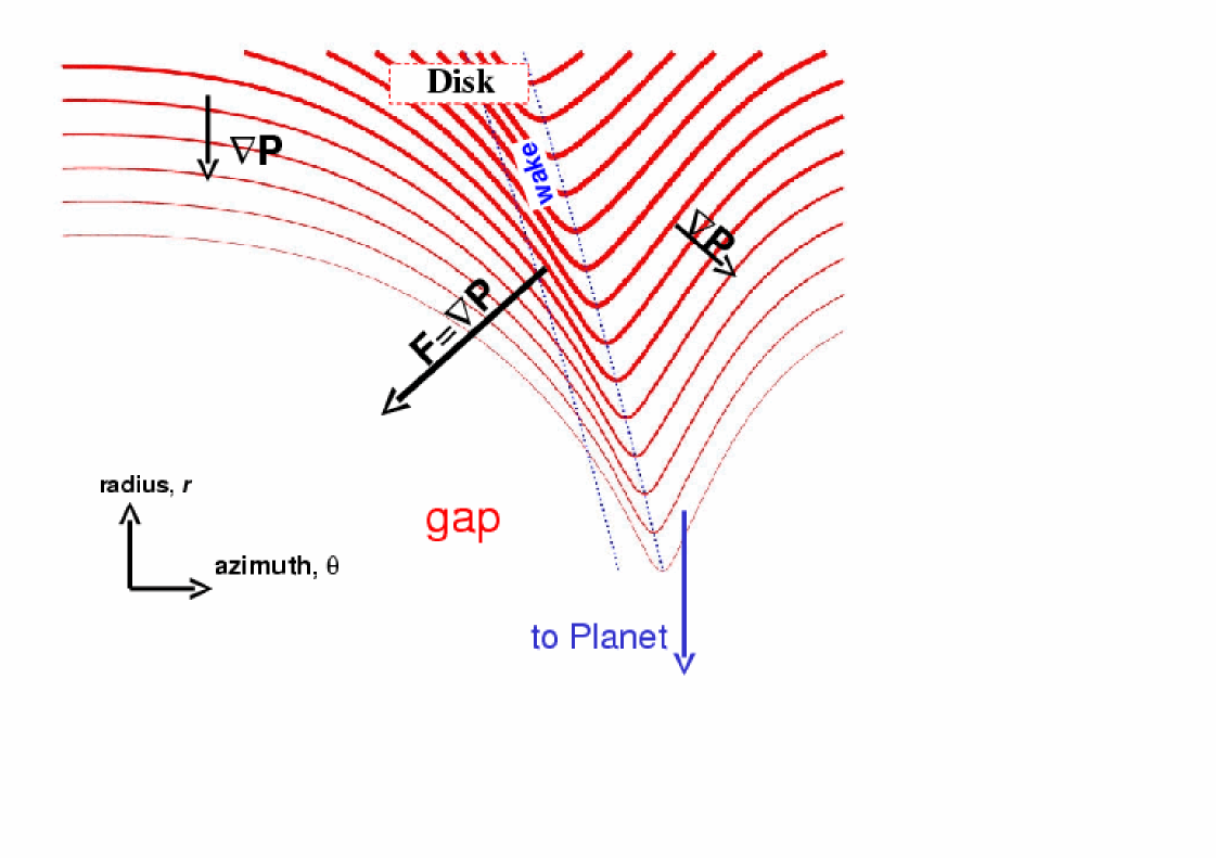
Figure 5: Sketch on the origin of the pressure torque. Here are drawn some streamlines, the width of which represents the mass carried by the corresponding streamtube. At the gap edge, the pressure gradient gives a force. The distortion of the streamlines at the wake leads to a large azimuthal component of this force, which gives a torque.

3.2 Torque balance at equilibrium

From Fig. 3 we remark that, at $\theta=-\pi$, the sum of the viscous and pressure torques is basically the opposite of the gravity torque. Therefore, the three torques approximately balance out.

Given the angular momentum $H$ of a fluid element at $\theta=\pi$, one can compute the angular momentum ${\cal H}(\theta)$ that it would have if its trajectory were governed exclusively by the three torques mentioned above : ${\cal H}(\theta)=H(\pi)+t_{g}(\theta)+t_{\nu}(\theta)+t_{P}(\theta)$. This can be compared with the local angular momentum on the trajectory $H(\theta)$, measured directly from the numerical simulation. In Fig. 3 the thin line shows $H(\theta)-\mathcal{H}(\theta)$. This function is zero for $\theta$ evolving from $\pi$ down to $\sim 0$, where the wake is crossed. At the wake crossing, a small kick is observed. Then, when $\theta$ evolves from the wake location to $-\pi$, the function $H(\theta)-\mathcal{H}(\theta)$ remains constant again. This confirms that the trajectory is essentially governed by the three torques mentioned above.

The small difference between $H$ and ${\cal H}$ (Fig. 3) could in principle be due to the pseudo-viscous pressure introduced in the simulation to avoid numerical instabilities (Lin and Papaloizou, 1986a), but we have verified that the effect of the latter is negligible. Thus, we conclude that it is a consequence of numerical errors, introduced by the grid discretization at the shock site. This numerical issue evidently prevents the three cumulative torques from balancing out perfectly at $\theta=-\pi$ : indeed, their sum is equal to $\mathcal{H}(-\pi)-H(-\pi)\neq 0$.

Figure 6: The torques $t_{g}$, $t_{\nu}$, $t_{P}$ are plotted in bold lines as a function of $r$, which denotes here and in the following plots the radius of the streamline at opposition with respect to the planet ($\theta=\pm\pi$) ; the horseshoe region $r\lesssim 1.15\sim r_{p}+2\,R_{H}$ (see Fig. 2) is excluded. The thin dotted line shows the value of the viscous torque given by $\delta T_{\nu}/(2\pi\Sigma r)$, with $\delta T_{\nu}$ from (4) (keplerian circular approximation). The thin solid line is the sum of the three torques. It is not exactly zero, in particular in the vicinity of the planet, because of numerical approximations generated at the wake crossing. Top panel : large viscosity case ; the pressure torque becomes relevant only close to the planet. Bottom panel : low viscosity case ; the pressure torque appears further from planet, compensating for the smaller viscous torque.

In order to explore the relative importance of viscosity and pressure in different situations, we show in Fig. 6 the three averaged torques as a function of $r$ for two simulations, with $\nu=10^{-4.6}$ (top panel) and $\nu=10^{-5.5}$ (bottom panel). In the more viscous case, the pressure torque becomes relevant for $r<1.2$, i.e. at the edge of the gap. There, it substantially helps the viscous torque in counterbalancing the gravity torque. This explains why the gap observed in the simulation is narrower than the one predicted by the theory considering only the gravity and the viscous torques alone (see Fig. 1). In fact, if the pressure torque were not present, all over the region $r<1.2$ the relative radial gradient of the surface density of the disk would have needed to be much steeper, in order to enhance the viscous torque up to the value of the gravity torque (see Eq. (4)). This would have given a wider and deeper gap profile.

It is interesting to compare the top panel of Fig. 6 with the lower panel, which is plotted for a value of the viscosity that is almost an order of magnitude smaller. First, we remark that the gravity torque is somewhat smaller in the vicinity of the planet ; this is due to a (moderate) change of the shape of the streamlines, as discussed in last subsection. The viscous torque has decreased much more than the gravity torque, but not proportionally to the viscosity ; this is because the profile of the gap has changed and the relative radial gradient of the surface density is now steeper. The pressure torque has increased relative to the gravity torque, and is now non-negligible in the full region $r<1.3$. It is always larger in absolute value than the viscous torque. Its radial profile looks very similar to that of the gravity torque. In essence, it is the pressure torque that counterbalances the action of the planet, with the viscosity only playing a minor role. Thus there is a dramatic qualitative change, with respect to the previous case, in how the torques balance out to settle the equilibrium configuration.

The two cases discussed above convincingly show that the disk equilibrium is set by the equation

$$t_{g}+t_{\nu}+t_{P}=0\ .$$ (12)

When the viscosity fades, the role of pressure takes over in controlling the gap opening process, limiting the gap width. This means that, as viscosity decreases, a larger fraction of the gravity torque is transported away by the pressure supported waves. This phenomenon explains why the width of the gap increases with decreasing viscosity in a much less pronounced way than in Varnière et al.’s model, which does not include a pressure torque.

The role of pressure in limiting the gap width may still appear surprising, but it can be understood with some physical intuition. In an inertial environment, it is pressure – and not viscosity – which makes a gas fill the void space. In a rotating disk the situation is different, because a radial pressure gradient simply adds or subtracts a force to the gravitational force exerted by the central star. This changes the angular velocity of rotation of the gas, without causing any radial transport of matter. Thus if the edges of the gap were circular, the pressure could not play any role in limiting the gap opening. However, as the gap edges are not circular, as shown in Fig. 5, the pressure gradient is not entirely in the radial direction, and thus it exerts a force with a non-null azimuthal component. This gives a net torque, and tends to fill the gap.

4 Gap profiles

In the last section, the pressure torque has been numerically computed in different cases. It has been shown that, when the disk is in equilibrium, the pressure, gravity and viscous torques cancel out. This suggests that it should be possible to compute a priori the shape of the gap by imposing that this equilibrium (12) is respected. Indeed, the viscous and pressure torques depend on the relative radial gradient of the azimuth-averaged density, whereas the gravity torque has no direct dependence on it. Therefore, on a given trajectory, there must be a value of this gradient that corresponds to the exact equilibrium between these three torques.

Our semi-numerical algorithm for the computation of this equilibrium value is described in appendix B. The results are shown in Fig. 7 (crosses) and satisfactorily agree with the real values measured in the corresponding numerical simulation (solid curve), i.e. the simulation from which the streamlines used by the algorithm have been obtained.

The knowledge of the relative radial gradient of the azimuth-averaged density as a function of the radial distance enables us to construct a gap profile by simple numerical step by step integration, starting from a boundary condition. In the secondary panel of Fig. 7 this integrated profile (dashed curve) is plotted against the real one from the considered simulation. The match between the two profiles is almost perfect, which again proves that the gap profile is set by the balance between the three torques due to gravity, viscosity, and pressure.

Figure 7: The crosses show the relative radial gradient of the surface density as computed by the algorithm described in Appendix B. The solid curve shows the same quantity, measured from the numerical simulation from which the streamlines used in the algorithm have been taken (aspect ratio = $0.05$, viscosity = $10^{-5.5}$, planet mass = $10^{-3}$). From the algorithm, the gap profile is computed (dashed curve in the little box), and compared to that obtained in the numerical simulation (solid curve).

4.1 An explicit equation for the gap profile

We now wish to go beyond the semi-numerical algorithm of Appendix B and obtain an approximate analytic expression for the pressure torque, to be used in an explicit differential equation for the gap profile.

As we have seen above, for a given streamline, the absolute value of the pressure torque is an increasing function of the relative radial gradient of the azimuthally averaged surface density. Furthermore, in a disk with no density gradient, the pressure torque must be zero. Thus, we approximate the dependence of the pressure torque on the relative radial density gradient with a linear function :

$$t_{P}=-a(r)\,\left(\frac{{\rm d}{\Sigma}}{\Sigma\ {\rm d}r}\right)\ .$$

Before looking for a numerical approximation of the function $a(r)$, we make two considerations on its functional dependence on the scale height of the disk and on the mass of the planet.

First, because of Eq. (7), $a(r)$ is necessarily proportional to ${c_{s}}^{2}$. As ${c_{s}}$ is proportionnal to the scale height $H$, we can write $a=(H/r)^{2}a^{\prime}(r)$.

Second, in the limit of negligible viscosity, scaling the aspect ratio $H/r$ proportionally to $R_{H}/r_{p}$, and adopting $R_{H}$ as basic unit of length, the equation of motion becomes independant of the planet mass (Korycansky and Papaloizou, 1996). Thus, if the disk aspect ratio scales with the planet Hill radius, the resulting surface density ${\Sigma}$ at equilibrium is a function of $\Delta/R_{H}$ only. Consequently ${\rm d}{\Sigma}/(\Sigma{\rm d}r)$ is a function of $\Delta/R_{H}$, divided by $R_{H}$. As the gravity torque $t_{g}$ is proportional to ${R_{H}}^{2}r(\Delta/R_{H})^{-4}$ (see (11) ), the equilibrium $t_{g}=t_{p}$ can hold if and only if $a^{\prime}(r)=rR_{H}\ a^{\prime\prime}(\Delta/R_{H})\ r_{p}{\Omega_{p}}^{2}$, where $a^{\prime\prime}(\Delta/R_{H})$ is a dimensionless function and the constant factor $r_{p}{\Omega_{p}}^{2}$ stands for homogeneity reasons.

To evaluate the function $a^{\prime\prime}$, we use numerical simulations from which we measure the pressure torque and the relative radial gradient of the surface density. In practice, we consider two simulations : (i) the reference one, with a Jupiter mass planet in a disk with aspect ratio = $0.05$ and viscosity = $10^{-5.5}$, which gives information for $\Delta/R_{H}$ in the range 2–7, and (ii) a similar simulation but with viscosity $\nu=10^{-6.5}$ which, because of its wider gap, allows us to better estimate the asymptotic behavior of $a^{\prime\prime}$ at large $\Delta$. We find that $a^{\prime\prime}(\Delta/R_{H})$ can be approximately fitted by the function

$$a^{\prime\prime}\left(\frac{\Delta}{R_{H}}\right)=\frac{1}{8}\left|\frac{\Delta}{R_{H}}\right|^{-1.2}+200\left|\frac{\Delta}{R_{H}}\right|^{-10}\ .$$ (13)

Equation (13) has been determined for the external part of the disk ($\Delta>0$), outside of the horseshoe region. However, assuming that the streamlines are symmetric relative to the position of the planet, the same expression can be applied in the inner part of the disk, which justifies the absolute value of $\Delta$. In fact, to represent the inner edge of the gap, just rotate Fig. 5 by 180 degrees, and it becomes evident that a negative density gradient leads to a positive torque.

Note that Eq. (13) has been determined with reference to the streamlines corresponding to the case with $q=10^{-3}$, $\nu=10^{-5.5}$, and $H/r=5\%$. However, the exact shape of the streamlines depends on $q$, $\nu$, and $H/r$, even in rescaled coordinates. We neglect this dependence at this stage.

Thus, we assume that (13) is valid for any value of $\nu$ and $H/r$ and $a^{\prime\prime}$ depends on $q$ only via $R_{H}$. This approximation has the advantage of providing us an analytic expression for the computation of the gap profiles. In fact, the disk equilibrium equation (12) becomes :

$$\left(\frac{R_{H}}{{\Sigma}}\frac{{\rm d}{\Sigma}}{{\rm d}r}\right)=\frac{t_{g}-\frac{3}{4}\nu\Omega}{\left(\frac{H}{r}\right)^{2}r\,r_{p}{\Omega_{p}}^{\!2}a^{\prime\prime}+\frac{3}{2}\nu\frac{r}{R_{H}}\Omega}$$ (14)

with $a^{\prime\prime}$ and $t_{g}$ given in Eq. (13) and (11) respectively.

The right hand side of Eq. (14) is independent of ${\Sigma}$ and is an explicit function of $r$. This differential equation can be integrated, once a boundary condition ${\Sigma}(r_{0})$ is given. Unfortunately the integral has no analytic solution, so that it has to be computed numerically.

Figure 8: Comparison of numerical results (plain lines) and analytic profiles given by Eq. (14) (dashed lines). Case 1 : reference case : $q=10^{-3}$, $H/r=5\%$, $\nu=10^{-5.5}$. Case 2 : more viscous case : $q=10^{-3}$, $H/r=5\%$, $\nu=10^{-4}$. Case 3 : less viscous case : $q=10^{-3}$, $H/r=5\%$, $\nu=10^{-6.5}$. Case 4 : scaled case : $q=3.10^{-3}$, $H/r=7.2\%$, $\nu=10^{-5.5}$. Case 5 : thicker disk case : $q=10^{-3}$, $H/r=10\%$, $\nu=10^{-5.5}$. Case 6 : more massive case : $q=3.10^{-3}$, $H/r=5\%$, $\nu=10^{-5.5}$.

Figure 8 shows comparisons of the gap profiles obtained in numerical simulations with those obtained with the integration of Eq. (14), for six different cases with different viscosities or aspect ratios and planetary mass (see figure caption for a list of parameters). The comparisons are done only for the outer part of the disk, because in the inner part, the effect of the boundary condition, not considered in our model, is too prominent in the numerical results. In the integration of Eq. (14), ${\Sigma}$ has been set equal to the value found in the numerical simulations at a point on the brink of the gap, so as to allow an easier comparison between the numerical and semi-analytic density gradients at the edge of the gap. We remark that in case 1, the semi-analytic gap profile matches almost perfectly the numerical profile. This is not surprising, because this is the reference case for which the streamlines have been computed, so that our expression (13) is virtually exact.

In cases 2 and 3, we change the viscosity and keep the same planet mass and aspect ratio as in case 1. Now, the agreement between the numerical and semi-analytic profiles is less good. In particular, in the high-viscosity case, the real density gradient is shallower than the one we compute, while in the low-viscosity case it is steeper. This is because the real streamlines are not identical to those for which Eq. (13) has been computed. In the more viscous case, the equilibrium in the disk is achieved with a weaker pressure torque. The distortion of the streamlines at the wake is dictated by the difference between the local gravity and pressure torques. Thus, a weaker pressure torque gives streamlines that are more distorted at the wake than in our reference case. But, as sketched in Fig. 5, the more a streamline is distorted, the more efficient it is in producing a pressure torque from a radial surface density gradient. Consequently the pressure torque required to set the equilibrium in the disk is achieved with a smaller density gradient than the one needed if the streamlines were as in the reference case. The opposite holds in the less viscous case.

In case 4, we increase the mass of the planet and the disk aspect ratio, in a way such that $H/R_{H}$ is the same as in case 1. The viscosity is also the same as in case 1, and the agreement between the model and the simulation is equally good.

Finally, in case 5 and 6, we change $H/R_{H}$. In case 5, we keep the planet mass and viscosity of case 1 but increase the aspect ratio to $10\%$ ; the model gap is quite narrower and shallower than the numerical one. In case 6, we use the same planet as in case 4 but with the aspect ratio and viscosity of case 1, which gives as smaller $H/R_{H}$ ; the gap that our model predicts is now slightly wider than the one obtained in the numerical calculation. The interpretation for the disagreements observed in cases 5 and 6 is the same as that offered for cases 2 and 3.

4.2 Note on disk evolution during gap opening

Figure 8 shows significant differences in the value of $\Sigma$ between the numerical simulation and the analytic expression. However, we stress that a large difference in $\Sigma$ can correspond to almost no difference in the relative slope $(\frac{1}{\Sigma}\frac{{\rm d}\Sigma}{{\rm d}r})$. For instance, in the case with viscosity equal to $10^{-4}$ (case 2), the surface density profiles for $r>1.6$ seem quite different, but in fact, they have the same relative slope.

Figure 9: Evolution with time of the profile of the external edge of the gap opened by a Jupiter mass planet in a $5\%$ aspect ratio disk, with a $10^{-6.5}$ viscosity. Top panel shows the relative radial gradient of the density ; the fact that the curves overlap argues that the equilibrium function has been rapidly reached. Bottom panel shows the evolution of the surface density at the same times ; a ’bump’ appears, which is a consequence of the matter removed from the gap, and it is eroded on a viscous time scale. This happens without modifying substantially the relative slope.

As we have shown above, it is the relative slope $(\frac{1}{\Sigma}\frac{{\rm d}\Sigma}{{\rm d}r})$ that sets the equilibrium. This equilibrium must be reached quickly, on a time scale independent of viscosity. In fact, in absence of equilibrium, the fluid elements are displaced radially over a synodic period and the trajectories are not periodic. This corresponds to the opening of the gap. Then, once the equilibrium is almost set, the value of $\Sigma$ can still significantly evolve on a long (viscous) time scale, but keeping $(\frac{1}{\Sigma}\frac{{\rm d}\Sigma}{{\rm d}r})$ essentially unchanged. This fact is illustrated on Fig. 9, which compares the evolution of $(\frac{1}{\Sigma}\frac{{\rm d}\Sigma}{{\rm d}r})$ (top panel) with the evolution of $\Sigma$ (bottom panel) for a weakly viscous case ($\nu=10^{-6.5}$). This behavior explains why, when simulating the gap opening in low viscosity disks, the surface density profile seems to have attained a stationary solution within a limited number of planetary orbits, despite that the presence a prominent ’bump’ at the outer edge of the gap indicates that there is still room for evolution (see Fig. 1).

In the inner disk, once the gap profile is set in terms of relative slope, we expect that the density $\Sigma$ decreases on a viscous timescale, because of the accretion on the central star. In the approximation of a fixed planet, this viscous evolution would lead to the formation of an inner hole in the disk, extended up to the planet position.

5 Dependence of gap profiles on viscosity and aspect ratio

In the previous section, we have presented a semi-analytic method to compute gap profiles. It gave overall satisfactory results, as shown in Fig. 8. In this section, we use our method to explore the dependence of the gap profile on the two key parameters of the disk : viscosity $\nu$ and aspect ratio $H/r$. In particular, we wish to revisit, with a unitary approach, the gap opening criteria mentioned in section 2 :

(i) the viscosity needs to be smaller than a threshold value. According to Eq. (3), in our case of a Jupiter mass planet this value is $\nu_{\rm crit}\approx 10^{-4}$.

(ii) The disk height at the location of the planet needs to be smaller than $\sim R_{H}$. For a Jupiter mass planet it corresponds to an aspect ratio $\sim 7\%$.

In the computation of the gap profiles by integration of Eq. (14), two problems are encountered.

First, a boundary condition is needed. This choice is arbitrary, but in principle it should be consistent with the steady state of the disk. However, the steady state is an academic concept which exists only if the density is kept fixed somewhere in the disk, otherwise the disk spreads to infinity following Lynden-Bell & Pringle (1974) equation. In our numerical code, the surface density is kept equal to the unperturbed value at the outer boundary of the grid ($r=3$). Thus, for the solutions of Eq. (14) presented in Figs. 10 and 11, we impose $\Sigma(r=3)=1/\sqrt{3}$. In this way, our solution should correspond to the steady state solution that the code would converge to. Moreover, this choice allows a direct comparison of our profiles with those obtained with Varnière et al. model, illustrated in the top panel of Fig. 1 using the same boundary condition.

The steady state solution provided by the numerical simulation does not depend on the size of the grid, provided that the boundaries are sufficiently far from the planet (negligible differential planetary and pressure torques, or equivalently, negligible wave carried angular momentum flux, as in our nominal case – see Appendix C ). This required size increases with decreasing viscosity because the radial range over which the wave is damped increases.

Thus, in a very low viscosity case, the steady state solution obtained by the numerical simulation over an extended disk would be different from the model profiles given on Fig. 10. However, our model profiles would bound the gap observed in the numerical simulation as long as the normalized surface density at $r=3$ does not decrease below $1/\sqrt{3}$. In such low viscosity cases, this happens after an exceedingly long time. Thus, we claim that our model profiles are significant for the description of gaps in realistic disks.

The second problem concerns the treatment of the horseshoe region. The gravity and pressure torques, $t_{g}$ and $t_{P}$, are considered null in the horseshoe region $|\Delta|<2\,R_{H}$. The depth of the gap is thus set by the value of the density at $r_{P}+2\,R_{H}$. At the edges of the gap, the slope is very steep, so that a little change in the assumed width of the horseshoe region leads to a major change in the gap depth. This is a limitation of our results from a quantitative point of view. Though, it does not change the qualitative evolution of the gap profiles with respect to the disk parameters.

This sensitivity to the width of the horseshoe region is also a problem for the construction of the surface density profile in the inner disk. The integration for the inner disk starts from $r_{P}-2\,R_{H}$ down to $r=0$, with the density at the bottom of the gap acting as the boundary condition. In principle, if the gap profile is symmetric, the errors at the right hand side and left hand side borders of the gap compensate each other : the value of the surface density at the bottom of the gap is not quantitatively correct, but the density profile in the inner disk is realistic.

Figure 10: Analytical gap profiles given by Eq. (14) for different viscosities. The gap deepens as viscosity decreases, but its width remains bounded, even for $\nu=0$.

Figure 11: Analytical gap profiles given by Eq. (14) for different aspect ratios. The gap deepens as the aspect ratio decreases.

Figure 10 shows the results of our semi-analytic calculation for a fixed value of the aspect ratio ($5\%$) and different values of the viscosity $\nu$ (from $0$ to $10^{-3}$ in normalized units). Figure 11 keeps the viscosity $\nu=10^{-5.5}$ and explores the dependence of the gap profile on the disk aspect ratio (from $0$ to $30\%$). The plotted curves naturally order themselves from bottom to top, from the less viscous case (respectively the smallest aspect ratio) to the most viscous case (respectively the biggest aspect ratio). Notice that this progression does not represent an evolution with time, but different steady state gap profiles, for different parameters.

dependence on viscosity :

First of all, we remark on Fig. 10 that the different shapes of the gaps qualitatively agree with those computed with numerical simulations, shown in the bottom panel of Fig. 1. Indeed, not only do we get deeper and wider gaps as viscosity decreases, but we also correctly reproduce the limited gap width achieved in the small viscosity cases. This means we have solved the problem that initially motivated our investigation.

As viscosity increases, the gap is filled with gas, and the profile tends to the unperturbed profile set by the sole viscous effects : $\Sigma\propto 1/\sqrt{r}$ (see section 2). Nevertheless, it is hard to determine a precise threshold value for gap opening, for at least two reasons. The first one is that the gap profiles have a smooth dependence on the viscosity. The concept of threshold viscosity for gap opening does not hold. The gap gradually increases in depth over a range of viscosities of about one order of magnitude. The second reason is that the depth of our gaps is very sensitive to the assumed width of the horseshoe region, as discussed above. Thus, there is some uncertainty on the value of the viscosity that makes the gap become only a dip. Assuming that a gap is opened if the surface density falls below $10\%$ of the unperturbed density, we find that $\nu_{\rm crit}\approx 10^{-5}$. We remind that the ‘classical’ threshold for gap opening is $\nu_{\rm crit}\approx 10^{-4}$. However, the numerical experiments in Fig. 1 (bottom panel) also suggest that $\Sigma\sim 0.1$ at the bottom of the gap is achieved for $\nu\sim 10^{-5}$.

dependence on aspect ratio :

Consider now Fig. 11. We see a smooth evolution from deep gaps to shallow or inexistent gaps with increasing aspect ratios. This is easy to understand, because $(H/r)^{2}$ is a multiplicative coefficient in the expression of the pressure torque (see section 4). Therefore, the larger $(H/r)$, the shallower needs to be the relative slope at the edge of the gap to achieve the equilibrium (12). As in the previous case, it is not possible to determine a threshold value of $(H/r)$ for gap opening, but we find that the ‘classical’ value $(H/r)_{\rm crit}\approx 0.07$ corresponds to about $90\%$ depletion in the gap.

More generally, with our approach we find that the viscosity required to fill the gap is a decreasing function of the aspect ratio. If the aspect ratio is too large, the gap cannot be opened whatever the viscosity. To our knowledge, this is the first time that an analytic approach gives the correct description of the evolution of the gap profile with respect to both disk viscosity and aspect ratio.

6 A new generalized criterion for gap opening

To go beyond the qualitative considerations of the previous section, we try to generalize the gap opening criterion with an expression that involves simultaneously the three main parameters of the problem : mass of the planet, scale height of the disk and viscosity.

We start with a few considerations on two limiting cases. In the zero viscosity limit, as we have seen in section 4, changing the scale height of the disk in proportion to the Hill radius of the planet preserves the gap profile in scaled units $\Delta/R_{H}$. This means that, whatever depth threshold is adopted for the definition of ‘gap’, the threshold value of $H$ for gap opening in the zero viscosity limit, $H_{0}$, is proportional to $R_{H}$ :

$$H_{0}\propto R_{H}\propto q^{\frac{1}{3}}\ .$$

In the infinitely thin disk limit ($H/r\to 0$), the disk equilibrium is set by the equation $t_{g}=t_{\nu}$. At the border of the gap where the slope of the surface density is relevant, $t_{\nu}$ is proportional to $\nu\frac{r\,{\rm d}\Sigma}{\Sigma\,{\rm d}r}$. By changing the mass of the planet, the gravity torque changes proportionally to ${R_{H}}^{2}r(\Delta/R_{H})^{-4}$. If the viscosity $\nu$ is changed proportionally to ${R_{H}}^{3}\propto q$, then the surface density profile $\Sigma$ remains an invariant function of $\Delta/R_{H}$. Thus, independently of the adopted definition of ‘gap’ as in the previous case, the threshold viscosity for gap opening in the infinitely thin disk limit, $\nu_{0}$, scales proportionally to $q$. This is consistent with the gap opening criterion given in Bryden et al. (1999).

$$\nu_{0}\propto q$$

We now come to the general case where neither $H$ nor $\nu$ are null. From the considerations above and Eq. (14) it is evident that a change in the planet mass $q$ can give an invariant surface density profile in scaled units $\Delta/R_{H}$ provided that $H$ is changed proportionally to $q^{\frac{1}{3}}$ and $\nu$ is changed proportionally to $q$.

The most complicated case that remains to be analyzed is that where $q$ is constant, but $H$ and $\nu$ are changed. It is evident from Eq. (14) that it is not possible to have an invariant surface density profile by decreasing $H$ and increasing $\nu$ or vice-versa. The question is therefore how to keep the central gap depth invariant, despite changes in the gap profile. We answer this question using our semi-analytic calculation of gap profiles, based on the integration of Eq. (14). For this, we define – arbitrarily – that the minimal depth that defines a gap is 1/10 of the unperturbed disk density at $r=r_{p}$. Figure 12 shows as bold lines, for six different values of the planet mass, the relationships $H$ vs. $\nu$ that preserve such central gap depth.

Figure 12: The bold curves represent the values of $(H/r)$ that make the gap depth be $10\%$ of the unperturbed density for given values of $\nu$. They have been computed from the solutions of Eq. (14). Each curve corresponds to a planet mass. The thin lines represent our linear approximations given by Eq. (15) for the corresponding planet mass.

As one can see, these relationships are almost linear.

We can fit each one with a relation of type $H/H_{0}+\nu/\nu_{0}=1$, where $H_{0}$ and $\nu_{0}$ have been defined above. As we have $\nu_{0}\propto q$ and $H_{0}\propto q^{1/3}$, we can derive a general relation involving $H$, $\nu$ and $q$ that approximately describes all the curves plotted on Fig. 12, and thus a general criterion for gap opening. Denoting by ${\cal R}$ the Reynolds number ${r_{p}}^{\!2}\Omega_{p}/\nu$, we find that a gap is opened if $q$, $H$ and ${\cal R}$ satisfy the following inequality :

$$\frac{3}{4}\frac{H}{R_{H}}+\frac{50}{q\mathcal{R}}\lesssim 1\ .$$ (15)

The thin lines on Fig. 12 correspond to the limit case $\frac{3}{4}\frac{H}{R_{H}}+\frac{50}{q\mathcal{R}}=1$, for any of the six considered values of $q$.

7 Conclusion

In this paper, we have analyzed in detail the process of gap opening in proto-planetary disks. In this respect, a key problem is to calculate which fraction of the torque exerted by the planet is locally deposited in the disk and which fraction is transported away by pressure supported waves. We have shown that the angular momentum evacuated by the waves can be computed as a pressure torque. We found that the steady state of the disk is set by the equilibrium among the total gravity torque, the viscous torque, and the pressure torque. From this consideration, we have built a semi-analytical algorithm that, given viscosity and aspect ratio, provides the equilibrium profile of the surface density of the disk, enabling us to explore the gap shape for a large range of parameters.

This work has two types of application. It can be used to achieve a first realistic estimate of the width and depth of gaps in various situations, in view of the future high resolution observations of proto-planetary disks (with ALMA or the SKA projects). It can also give equilibrium gap profiles to be used as a starting condition in numerical simulations if one wants to avoid the intermediate, cpu-consuming phase which leads to the steady state.

Our work is not fully analytic. Indeed our final equation (14) involves a function $a^{\prime\prime}$ which we approximated by the ansatz function (13), with coefficients determined with respect to a reference numerical simulation. Also the gravity torque (11) has been refined using fits to the reference numerical results. As a consequence, if our model matches the results of the reference numerical simulation, it still is in satisfactory agreement with the results of other numerical simulations.

Moreover, the equilibrium profile that we obtain corresponds to the equilibrium configuration of the disk at infinite time in presence of a non-migrating planet, which is evidently an ideal case. Our model is two-dimensional, intended to approximate the behavior of a vertically isothermal 3D disk ; in a 3D, thermally stratified disk, the density waves would not propagate exactly the same way (Bate et al., 2003) and consequently the pressure torque is expected to be somewhat different. Finally, we have assumed a constant kinematic viscosity ; in reality, in the regions where the perturbations are nonlinear, the effective viscosity depends on the local planet’s gravitational torque (Goodman and Rafikov, 2001), although this dependance may be weak (Papaloizou et al., 2004).

In spite of these limitations, our work clearly demonstrates the fundamental role of the pressure in setting the equilibrium of the disk. Moreover, it gives a correct, nearly quantitative, description of the evolution of the gap profile with respect to the key parameters of the problem : planet mass, viscosity and aspect ratio. From this we derive a new general criterion for gap opening, involving simultaneously these three parameters.

Our work shows why the width of the gap is bounded even in the case with very small viscosity, which was the open problem that originally motivated our work. It provides a conceptual unification of the two classically, but independently derived, criteria for gap opening, based on threshold viscosity and aspect ratio.

Aknowledgements : The authors thank anonymous referees for their carefull reading and their interesting remarks. We also thank David O’Brien for his comments on the manuscript.

8 Appendix

A: trajectories and streamlines computation.

In a steady state, trajectories and streamlines coincide. Computing the streamlines is then equivalent to computing the trajectories. In principle, to compute a trajectory it is enough to integrate the velocity field. The latter is defined on the grid and output by the code, from which the velocity at any point of the disk can be computed by interpolation. However, using this procedure, the resulting trajectories would in general not be periodic, as a consequence of the accumulation of the integration and interpolation errors. This is a serious problem, because the loss of periodicity would introduce a spurious change of angular momentum, namely a spurious torque.

To obtain perfectly periodic streamlines, we used the following algorithm, that for simplicity we detail for the outer part of the disk ($r>r_{p}$). We first compute a trajectory from $(r=r_{0},\theta=\pi)$ to $\theta=-\pi$ by simple numerical integration of the velocity field (the integration runs from $\pi$ to $-\pi$ because $r_{0}>r_{p}$, so that the fluid element rotates clockwise in the corotating frame). This gives a first curve $r^{(1)}(\theta)$, defined on the interval $[-\pi,\pi]$. By definition $r^{(1)}(\pi)=r_{0}$, but $r^{(1)}(-\pi)$ is in general close but not equal to $r_{0}$, because of numerical errors, as said above. On this trajectory, we calculate $\frac{v_{r}}{v_{\theta}}(r^{(1)}(\theta),\theta)\equiv f^{(1)}(\theta)$. This is a pseudo-derivative of $r^{(1)}$, i. e. the slope of the tangent to the curve according to the velocity field. It should be equal to ${\rm d}r^{(1)}/{\rm d}\theta$, but is not exactly equal because of the numerical errors in the computation of $r^{(1)}$. Then, we compute the Fourier coefficients $f^{(1)}_{n}$ of $f^{(1)}(\theta)$. The first one $f^{(1)}_{0}$ is real, and corresponds to the mean of $f^{(1)}$, namely to a radial drift. It is not zero as $r^{(1)}$ is not exactly periodic, and therefore we set it to zero. The pseudo-derivative of $r^{(1)}$ with respect to $\theta$ is thus modified. To get back to a trajectory, we integrate this modified pseudo-derivative. We denote the new trajectory by $r^{(2)}(\theta)$. This trajectory is periodic by construction as its zeroth order Fourier coefficient is null. From $r^{(2)}$, we repeat the algorithm to find $r^{(3)}$, and so on, until the algorithm converges to a fixed point. This fixed point $r(\theta)$ is a periodic trajectory by construction. It fits the velocity field, as it verifies $\frac{{\rm d}\,r(\theta)}{{\rm d}\theta}=\frac{v_{r}}{v_{\theta}}(r(\theta),\theta)$, provided that the zeroth order Fourier coefficient of its pseudo-derivative is negligible. If it isn’t, it means that the algorithm failed. This happens in particular if the real streamlines are not periodic because a steady state has not been reached yet.

In practice, for the implementation of this algorithm, we used simulations computed over a grid with a larger resolution than that used in section 2. More precisely, we have used 512 cells in radius and 1024 in azimuth. The number of points used to compute the Fourier coefficients of the pseudo-derivative was 1024 too. In all cases, the algorithm explained above converged, and the zeroth order Fourier coefficient of the final pseudo-derivative was negligible (less than $10^{-3}$ in our normalized units, even $10^{-4}$ for all trajectories with $r(\pi)>1.2$).

B: a semi-numerical algorithm for the calculation of the equilibrium surface density slope.

We present an algorithm that, given the shape of the streamlines, computes the relative surface density radial gradient that ensures the equilibrium condition (12). This is done in two steps. First, we design a procedure that evaluates $t_{P}$ on each streamline, for any given value of $\frac{1}{\Sigma}\frac{{\rm d}\Sigma}{{\rm d}r}$. Second, we solve numerically the implicit equation for $\frac{1}{\Sigma}\frac{{\rm d}\Sigma}{{\rm d}r}$ given by Eq. (12).

First step : computation of the torques

The streamlines are ordered with respect to increasing distance to the central star, so that $r_{i}(\theta)<r_{i+1}(\theta)$ for every $i$, $\theta$. We call the $i$th streamtube the zone around the $i$th streamline : $\{\,(r_{i-1}+r_{i})/2<r<(r_{i}+r_{i+1})/2\,\}$. A total mass $m_{i}$ or mean density ${\Sigma}_{i}$ can be imposed to be carried by a given streamtube $i$. Because the steady state is reached, the flux of matter in streamtube $i$ is constant with respect to time and azimuth, and is $F_{i}=m_{i}/T_{i}$, where $T_{i}$ is the synodic period along the streamline. Thus, the mass has to be distributed in the streamtube in such a way that the flux

$$F(\theta)=\Sigma(r_{i}(\theta),\theta)v_{\theta}(r_{i}(\theta),\theta)[r_{i+1}(\theta)-r_{i-1}(\theta)]/2$$ (16)

is equal to $F_{i}$ for all $\theta$. The azimuthal speed $v_{\theta}(r_{i}(\theta),\theta)$ can be obtained by interpolation from the output of the numerical code ; the local density $\Sigma(r_{i}(\theta),\theta)$ is therefore the only unknown in Eq. (16), so that one has :

$$\Sigma(r_{i}(\theta),\theta)=2F_{i}/v_{\theta}(r_{i}(\theta),\theta)\left[r_{i+1}(\theta)-r_{i-1}(\theta)\right]\ .$$ (17)

Any relative radial density gradient $(1/{\Sigma})({\rm d}{\Sigma}/{\rm d}r)$ around the $i$th streamline can be created by imposing appropriate values for ${\Sigma}_{i+1}$ and ${\Sigma}_{i-1}$. The masses $m_{i+1}$ and $m_{i-1}$ carried by the streamlines are obtained by multiplying the mean surface densities by the areas of the stream tubes. Then, the local densities are computed using Eq. (17).

Once the streamlines and the local densities are known, the numerical computation of the pressure torque can be done using Eq. (10). The partial derivative of the density with respect to the azimuth is delicate to compute. Indeed, from Eq. (17) we know $\Sigma(r_{i}(\theta),\theta)$ only on a discrete set of values $r_{i}(\theta)$. To compute $(\partial\Sigma/\partial\theta)$ at the location $(r_{i}(\theta),\theta)$ we need to know $\Sigma(r_{i}(\theta),\theta\pm\delta\theta)$, for some small $\delta\theta$. This is computed by interpolation between $\Sigma(r_{j}(\theta\pm\delta\theta),\theta\pm\delta\theta)$ and $\Sigma(r_{j+1}(\theta\pm\delta\theta),\theta\pm\delta\theta)$, where the $j$th streamline is chosen such that $r_{j}(\theta\pm\delta\theta)<r_{i}(\theta)<r_{j+1}(\theta\pm\delta\theta)$.

The viscous and gravity torques are given by expressions (4) and (11) respectively, with $r\equiv r(\pi)$. Expression (4) is preferred to expression (9), despite of its limitations in the very vicinity of the planet (see Fig. 6) because it is simple and explicit.

Second step : computation of the gap profile

To obtain the density profile we impose that the sum of the three torques vanishes on every streamline. Thus, for each streamline, the goal is to find the value of the relative surface density slope $s=(\frac{1}{{\Sigma}}\frac{{\rm d}{\Sigma}}{{\rm d}r})$ that makes the total torque $t_{\rm total}(s)=\left(t_{P}+t_{\nu}+t_{g}\right)$ equal to zero. As the pressure torque is numerically computed, the solution can be found only numerically. We use a secant method algorithm, described next.

A first value $s_{0}$ of $s$ is arbitrarily chosen (typically $0$ or the solution found on a neighboring streamline). Then, another value $s_{1}$ is taken (for instance $s_{0}+100\,t_{\rm total}(s_{0})$). The secant method algorithm is then used. The value chosen for $s_{2}$ is : $s_{1}-t_{\rm total}(s_{1}).(s_{1}-s_{0})/\left[t_{\rm total}(s_{1})-t_{\rm total}(s_{0})\right]$. A sequence $(s_{n})_{n=0,1,\ldots}$ is build this way. At each step, the tested value is : $s_{n}=s_{n-1}-t_{\rm total}(s_{n-1}).(s_{n-1}-s_{n-2})/\left[t_{\rm total}(s_{n-1})-t_{\rm total}(s_{n-2})\right]$. The sequence converges to $s_{\rm equil}$, such that $t_{\rm total}(s_{\rm equil})=0$. We stop when we reach a value for $s$ that makes $|t_{\rm total}(s)|$ smaller than $10^{-4}t_{g}$, and we take that as our solution for $(\frac{1}{{\Sigma}}\frac{{\rm d}{\Sigma}}{{\rm d}r})_{\rm equil}$.

With this procedure, we get $(\frac{1}{{\Sigma}}\frac{{\rm d}{\Sigma}}{{\rm d}r})_{\rm equil}$ for each streamline or, equivalently, each $r_{i}(\pi)$. It represents a data point for the relative radial derivative of the density, shown as a cross on Fig. 7.

C: Flux of angular momentum.

The flux of angular momentum has to be evaluated in a frame in which angular momentum is conserved. This is not the case for the frame centered on the primary (which is accelerated), whereas it is the case in the non-rotating frame centered on the barycenter $G$ of the system (star plus planet plus disk), which is inertial. One therefore needs to evaluate the following expression :

$$F_{H}=\int_{0}^{2\pi}(\Sigma rv_{\theta}^{\prime})v_{r}^{\prime}r{\rm d}\theta,$$ (18)

where $v_{\theta}^{\prime}$ and $v_{r}^{\prime}$ are the perturbed azimuthal and radial velocities in the $G$ centered frame : $v_{\theta}^{\prime}=v_{\theta}-\bar{v_{\theta}}$ and $v_{r}^{\prime}=v_{r}-\bar{v_{r}}$, the barred quantities denoting the averages over the circle of integration.

We assume that $q\ll 1$. We remark that the perturbed quantities are proportionnal to $q$, and $F_{H}$ to $q^{2}$. Then, to compute (18) from the velocities output by the code, we need a sequence of transformations. Neglecting terms that will give corrections of order $q^{3}$ in $F_{H}$, this reduces to two transformations on $v_{r}$ and $v_{\theta}$ :

1. The velocity of $G$ in the heliocentric frame has to be substracted. In polar coordinates centred on the star, it is to first order in $q$ : $\vec{v}(G)=qr_{p}\Omega_{p}\big{(}\sin(\theta-\theta_{p}),\cos(\theta-\theta_{p})\big{)},$ where the subscript $p$ refers to the planet.

2. The radial and azimuthal components of a fluid element velocity are different in the heliocentric and barycentric frames. For any vector $X=(X_{r},X_{\theta})$ in the heliocentric frame, the radial component in the barycentric frame is written, to first order in $q$, as : $X_{r}-X_{\theta}q(r_{p}/r)\sin(\theta-\theta_{p})$. Similarly, the azimuthal component of $X$ in the barycentric frame is : $X_{\theta}+X_{r}q(r_{p}/r)\sin(\theta-\theta_{p})$. We stress that the radial component of the velocity of a fluid element is proportional to $q$, so that the above correction on the azimuthal component is second order in $q$ and will be neglected.

The application of (i) and (ii) give the following expression for $F_{H}$ :

$$F_{H}=\bar{\Sigma}\int_{0}^{2\pi}\big{[}r\left(v_{\theta}^{\prime}-qr_{p}\Omega_{p}\cos(\theta-\theta_{p})\right)\times$$

$$\left(v_{r}^{\prime}-q\frac{r_{p}}{r}(r\Omega_{p}+\bar{v_{\theta}})\sin(\theta-\theta_{p})\right)\big{]}\ r{\rm d}\theta\ ,$$ (19)

where $\bar{\Sigma}$ is the mean density on the circle and all the quantities are the ones output by the code in the heliocentric frame. This corresponds to the flux of angular momentum through the circle of radius $r$, due exclusively to the wave launched by the planet.

The assumption $q\ll 1$ has allowed us to neglect the following effects :

1. The density $\Sigma$ should be evaluated along the circle, but $\Sigma=\bar{\Sigma}+\Sigma^{\prime}$, and $\Sigma^{\prime}\propto q\Sigma\ll\bar{\Sigma}$, so that $\Sigma$ can be replaced by $\bar{\Sigma}$ in the integral.

2. The circle of radius $r$ centered on $G$ differs from the circle of radius $r$ centered on the star. As the distance between the two circles is proportional to q, this only introduces negligible modifications in the value of every quantity.

3. In the previous calculations, $G$ corresponds to the barycenter of the star-planet system, and not of the whole system including the disk. The latter is initially axisymmetric, and the perturbations are proportional to $q$. As the mass of the disk is also of the order of the mass of the planet, the influence of the disk on the barycenter position is negligible.

Figure 13: Angular momentum flux carried by the wave launched by the planet (bold plain line, corresponding to Eq. (19)), compared to the total gravity torque (bold dashed line) as functions of the distance to central star. The difference is plotted as a thin dot-dashed line.

We computed the flux $F_{H}$ on our reference simulation ($q=10^{-3}$, $\nu=10^{-5.5}$, $H/r=0.05$) using Eq. (19). In Fig. 13, $F_{H}(r)$ is plotted as a bold plain line, whereas the total gravity torque $T_{g}$ computed on the annulus between the planet orbit and the circle of radius $r$ is shown as a bold dashed line. The gravity torque is computed using the direct terms due to the planet ($GM_{p}/d^{2}$, $d$ being the distance between the planet and the considered point) and to the star ($GM_{*}/r^{2}$), as it is evaluated in an inertial frame. The difference between $F_{H}$ and $T_{g}$ is the thin dot-dashed line ; it corresponds to the cumulative locally deposited gravity torque (i. e. the fraction of the gravity torque that is not evacuated by the pressure supported wave). The wave carries an increasing flux near the planet (in the zone $\{1.15\lesssim r\lesssim 1.5\}$), and takes away a large fraction of the gravity torque ; this corresponds to the raduis where the pressure torque $t_{P}$ appears to be of the same order as the gravity torque $t_{g}$ (see Fig. 6). This angular momentum is then deposited further from the planet, in particular in the $\{1.5\lesssim r\lesssim 2\}$ region, where $F_{H}(r)$ sharply decreases. Beyond $r\sim 2$ the flux vanishes. At the outer boundary of our grid, the flux of angular momentum taken away by the wave is negligible with respect to the total gravity torque.

This shows that the outer boundary of the grid is sufficiently far from the planet so that the angular momentum transfer from the wake to the disk is correctly described, while the angular momentum leakage at the outer boundary is negligible. Thus, we conclude that our simulations are realistic, and our gap profiles correspond to steady states in the non-migrating planet hypothesis.

References

- [1] Bate, M. R., Lubow, S. H., Ogilvie, G. I., Miller, K. A. 2003. Three-dimensional calculations of high- and low-mass planets embedded in protoplanetary discs. Monthly Notices of the Royal Astronomical Society 341, 213-229.
- [2] Bryden, G., Chen, X., Lin, D. N. C., Nelson, R. P., Papaloizou, J. C. B. 1999. Tidally Induced Gap Formation in Protostellar Disks: Gap Clearing and Suppression of Protoplanetary Growth. Astrophysical Journal 514, 344-367.
- [3] Goldreich, P., Nicholson, P. D. 1989. Tides in rotating fluids. Astrophysical Journal 342, 1075-1078.
- [4] Goldreich, P., Tremaine, S. 1980. Disk-satellite interactions. Astrophysical Journal 241, 425-441.
- [Goodman and Rafikov(2001)] Goodman, J., Rafikov, R. R. 2001. Planetary Torques as the Viscosity of Protoplanetary Disks. Astrophysical Journal 552, 793-802.
- [5] Hayashi, C. 1981. Structure of the solar nebula, growth and decay of magnetic fields and effects of magnetic and turbulent viscosities on the nebula. Progress of Theoretical Physics Supplement 70, 35-53.
- [6] Korycansky, D. G., Papaloizou, J. C. B. 1996. A Method for Calculations of Nonlinear Shear Flow: Application to Formation of Giant Planets in the Solar Nebula. Astrophysical Journal Supplement Series 105, 181
- [7] Lin, D. N. C., Papaloizou, J. 1979. Tidal torques on accretion discs in binary systems with extreme mass ratios. Monthly Notices of the Royal Astronomical Society 186, 799-812.
- [8] Lin, D. N. C., Papaloizou, J. 1986. On the tidal interaction between protoplanets and the protoplanetary disk. III - Orbital migration of protoplanets. Astrophysical Journal 309, 846-857.
- [9] Lin, D. N. C., Papaloizou, J. 1986. On the tidal interaction between protoplanets and the primordial solar nebula. II - Self-consistent nonlinear interaction. Astrophysical Journal 307, 395-409.
- [10] Lin, D. N. C., Papaloizou, J. C. B. 1993. On the tidal interaction between protostellar disks and companions. Protostars and Planets III 749-835.
- [11] Masset, F. S., Papaloizou, J. C. B. 2003. Runaway Migration and the Formation of Hot Jupiters. Astrophysical Journal 588, 494-508.
- [12] Masset, F. 2000. FARGO: A fast eulerian transport algorithm for differentially rotating disks. Astronomy and Astrophysics Supplement Series 141, 165-173.
- [13] Papaloizou, J., Lin, D. N. C. 1984. On the tidal interaction between protoplanets and the primordial solar nebula. I - Linear calculation of the role of angular momentum exchange. Astrophysical Journal 285, 818-834.
- [14] Papaloizou, J. C. B., Nelson, R. P., Snellgrove, M. D. 2004. The interaction of giant planets with a disc with MHD turbulence - III. Flow morphology and conditions for gap formation in local and global simulations. Monthly Notices of the Royal Astronomical Society 350, 829-848.
- [15] Rafikov, R. R. 2002. Planet Migration and Gap Formation by Tidally Induced Shocks. Astrophysical Journal 572, 566-579.
- [16] Tanigawa, T., Watanabe, S. 2002. Gas Accretion Flows onto Giant Protoplanets: High-Resolution Two-dimensional Simulations. Astrophysical Journal 580, 506-518.
- [17] Varnière, P., Quillen, A. C., Frank, A. 2004. The Evolution of Protoplanetary Disk Edges. Astrophysical Journal 612, 1152-1162.
- [18] Ward, W. R. 1997. Protoplanet Migration by Nebula Tides. Icarus 126, 261-281.