Cosmological Parameters from the Comparison of the 2MASS Gravity Field with Peculiar Velocity Surveys

Abstract

We compare the peculiar velocity field within 65 $h^{-1}$ Mpc predicted from 2MASS photometry and public redshift data to three independent peculiar velocity surveys based on type Ia supernovae, surface brightness fluctuations in ellipticals, and Tully-Fisher distances to spirals. The three peculiar velocity samples are each in good agreement with the predicted velocities and produce consistent results for $\beta_{K}=\Omega_{\mathrm{m}}^{0.6}/b_{K}$. Taken together the best fit $\beta_{K}=0.49\pm 0.04$. We explore the effects of morphology on the determination of $\beta$ by splitting the 2MASS sample into E+S0 and S+Irr density fields and find both samples are equally good tracers of the underlying dark matter distribution, but that early-types are more clustered by a relative factor $b_{\mathrm{E}}/b_{\mathrm{S}}\sim 1.6$. The density fluctuations of 2MASS galaxies in $8\,h^{-1}$ Mpc spheres in the local volume is found to be $\sigma_{\mathrm{8,K}}=0.9$. From this result and our value of $\beta_{K}$, we find $\sigma_{8}(\Omega_{\mathrm{m}}/0.3)^{0.6}=0.91\pm 0.12$. This is in excellent agreement with results from the IRAS redshift surveys, as well as other cosmological probes. Combining the 2MASS and IRAS peculiar velocity results yields $\sigma_{8}(\Omega_{\mathrm{m}}/0.3)^{0.6}=0.85\pm 0.05$.

1. Introduction

Peculiar velocities are a unique probe of the distribution of mass in the nearby universe. The velocity of an object, such as a galaxy, is the sum of two contributions: the cosmological expansion and the peculiar velocity, which arises from gravitational attractions from surrounding overdensities, which are dominated by dark matter.

In the linear regime, the peculiar velocity ${\bf{v}}(\bf{r})$ is given by

$${\bf{v}}\left({\bf{r}}\right)=\frac{\Omega_{\mathrm{m}}^{0.6}}{4\pi}\int d^{3}{\bf{r}}^{\prime}\delta_{\mathrm{m}}\left(\mathbf{r}^{\prime}\right)\frac{\left(\mathbf{r}^{\prime}-\mathbf{r}\right)}{\left|\mathbf{r}^{\prime}-\mathbf{r}\right|^{3}}.$$ (1)

where $\delta_{\mathrm{m}}\left(\mathbf{r}\right)=({\rho-\overline{\rho}})/{\overline{\rho}}$, and $\overline{\rho}$ is the average density of the universe. Equation (1) is a byproduct of the assumption that structure forms as a result of the growth of small inhomogeneities in the initial density field. Formally, it is valid only in the linear regime where $\delta\lesssim 1$ i.e., on scales larger than $\sim 5$ Mpc. With an all-sky mass density field, the resulting velocity field can be predicted and compared to observations. Note that this velocity-velocity (v-v) comparison method requires a complete description of the density field, in order to use Equation (1).

There are two common approaches to estimate $\delta_{\mathrm{m}}$. One approach is to assume simple parametric infall models (e.g. “Virgo infall”), and fit for parameters of the model. The second approach, adopted here, is to assume that galaxies are tracers of the mass density field. In this context, it has become a common practice to employ the simplifying assumption of linear biasing, in which $\delta_{\mathrm{g}}=b\,\delta_{\mathrm{m}}$, where $\delta_{\mathrm{g}}$ is the galaxy density contrast and $b$ is the bias factor relating the mass-tracer (galaxy) fluctuations with the mass fluctuation field. With the inclusion of linear biasing, there is a relationship between two measurable quantities, $\delta_{\mathrm{g}}$ and $\mathbf{v}(\mathbf{r})$, in terms of one unknown, $\beta=\Omega_{\mathrm{m}}^{0.6}/b$. The velocity predictions can then be compared to measured velocities obtained through secondary distance indicators to determine the quantity $\beta$.

In practice, one can use Equation (1) to determine $\beta$ by several methods. A direct comparison of the well-known Local Group (LG) velocity with the predicted LG velocity, $\mathbf{v}(0)$, is one possibility. However, in practice, for any redshift survey the integral in Equation (1) is limited at some distance $R_{\mathrm{max}}$. Thus determinations of $\beta$ by this method depend on the assumptions about the convergence of the dipole at the survey limit.

If we approximate the contributions from beyond $R_{\mathrm{max}}$ as a dipole $\mathbf{U}$, then we may express Equation (1) as

$${\mathbf{v}}\left({\mathbf{r}}\right)=\frac{\beta}{4\pi}\int_{0}^{R_{\mathrm{max}}}d^{3}{\bf{r}}^{\prime}\delta_{\mathrm{g}}\left(\mathbf{r}^{\prime}\right)\frac{\left(\mathbf{r}^{\prime}-\mathbf{r}\right)}{\left|\mathbf{r}^{\prime}-\mathbf{r}\right|^{3}}+\mathbf{U}.$$ (2)

Clearly a degeneracy exists between $\beta$ and $\mathbf{U}$ for the peculiar velocity of the LG. By using peculiar velocity data for many objects, one can fit for both $\beta$ and $\mathbf{U}$. Alternatively, by making v-v comparisons in the LG frame, $\mathbf{v}_{\mathrm{LG}}(\mathbf{r})=\mathbf{v}(\mathbf{r})-\mathbf{v}(0)$, then the dipole contribution $\mathbf{U}$ cancels out. Essentially what is being measured is infall into overdensities with known $\delta_{\mathrm{g}}$.

It should be noted however, measured velocities are radial which means that our predictions, although three dimensional, will be converted to radial velocities. We chose to describe radial velocities in the LG frame, and calculate them according to

$$u_{\mathrm{LG}}\left(\mathbf{r}\right)=[\mathbf{v(r)}-\mathbf{v}(0)]\cdot\frac{\mathbf{r}}{\left|\mathbf{r}\right|}.$$ (3)

In this paper, we have reconstructed the galaxy density field using the Two Micron All Sky Survey (2MASS) redshift data. The sample is selected, weighted and smoothed in order to make predictions of the local peculiar velocity field. We employ the VELMOD technique (Willick et al. 1997) to perform a maximum likelihood analysis which compares the redshift and distance estimates to the derived gravity field. In Section 2 we give the details of the selection, correction and reconstruction procedures that have been applied to the redshift data. Section 3 describes v-v comparisons for the SN Ia, SBF and SFI peculiar velocity datasets. In Section 4 we explore how splitting the density field by morphological type affects our results. We repeat the tests of Section 3 using the morphologically-segregated fields to make our velocity predictions. In Sections 5 and 6 we present a discussion of the results and show comparisons to values in the current literature.

2. 2MASS Gravity Field

We now turn our attention to the construction of gravity field from the 2MASS redshift survey. In what follows, we discuss the selection of the sample, general features and completeness corrections applied to the data. We discuss the properties of the luminosity function and how it relates to the weighting scheme used to define the redshift space density field. Finally, we discuss the technique used to transform the data from redshift to real space.

2.1. 2MASS Data

The 2MASS dataset provides an all-sky view of the nearby galaxy population in the $J$, $H$ and $K_{s}$ bands. Near-infrared light has several advantages: first, it samples the old stellar population, and hence the bulk of the stellar mass, and second it is minimally affected by dust in the Galactic Plane. Details of how extended sources are identified are given by Jarrett et al. (2000). We use 2MASS data to define a $K_{s}$ magnitude limited sample of galaxies. Redshifts and morphological type designations (de Vaucouleurs et al. 1991) are drawn from the HyperLeda database.

The selection criteria used to define the sample are as follows:

1. $K_{20}$ apparent magnitude $\leq 10.5$

2. Galactic latitudes $\left|b\right|\geq 11.5^{\circ}$

3. Distance $r\leq 6500$ km s^-1 .

The $K_{20}$ apparent magnitudes are those magnitudes defined to be within the same circular aperture for a $K_{s}$-band isophote of 20 mag arcsec^-2. The $K_{20}$ apparent magnitude limit of 10.5 is chosen to yield a high redshift completeness ($\sim 90$%) for the sample.

The cut in galactic latitude is chosen to reduce the incompleteness associated with galactic extinction and confusion due to the dust and stars, which increases closer to the plane of the Milky Way $(b=0^{\circ})$.

The final selection criterion limits the volume to $6500$ km s^-1. Given our $K_{s}$-band magnitude limit, beyond this distance only $L^{*}$ or brighter galaxies appear in the sample, hence shot noise becomes large. Furthermore, previous work (Rowan-Robinson et al. 2000; Kocevski et al. 2004) has shown that there are few significant attractors beyond 6000 km s^-1, at least until the Shapley Concentration is reached at 15000 km s^-1.

After making the distance and latitude cuts, the final magnitude limited 2MASS sample comprises $5032$ galaxies. For each object in the sample, all of the required information is known (except for 152 with unknown morphological type). We have also cross-referenced these galaxies in HyperLeda to obtain group identifications (Garcia et al. 1993). This was successful for $25\%$ of our sample, leaving 1815 galaxies with group designations. Note that HyperLeda grouping information only extends to a velocity distance of 5500 km s^-1 and has not been revisited even though additional galaxies have been added to the HyperLeda database.

2.1.1 2MASS Redshift Completeness

The parent 2MASS $K_{20}<10.5,|b|>11.5^{\circ}$ catalog has a redshift completeness of $90\%$. The completeness is not uniform across the sky, however, and therefore small corrections are needed. Since the redshift data are compiled from public sources, there are no clear boundaries. We note, however, that redshift completeness is likely affected by two selection biases: location of observatories in the Northern or Southern Hemispheres, and extinction in the Zone of Avoidance (ZoA) at low Galactic latitudes. Note that while the sample here is K-band selected, and hence is much less affected by extinction, redshifts are typically obtained in the optical and so the redshift completeness will still be affected by extinction.

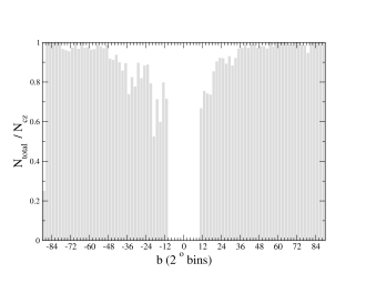
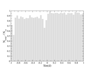
Figure 1.— Left: 2MASS redshift completeness is plotted as a function of galactic latitude. The high latitude regions are very complete, except for $b\backsim-90^{\circ}$ values where the observed low value is due to a very small number of total galaxies. As $b\rightarrow 0^{\circ}$ there is a decrease in the fraction of measured redshifts due to the difficulty of obtaining redshifts close to the galactic plane. The area $|b|<10^{\circ}$ is excluded. Right: Redshift completeness in equal area bins of declination for sin$|b|\geq 0.2$. Note the higher incompleteness in the southern equatorial hemisphere.

Fig. 1 shows the 2MASS redshift completeness percentages in terms of the galactic latitude and declination (D). While the redshifts are highly complete at high Galactic latitudes, there is a decline in the completeness at lower $|b|$. In the Northern celestial hemisphere, the completeness is very high, but drops in the southern hemisphere. We also find that the redshift incompleteness is not correlated to the magnitude.

Since the overall completeness is high, and hence the corrections are small, we model the incompleteness with a simple functional form. We assume that the probability of observing a galaxy in our sample with a redshift is a separable function $P_{cz}(b$,D)$=P_{1}(b)P_{2}$(D).

Fig 1 shows a completeness is $\sim 1$ at high Galactic latitudes, with a decrease completeness towards the Galactic plane. After trial and error, for $P_{1}(b)$ we adopt the functional form

$$P_{1}(b\geq 11.5^{\circ}) = 1-\exp\left[-\frac{\sin b}{\sin b_{\mathrm{N}}}\right]$$

$$P_{1}(b\leq-11.5^{\circ}) = 1-\exp\left[-\frac{\sin b}{\sin b_{\mathrm{S}}}\right]$$ (4)

For declination, the northern hemisphere is quite complete whereas the southern hemisphere is less so. Fig, 1 shows no strong dependence on declination within a given hemisphere, so we have chosen to simply fit with a step function

$$P_{2}(\mathrm{D}\geq 0) = \mathrm{D}_{\mathrm{N}}\equiv{1}$$

$$P_{2}(\mathrm{D}\leq 0) = \mathrm{D}_{\mathrm{S}}$$ (5)

The likelihood of the given set of galaxies with and without redshift is

$${\cal{L}}_{cz}=\prod_{i=1}^{N_{cz}}P_{1}(b_{i})P_{2}(\mathrm{D}_{i})\times\prod_{i=1}^{N_{\mathrm{miss}}}1-[P_{1}(b_{i})P_{2}(\mathrm{D}_{i})]$$ (6)

where the first product sum is over galaxies with measured redshift and the second is over those having been detected with no associated redshift.

The maximum likelihood solution yields best fit parameters $b_{\mathrm{N}}=8.33^{\circ}$ and $b_{\mathrm{S}}=-11.9^{\circ}$, and D${}_{\mathrm{N}}\equiv 1$ and D${}_{\mathrm{S}}=0.933$. We correct for incompleteness in $b$ and declination by weighting the galaxies with redshifts by $1/[P_{1}(b)\,P_{2}$(D)].

2.1.2 Cloning the Zone of Avoidance

Due to increasing redshift incompleteness at low galactic latitudes, only galaxies satisfying $|b|\geq 11.5^{\circ}$ were selected. Leaving the unsurveyed regions empty would cause systematic errors in the dynamical model, because this region would behave as a void. This would have the effect of creating a false outflow, as can be understood through the $\delta$ term in Equation (1).

There are several ways in which this effect can be corrected. For instance, the volume can be filled with a uniform distribution of galaxies that exactly match the surveys’ average density. This method has the benefit of alleviating the systematic errors associated with the empty space, and since $\delta=0$ in this region, there is no gravitational effect.

We chose instead to fill the plane by interpolating or cloning adjacent, equal area regions above and below the galactic equator (Hudson 1993). Due to the infrared nature of the survey, a galactic latitude cut as low as $|b|=11.5^{\circ}$ could be made, which meant only a relatively small strip had to be cloned, as opposed to optical surveys which typically have higher limiting $|b|$ (Santiago et al. 1995; Giuricin et al. 2000). Hudson (1994) found that if uniform density was assumed then the values of $\beta$ are only $\sim 10\%$ higher. However, surveys in the ZoA (Staveley-Smith et al. 2000) suggest that cloning is a better approximation.

In our cloning procedure, the $K_{20}$ apparent magnitude and redshift, along with all of the other associated properties of a cloned galaxy remain the same as the parent, with the exception of a new galactic latitude which depends on the parent and cutoff galactic latitudes through, $\sin{b_{\mbox{\footnotesize clone}}}=\sin{b_{\mbox{\footnotesize parent}}}-\sin{b_{\mathrm{min}}}$.

2.2. Luminosity Function: $\Phi\left(L\right)$

In order to correct for galaxy incompleteness due to the imposed flux limit, it is necessary to know the luminosity function (hereafter LF). The empirical LF is often fitted by an analytical expression first described by Schechter (1976),

$$\Phi\left(L\right)dL=\phi^{*}\left(\frac{L}{L^{*}}\right)^{\alpha}\exp\left[-\frac{L}{L^{*}}\right]\frac{dL}{L^{*}}$$ (7)

in which $L^{*}$ (or equivalently $M^{*}$ if we describe it in terms of absolute magnitudes) is the fiducial magnitude and represents the point in which the LF changes from a power law (with slope $\alpha$) to an exponential.

To estimate the LF parameters, we adopt the density-independent method of Sandage et al. (1979). In Section 2.3.3 below, we will outline the redshift transformation method which uses the smoothed, weighted density field to make iterative corrections to the distance of each galaxy based on an assumed $\beta$. After each iteration, when the distances to every galaxy have been updated, we recalculate the LF parameters. Thus in contrast to, for example, deep samples in which redshift is used as a proxy for distance, in our case a self-consistent set of LF parameters for each value of $\beta$ is derived. Nevertheless, at low redshifts the uncertainty in a galaxy’s distance due to its peculiar velocity is large, so we have used only galaxies in the distance range $1500$ km s^-1 to $6500$ km s^-1 to estimate the LF parameters, and excluded faint galaxies with $M_{K_{20}}>-18$.

We obtain best fitting values $M^{*}_{K_{20}}=-23.42$, $\alpha=-0.982$ and $\phi^{*}_{K_{20}}=0.011$ (in $h^{3}$Mpc^-3) from the analysis of the real space galaxy distribution (at the best fitting $\beta$, see Section 3.3). This is in agreement with the results of Cole et al. (2001) who used the 2MASS and 2dF galaxy redshift surveys to derive values for the parameters $M^{*}_{K_{20}}-5$log${h}$ , $\alpha$ and $\phi^{*}_{K_{20}}$ in the $K_{s}$ band yielding, $-23.44\pm 0.03$, $-0.96\pm 0.05$ and $0.0108\pm 0.0016h^{3}$ Mpc^-1 respectively. The likelihood analysis of the LF was performed with and without the inclusion of cloned galaxies. We find that there is no appreciable difference in either case, as expected since the Sandage et al. method is density-independent. In Section 4 we explore how morphology affects the LF parameters by segregating the density field into early and late-types.

2.3. Transforming Redshifts to Real Space Distances

2.3.1 Weighting the Sample

Knowing the LF and completeness of the sample, we can calculate the selection function (the probability that a galaxy is included in the redshift sample) at any distance $r$ as,

$$\phi\left(r\right) \equiv \frac{\int_{4\pi r^{2}f_{\min}}^{\infty}\Phi\left(L\right)dL}{\int_{L_{\mathrm{min}}}^{\infty}\Phi\left(L\right)dL}\qquad r\geq r_{\mathrm{min}}$$

$$\equiv 1\qquad\qquad\qquad\qquad\;\;r<r_{\mathrm{min}}$$

where $f_{\mathrm{min}}$ is the flux corresponding to $K_{\mathrm{20,lim}}=10.5$. In practice the luminosity function is poorly constrained at the faint end, and hence we place a lower limit on the integral at $L_{\mathrm{min}}=4\pi r_{\mathrm{min}}^{2}f_{\mathrm{min}}$. $L_{\mathrm{min}}$ corresponds to $M_{K}=K_{\mathrm{20,lim}}-5\log(r_{\mathrm{min}}/10\mathrm{pc})$, which is $-18$ for $r_{\mathrm{min}}=5h^{-1}$ Mpc.

We assign extra weight, $1/\phi(r)$, to galaxies with measured redshifts to account for the galaxies in the same volume that were not detected or failed to meet the selection criteria. This is equivalent to adding galaxies at every position where we have a galaxy with a measured redshift.

Weights are assigned to all galaxies in our sample limit, $r\leq R_{\mathrm{max}}$. Galaxies outside of $R_{\mathrm{max}}$ are set to a weight of zero. The sum of the weights divided by the volume within $R_{\mathrm{max}}$ yields the average number density.

2.3.2 Smoothing the Sample

The galaxy distribution obtained from redshift surveys is a point process. If we were to apply linear theory directly, the predictions would diverge near the weighted points. We smooth the density field so that the velocity field is continuous and so that linear theory applies. This is accomplished by applying the following equation to the density field,

$$\delta\left(\mathbf{r}\right)=\frac{\rho\left(\mathbf{r}\right)-\overline{\rho}}{\overline{\rho}}=\frac{1}{\overline{n}}\sum_{i}^{N_{\mathrm{gal}}}\frac{1}{\phi(r_{i})}\left[W\left(\frac{\left|\mathbf{r-r}_{i}\right|}{r_{\mathrm{sm}}}\right)-1\right]$$ (9)

in which $W$ is a smoothing kernel and $\overline{n}$ is the number density of the $N_{\mathrm{gal}}$ weighted objects. We have chosen to use a top-hat kernel in which $W=|\mathbf{r}-\mathbf{r}_{i}|^{3}/r_{\mathrm{sm}}^{3}$ for $\left|\mathbf{r}-\mathbf{r}_{i}\right|<r_{\mathrm{sm}}$ and set to unity otherwise. We use a fixed smoothing length $r_{\mathrm{sm}}$ of $500$ km s^-1 independent of distance.

2.3.3 Reconstruction Procedure

We now discuss the reconstruction method used to transform the measured redshifts into real space distances, $r$, for the model. Given a smoothed all sky density field, the peculiar velocity of any galaxy can be estimated via Equation (2), and used to make distance corrections to the sample. We follow a similar method to that of Yahil et al. (1991) who use an iterative technique in which gravity is adiabatically “turned on” by increasing $\beta$. The following outlines a recipe for a self-consistent solution to real space density and velocity maps given only positions and redshifts.

Prior to the start of the iterative procedure, we collapse the so-called “Fingers of God” (nonlinear redshifts distortions resulting in an apparent radial stretching along the line of sight) by placing all grouped galaxies at a common median redshift, $cz_{\mathrm{LG}}$, and angular position.

Initially, galaxies are assigned distances that are equal to their Local-Group-frame redshifts. A value of $\beta$ is defined at each step of the iteration and the resulting peculiar velocity field is calculated. We perform 100 steps, defining a density and velocity field at each iteration from $\beta=0.01$ to $\beta=1.00$ in steps of $0.01$. At each iteration the following steps are performed.

1. The likelihood function for the LF is minimized to determine the best fit parameters and a number weight is assigned to each galaxy according to its distance as described in Section 2.3.1.

2. Galaxies are cloned to fill the void as described in Section 2.1.2, assigning each cloned galaxy the properties of its parent, including its weight.

3. The average density $\overline{n}$ of all galaxies within $R_{\mathrm{max}}$ is calculated. This then defines the density contrasts $\delta_{\mathrm{g}}$.

4. A peculiar velocity is calculated for each galaxy using Equation (2). We average the current peculiar velocity with that of the past 5 iterations. As we step through $\beta$, we are essentially turning on the gravity, and since increases in $\beta$ are very small at each step, changes in weight and positions are also small over this range. The averaging has the benefit of damping out any unphysical oscillatory behavior

   With this information we update the distance of each galaxy according to the equation for total recession velocity, $r_{i}=cz_{\mathrm{LG,i}}-u(r_{i})$ (where $i$ denotes the $i^{th}$ of $N_{\mathrm{gal}}$ galaxies). Note that the distance to each galaxy in the sample changes at each iteration. In particular, after an iteration, a galaxy’s distance may “move” it across $R_{\mathrm{max}}$. Therefore, at each iteration, we update the positions of all galaxies with $cz_{\mathrm{\mathrm{L}G}}<9000$ km s^-1, which is well beyond $R_{\mathrm{max}}$. A galaxy residing in the region $r>R_{\mathrm{max}}$ and $cz_{\mathrm{L}G}<9000$ km s^-1 is assigned a weight of zero, and therefore contributes nothing to the density and predicted peculiar velocity fields. If a subsequent iteration brings it within $R_{\mathrm{max}}$, it is assigned a weight. Similarly, if an iteration brings a galaxy from $r<R_{\mathrm{max}}$ to $r>R_{\mathrm{max}}$ it is assigned a weight of zero. In this way, we maintain a density field based on a self-consistent distance limit $R_{\mathrm{max}}$.

We repeat the above steps at each iteration. Thus after the iterative procedure is complete, we have 100 density and velocity fields (specified by $\beta$), each of which can be compared to measured peculiar velocity data.

2.3.4 Cosmography

Figure 2.— The isodensity contours for a slice through the Supergalactic Plane of the reconstructed 2MASS density field. The density field has been smoothed with a Gaussian kernel of $500$ km s^-1. The heavy contour indicates mean density, $\delta_{\mathrm{g}}=0$, and increases in steps of $\Delta\delta_{\mathrm{g}}=0.5$. It can be seen that the zone of avoidance has been filled with cloned galaxies. Superimposed is the predicted peculiar velocity field for $\beta_{K}=0.49$.

Fig. 2 shows the Supergalactic Plane maps of the reconstructed density field and the resulting velocity field for our best fit $\beta_{K}=0.49$ as derived using the 2MASS redshift data. The galaxy density field is smoothed using a Gaussian kernel with a smoothing radius of $500$ km s^-1.

The plot shows the major structures that are located in the Supergalactic SGX-SGY Plane as well as the resulting flow fields. Directly above the center (LG) in the positive SGY direction is the Virgo Supercluster, with an associated peak overdensity of $\delta_{\mathrm{g}}=2.7$. At $SGX=-4000$ to $-3000$ km s^-1 and $SGY=1000$ to $2500$ km s^-1 is the Great Attractor (GA). The peak in seen in Fig. 2 is coincident with the cluster Abell 3574 ($r\sim 5300;\delta_{\mathrm{g}}=3.4$), but the highest peak in this region lies slightly off the Supergalactic Plane, and is coincident with the Centaurus cluster at ($r\sim 3600$ km s^-1; $\delta_{\mathrm{g}}=4.7$) with a secondary peak at Pavo II (Abell S0805; $r\sim 4500$ km s^-1; $\delta_{\mathrm{g}}=4.6$). Note that what may be the most massive cluster in the GA region, Abell 3627 (Kraan-Korteweg et al. 1996) is not in our sample because of its low Galactic latitude ($b=-7^{\circ}$). However, the dynamical influence of a single cluster, even a massive one such as Abell 3627, is small. Instead the peculiar velocity field is more strongly affected by the large-scale overdensity of the supercluster as a whole. It is these large-scale overdensities that are crudely reproduced by our cloning procedure.

The Perseus-Pisces (PP) supercluster shows the largest overdensity of $\delta_{\mathrm{g}}=5.5$, coincident with the Perseus cluster, located near the sample limit and at the edge of the ZoA, in the SGX, -SGY direction. Note however that the overdensity may be enhanced due to the cloning of Perseus. The region at $SGX=2200$ km s^-1 and $SGY=-5000$ km s^-1 is harder to classify. It has an overdensity of $\delta_{\mathrm{g}}=2.6$, and appears to coincide with Abell 168A/Abell 1194 overdensities. The Coma cluster lies outside of our sampled distance limit at around a redshift of $cz=7000$ km s^-1. In contrast, the -SGX, -SGY quadrant is almost completely devoid of overdensities, and is dominated by the Sculptor void which exhibits a weak velocity outflow.

3. Velocity-Velocity Comparisons

With the full velocity field modelled, we now make comparisons to peculiar velocity data sets. Below is a discussion of the properties of the peculiar velocity sets used, as well as the methods used in their comparison to the model.

3.1. Peculiar Velocity Data

We compare our predictions to three published peculiar velocity data sets. Each of which vary in sample size and typical distance errors and method of obtaining the secondary distance information.

Our subsample of the Spiral Field I-Band (hereafter SFI; Haynes et al 1999a,b) survey consists of 836 galaxies of morphological type Sbc-Sc, in which distances have been derived from the I-Band Tully-Fisher relation over the full sky. Typical distance errors are on the order of 20% for our subsample, which extends to $5000$ km s^-1. The characteristic depth of the sample, which is the weighted distance from which which the majority of the signal arises is

$$d_{c}=\frac{\sum d_{i}w_{i}}{\sum w_{i}}$$ (10)

where the weights $w_{i}=1/\sigma_{d,i}$ and $\sigma_{d,i}$ is the distance error. For the SFI set, $d_{c}=2700$ km s^-1, so the characteristic distance error is $\sigma_{d_{c}}=540$ km s^-1.

The I-band Surface Brightness Fluctuation (SBF, Tonry et al. 2001) survey consists of 266 galaxies extending to a distance of  $4000$ km s^-1. The uncertainties in the distance estimates varies inversely with the resolution of the images. Typical distance errors for our sample are of the order of 8%, approximately half that of SFI. The characteristic depth is 1200 km s^-1 having $\sigma_{r_{c}}=96$ km s^-1.

The final data set is a compilation of supernovae of type Ia (SN Ia, Tonry et al. 2003) and consists of 59 SNe extending to a distance of $6000$ km s^-1, with typical errors of 8%. The characteristic depth of this sample is 2200 km s^-1 with $\sigma_{r_{c}}=176$ km s^-1.

3.2. Method

We apply two v-v comparison methods. Our primary method is a slight variant of the VELMOD method. For comparison, we also apply a simple and complementary $\chi^{2}$ fitting method.

3.2.1 VELMOD

The procedure outlined here differs slightly from the VELMOD method by Willick et al. (98). Our procedure uses two free parameters: $\beta$, which scales the predicted peculiar velocities, and $H_{0}$, which allows for a rescaling of the published distances. In contrast, Willick et al. fit $\beta$ as well as the parameters of the TF relation.

Specifically, we maximize the probability of each galaxy having its observed velocity, $P\left(cz_{\mathrm{obs}}\right)$. We construct the joint probability distribution of redshift and the (unobservable) true distance,

$$P\left(cz_{\mathrm{obs}},r\right)=P\left(cz_{\mathrm{obs}}|r\right)P\left(r\right)$$ (11)

where the first term

$$P\left(cz_{\mathrm{obs}}|r\right)=\frac{1}{\sqrt{2\pi}\sigma_{v}}\exp\left[-\frac{\left[cz_{\mathrm{obs}}-\left(H_{0}r+\beta u\left(r\right)\right)\right]^{2}}{2\sigma_{v}^{2}}\right]$$ (12)

is a description of the redshift-distance relation in terms of a Gaussian probability distribution. The predicted $cz_{\mathrm{pred}}$ has three parts; an expansion velocity; a part due to the linear perturbations of the surrounding overdensities, $u(r)$, and a part which is often referred to as velocity noise, $\sigma_{v}$, assumed to be Gaussian, arising from strongly non-linear processes. For this calculation, $\sigma_{v}$ is fixed at $200$ km s^-1 for field galaxies. This allows for uncertainties in the linear predictions, nonlinear motions and observational errors in $cz_{\mathrm{obs}}$. This value of $\sigma_{v}$ is chosen because it gives reasonable reduced $\chi^{2}$ fits (see Section 3.2.2), although our recovered values of $\beta$ are not sensitive to precise value chosen for $\sigma_{v}$. An additional velocity error was added in quadrature to $\sigma_{v}$ to account for extra velocity dispersion for galaxies associated with clusters: $\sigma_{\mathrm{cl}}=\sigma_{0}/\sqrt{1+(r/r_{0})^{2}}$, where $\sigma_{0}=700(400)$ km s^-1 and $r_{0}=2(1)$ Mpc are adopted for Virgo (Fornax) respectively (Blakeslee et al. 1999).

The second term in eq. 11 is the a priori probability of observing an object at distance $r$

$$P\left(r\right)\propto\exp\left[-\frac{\left(r-d\right)^{2}}{2\sigma_{d}^{2}}\right]\left(1+\delta_{\mathrm{g}}\right)$$ (13)

and is a Gaussian with mean equal to the estimated secondary distance $d$ with an additional term $(1+\delta_{\mathrm{g}})$, proportional to the number density of galaxies, to account for inhomogeneous Malmquist bias. The $(1+\delta_{\mathrm{g}})$ term is evaluated using the 2MASS density field, smoothed with a Gaussian filter of $500$ km s^-1. In principle, for each peculiar velocity dataset, one should use $\delta_{\mathrm{g}}$ for the appropriate morphological type, for example, $\delta_{\mathrm{E}}$ for the SBF dataset. In practice, as we will discuss in Section 5, the correction arising from the $(1+\delta_{\mathrm{g}})$ term is small except for the SFI case. In Section 4 we show that the bias $b$ for Spiral and later types appears to be very similar to that of the sample as a whole, thus justifying the simpler approach adopted here.

The expression $P(cz_{\mathrm{obs}})$ can be obtained by integrating over all possible distances,

$$P\left(cz_{\mathrm{obs}}\right)=\int_{0}^{\infty}P\left(cz_{\mathrm{obs}}|r\right)P\left(r\right)dr\,.$$ (14)

Equation (14) is then normalized over all possible velocities.

The VELMOD method then maximizes the log likelihood, $\sum_{i}\ln[P(cz_{i})]$, over all galaxies in the peculiar velocity data set as a function of the free parameters $\beta$ and $H_{0}$.

3.2.2 $\chi^{2}$ method

In addition to VELMOD, we perform a simple $\chi^{2}$ minimization. The $\chi^{2}$ function is constructed from the differences between the observed $cz_{\mathrm{obs}}$ and that which is predicted from a combination of our radial velocity and the galaxies measured distance. We minimize the function,

$$\chi^{2}=\sum\frac{[cz_{\mathrm{obs}}-(H_{0}d+\beta u(d))]^{2}}{\sigma_{cz}^{2}}$$ (15)

which is similar to that contained inside the parenthesis of Equation (12). In this case however we do not evaluate $u(r)$ at all possible values of $r$ and marginalize, but instead use the peculiar velocity at the estimated distance $d$. To the extent that the peculiar velocity predictions do not change rapidly on the scale of the distance error, $\sigma_{r}$, this approximation will be accurate. The error $\sigma_{cz}=\sqrt{{\sigma_{v}}^{2}+{\sigma_{d}}^{2}}$, where $\sigma_{v}$ is the same as in Equation (12). Note that this application of the $\chi^{2}$ method neglects inhomogeneous Malmquist bias. Although it is possible to correct for the estimated distances for this bias (Hudson 1994a), we have not done so in this paper.

3.3. Results

The VELMOD analysis applied to the SN Ia, SBF and SFI peculiar velocity sets yields the likelihood confidence ellipses shown in Fig. 3. Table 1 summarizes the results for the peculiar velocity comparisons with those predicted by the reconstructed 2MASS density field. $\beta_{\mathrm{VELMOD}}$ indicates the value obtained from the first moment of the marginalized $\beta$ probability distribution function (PDF) obtained from the VELMOD analysis. The $\beta_{\mathrm{VELMOD}}$ values are then combined to determine the best fitting $\beta=0.49\pm 0.04$, which is indicated as All in the last row of Table 1. The $\beta_{\chi^{2}}$ values are quoted for the $\chi^{2}$ minimization. There was only one free parameter in the $\chi^{2}$ fits corresponding to $\beta$, and $H_{0}$ was held constant at the best fit VELMOD value. Since there is only one free parameter in the fits, the number of degrees of freedom (DOF) is $N_{\mathrm{gal}}-1$.

Table 1Summary of $\beta$ determinations: VELMOD and $\chi^{2}$ minimization results.

Set:	$\beta_{\mathrm{VELMOD}}$	$\beta_{\chi^{2}}$	D.O.F	$\chi^{2}$
SN Ia	$0.47\pm 0.06$	$0.45\pm^{+0.09}_{-0.05}$	$59$	$42$
SBF	$0.46\pm 0.06$	$0.44\pm^{+0.05}_{-0.07}$	$266$	$238$
SFI	$0.55\pm 0.05$	$0.53\pm^{+0.04}_{-0.03}$	$831$	$756$
All	$0.49\pm 0.04$	$-$	$-$	$-$

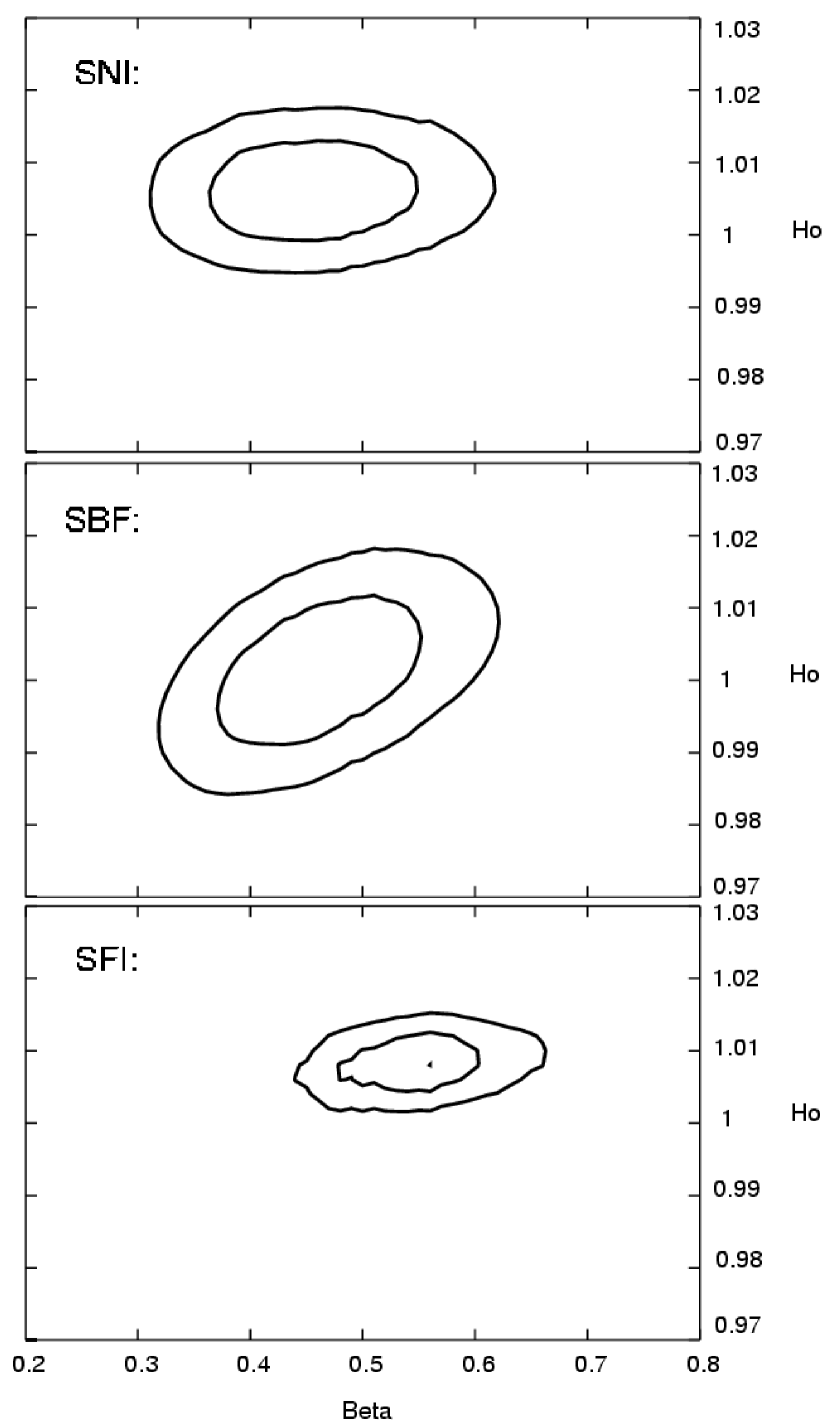
Figure 3.— The $68\%$ and $90\%$ joint probability contours on $\beta$ and $H_{0}$ are plotted for the VELMOD likelihood analysis for each peculiar velocity data set (SN Ia, SBF, SFI) and the derived 2MASS velocity field. Note that $H_{0}$ is very close to unity in all cases. This joint distribution is then marginalized (over $H_{0}$) to obtain a probability distribution function for $\beta$.

With the adopted value of $\sigma_{v}$, the $\chi^{2}$ values are reasonable. The agreement between the SN Ia and the SBF samples is evident, and these two samples agree (within errors) with the slightly higher $\beta$ determination for the SFI sample. All peculiar velocity datasets agree within the determined errors. The agreement is reinforced in Fig. 4, where we plot the measured SN Ia, SBF and SFI peculiar velocities against those predicted by 2MASS for each respective $\beta_{\mathrm{VELMOD}}$.

Figure 4.— Comparisons of SN Ia, SBF and SFI peculiar velocities to those which have been derived from the 2MASS modelled velocity field out to a distance of $6500$ km $s^{-1}$. Errors are defined by $\sigma_{cz}$, but for SFI and SBF data only one in three error bars are plotted. Predictions are scaled to $\beta=1$, so the slope of best fit corresponds to the value of $\beta$. The solid line indicates the best fit to the individual data set shown, and the dotted line is the global fit ($\beta=0.49$).

4. Effect of Morphology

It is likely that mass is related to light in a way more complicated than suggested by linear biasing. While such deviations may be small on linear scales probed by peculiar velocities, there remains the possibility of measuring such deviations. In particular, it is well-known that early-type galaxies are preferentially found in dense environments. In the case of a toy model in which, for example, all mass of the Universe was in clusters, with no mass in the field, then one would expect the elliptical density field to be a better predictor of peculiar velocities than that of spirals. So it is of interest to explore the predictions of density fields pre-selected by morphological type.

We have morphological types for nearly $97\%$ of our sample. We consider two subsamples, an early-type (E+S0) sample having $T\leq 0$, and a late-type (S+Irr) sample having $T>0$. Here T represents a numerical code for the revised (de Vaucouleurs) morphological type. Our cloned sample contains $N_{\mathrm{E+S0}}=2486$ galaxies. Despite the $K_{s}$-band selection, the 2MASS redshift survey contains more late-type galaxies than early-types, such that $N_{\mathrm{S}}=3795$.

We analyzed both in the same manner as outlined in Section 2.3.3. The LF parameters for the early-type galaxies are $M^{*}_{K_{20}}=-23.57$ and $\alpha=-0.72$ and the corresponding values for the late-types are $M^{*}_{K_{20}}=-23.08$ and $\alpha=-0.79$. Note that both of these are flatter than the full density field, which may be a result of incompleteness in morphological types at the faint end. This trend is also observed in the recent determination of early and late-type LF’s by Kochanek et al. (2001). They find $M^{*}_{K_{20}}=-23.53\pm 0.06$ and $\alpha=-0.92\pm 0.10$ and $M^{*}_{K_{20}}=-22.98\pm 0.06$ and $\alpha=-0.87\pm 0.09$ for the early and late-type LF parameters respectively. They used $7\leq K_{20}\leq 11.25$ mag, with $cz>2000$km s^-1 and a limiting latitude of $|b|\geq 20^{\circ}$ for an approximately equal sample size.

Figure 5.— The reconstructed E+S0 (left) and S+Irr (right) density and velocity fields. Contours are as in Fig.2. Predicted peculiar velocities are for the best fit values from Table 2. While general features are consistent in both fields, the relative contrast indicates that the early-type galaxies are more clustered.

The derived density and velocity fields from the two morphological subsamples are shown in Fig. 5. The most distinct difference between the fields is that the early-types clearly reside in higher density regions. The density contrast is more significant in every clustered region, as is indicated by the increase in contour line density. Since the amount of clustering is quantified through the biasing parameter $b$, we can also measure $b$ via the $\beta$ of best fit to the peculiar velocities.

Table 2 $\beta$ dependency on morphology.

Set:	$\beta_{\mathrm{VELMOD}}$	$\beta_{\chi^{2}}$	D.O.F	$\chi^{2}$
		Late-Type (Spirals)
SN Ia	$0.46\pm^{+0.06}_{-0.07}$	$0.48\pm^{+0.05}_{-0.07}$	$58$	$46$
SBF	$0.45\pm 0.06$	$0.38\pm^{+0.06}_{-0.04}$	$265$	$244$
SFI	$0.50\pm^{+0.04}_{-0.05}$	$0.48\pm^{+0.02}_{-0.03}$	$830$	$770$
All	$0.48\pm 0.04$	$-$	$-$	$-$
		Early-Type (E+S0)
SN Ia	$0.32\pm 0.05$	$0.35\pm^{+0.05}_{-0.04}$	$58$	$40$
SBF	$0.28\pm 0.04$	$0.25\pm^{+0.03}_{-0.02}$	$265$	$241$
SFI	$0.30\pm 0.04$	$0.33\pm^{+0.02}_{-0.03}$	$830$	$784$
All	$0.30\pm 0.03$	$-$	$-$	$-$

The results of the VELMOD and $\chi^{2}$ minimizations for the morphological subsamples are given in Table 2. For the VELMOD determinations there is excellent agreement between the values of $\beta$ derived from each of the peculiar velocity data sets for both early- and late-type density fields. There is also good agreement between the $\chi^{2}$ and VELMOD techniques. The early-type density field yields $\beta$ values ($\sim 0.3$) that are consistently lower than in the late-type case ($\sim 0.48$). This suggests that the early-type density field is more strongly clustered $\beta_{\mathrm{S}}/\beta_{\mathrm{E}}=b_{\mathrm{E}}/b_{\mathrm{S}}\sim 1.6$ in the $K_{s}$-band.

In principle, it is possible to test whether early- or late-types are better tracers of the mass by comparing the quality of the fit from the two different density fields to the same peculiar velocity sample. For the SN Ia and SBF data sets, the peculiar velocity field predicted by early-types has a lower $\chi^{2}$ value, although this difference is only significant for the SN Ia sample. For the SFI data set, the opposite is true: the late-type density field yields a better goodness-of-fit. One might be concerned that, because the early-type density field is sparser (and hence more subject to shot noise), its predicted peculiar velocities are noisier and hence the $\chi^{2}$ may be biased high. However, the early-type galaxies are also more strongly clustered, with the result is that the signal-to-noise ratios of the density fields are similar. To put it another way, the higher degree of noise in the density field is suppressed by the lower value of $\beta$. We have performed tests to simulate the effects of sparse sampling on the goodness-of-fit statistic $\chi^{2}$, and find no conclusive evidence for a difference between early and late-type density fields. However, further tests are required to understand the systematics in greater detail.

5. Discussion

5.1. Potential Systematic Effects

We now discuss the potential systematics which might affect our results. These include smoothing, external gravity contributions, sparseness of the sample, as well as the possibility of inhomogeneous Malmquist bias.

Berlind at al. (2001) explored the effects of applying various biasing schemes and smoothing lengths in the determination of $\beta$. For the case of linear biasing, they find that the optimal smoothing length is roughly a $3h^{-1}$Mpc Gaussian sphere, which is close to our adopted $5$ $h^{-1}$Mpc top-hat smoothing. In contrast, for example, had we adopted a top-hat smoothing of $8h^{-1}$Mpc, the results of Berlind et al. suggest that our derived value of $\beta$ would have been biased too high by $\sim 10\%$. Therefore our choice of smoothing length is close to optimal and we do not expect a significant bias in our determination of $\beta$.

The external velocity field can be reasonably described by the two main components (a dipole and a quadrupole, i.e. bulk and shear). Since the analysis was carried out in the LG frame, we need not worry about any external dipole contributions, however, this is not true for any higher order contributions, such as the quadrupole, that may exist. Willick & Strauss (1998) suggested the existence of a residual quadrupole velocity field that was not well modelled by the IRAS 1.2Jy gravity field. We find no evidence of a residual quadrupole in the SN Ia and SFI data. The SBF data suggests a marginally significant quadrupole, but the inclusion of such a term does not significantly affect the value of $\beta$.

Another possible systematic effect is related to the discreteness of the density fields used to make our velocity predictions. Since the galaxy density field is a sparsely sampled, this can lead to shot noise in the velocity predictions. To test whether the sample size affects the determination of $\beta$, we generated a sparse-sampled density field comprising of $50\%$ of the full 2MASS density field. For this test, we find a small change ($\sim 2-3\%$) in the predicted value of $\beta$, which is negligible compared to the random errors on $\beta$.

Finally, let us discuss the corrections made for inhomogeneous Malmquist bias (IMB), which is a Malmquist bias arising from distance errors scattering peculiar velocity data away from overdensities. Since their redshifts are not scattered significantly, the resulting pattern mimics infall, leading to a biased estimate of $\beta$. The strength of the bias increases as the square of the typical peculiar velocity error, $\sigma_{d_{c}}$, thus we expect the SFI sample to be most affected by the IMB. The VELMOD technique includes a $(1+\delta_{\mathrm{g}})$ correction to the distance probability function $P(r)$ which corrects for this effect. It is nevertheless of interest to estimate the effect of the IMB on different samples, which can be done by repeating the analysis omitting the $(1+\delta_{\mathrm{g}}$) term. For the SN Ia and SBF samples, the correction is negligibly small (0.02) in $\beta$. The SFI data set is more sensitive to IMB; our result for this sample $\beta=0.55$ (with IMB correction) would have been $\beta=0.71$ without the IMB correction. For deeper samples with large errors, it is clearly important to account for IMB.

In summary, we have not identified any systematics which affect the result at a level greater than the random errors.

5.2. Comparison with Other Results

This paper is the first comparison between the 2MASS density field and peculiar velocity surveys. However, our results are consistent with previous analyses comparing the 2MASS dipole to the motion of the LG. Maller et al. (2003) assumed $\Omega_{\mathrm{m}}=0.27$ and found $b_{K}=1.06\pm 0.17$ which is equivalent to $\beta_{K}=0.48\pm 0.08$. Our result is also consistent with the upper limit $\beta_{K}<0.55\pm 0.2$ derived by Erdogdu et al. (2005).

Table 3A summary of the $\beta$ results from this paper and recent v-v determinations obtained from the literature

Comparison Sets	$\beta$	$\left(\frac{\Omega_{\mathrm{m}}}{0.3}\right)^{0.6}\sigma_{8}$	Reference
SN Ia $vs.$ 2MASS	$0.47\pm 0.06$	$0.86\pm 0.15$	This Study
SBF $vs.$ 2MASS	$0.46\pm 0.06$	$0.84\pm 0.15$	This Study
SFI $vs.$ 2MASS	$0.55\pm 0.05$	$1.02\pm 0.15$	This Study
SN Ia+SBF+SFI $vs.$ 2MASS	$\bf 0.49\pm 0.04$	$\bf 0.91\pm 0.12$	This Study
Mark III $vs.$ IRAS 1.2 Jy	$0.50\pm 0.10$	$0.82\pm 0.16$	Davis et al. (1996)
SN Ia $vs.$ IRAS 1.2 Jy	$0.40\pm 0.15$	$0.65\pm 0.25$	Riess et al. (1997)
SBF $vs.$ IRAS 1.2 Jy	$0.42^{+0.10}_{-0.06}$	$0.70\pm^{+0.16}_{-0.10}$	Blakeslee et al. (1999)
SFI $vs.$ IRAS 1.2 Jy	$0.60\pm 0.10$	$0.99\pm 0.09$	da Costa et al. (1998)
Mark III $vs.$ IRAS 1.2 Jy	$0.50\pm 0.04$	$0.82\pm 0.08$	Willick & Strauss (1998)
Mark III $vs.$ PSCz	$0.60\pm 0.10$	$0.99\pm 0.19$	Saunders et al. (1999)
ENEAR $vs.$ PSCz	$0.50\pm 0.10$	$0.82\pm 0.16$	Nusser et al. (2001)
SN Ia $vs.$ PSCz	$0.54\pm 0.06$	$0.89\pm 0.10$	Radburn-Smith et al. (2004)
SFI $vs.$ PSCz	$0.42\pm 0.04$	$0.66\pm 0.08$	Branchini et al. (2001)
SEcat $vs.$ PSCz	$0.51\pm 0.06$	$0.84\pm 0.10$	Zaroubi et al. (2002)
Weighted IRAS Avg.	$\bf 0.50\pm 0.02$	$\bf 0.83\pm 0.06$	-
2MASS and IRAS Avg.		$\bf 0.85\pm 0.05$	-

Table 3 lists our results and recent $\beta$ measurements obtained via velocity-velocity methods obtained using the IRAS 1.2 Jy and PSCz surveys. The 2MASS $\beta$ values agree quite well with IRAS values. However, when comparing the 2MASS predictions of $\beta$ to the IRAS values, one should keep in mind that the IRAS samples are dominated by late-type galaxies. Consequently, the strength of the clustering, or bias, is likely to differ and the comparisons of $\beta$ may not be straight forward. With this in mind, it is preferable to transform the results into a form that is independent of the details of the density field used. This can be accomplished by noting that the linear biasing factor $b$ relates the r.m.s. galaxy fluctuations, $\sigma_{\mathrm{8,g}}$, to the amplitude of r.m.s. mass fluctuations, $\sigma_{8}$, where the subscript 8 indicates that the density fluctuations have been averaged in top-hat spheres of radius $8$ $h^{-1}$Mpc. If $\sigma_{\mathrm{8,g}}$ is known, we may express our results as $\beta_{\mathrm{g}}\sigma_{\mathrm{8,g}}=\Omega_{\mathrm{m}}^{0.6}\sigma_{8}$.

From the 2MASS $K_{s}$ band density field reconstructed in this paper, we have measured directly the r.m.s fluctuations in 8 $h^{-1}$ Mpc spheres. Allowing for shot noise, we find a value of $\sigma_{8,K}=0.90$ (in reconstructed “real” space). We have not measured the uncertainty in this quantity, but note that this result is consistent with $\sigma_{8,K}=1.0\pm 0.1$ found by Maller et al. (2005) for a larger $K_{s}$ band 2MASS sample, although it is lower than the value found by Frith et al. (2005): $1.16\pm 0.04$. Luminosity-dependent biasing may account for some of the difference between these results. Here we adopt $\sigma_{8,K}=0.9\pm 0.1$ to obtain the result $\sigma_{8}(\Omega_{\mathrm{m}}/0.3)^{0.6}=0.91\pm 0.12$. We note that the is dominant contribution to the uncertainty is from the uncertainty in $\sigma_{8,K}$. We expect that $\sigma_{8,K}$ will be better determined in the near future from the 2MASS Redshift Survey (Huchra 2000).

For the IRAS survey, Hamilton & Tegmark (2002) found that $\sigma_{8,I}=0.80\pm 0.05$. We quote $\sigma_{8}(\Omega_{\mathrm{m}}/0.3)^{0.6}$ values in the third column of Table 3. For the IRAS case, the v-v results have been combined to yield an average IRAS value $\sigma_{8}(\Omega_{\mathrm{m}}/0.3)^{0.6}=0.83\pm 0.06$. There is good agreement between the various methods and data sets used in $\beta$ determinations from peculiar velocity studies. The IRAS result is tighter than our result because $\sigma_{8,I}$ is better constrained and more peculiar velocity data have been compared to IRAS predictions. A weighted average of IRAS and 2MASS results gives $\sigma_{8}(\Omega_{\mathrm{m}}/0.3)^{0.6}=0.85\pm 0.05$.

Feldman et al. (2003) measured the mean relative peculiar velocity for pairs of galaxies, and in comparison with the correlation function, derived a value of $\sigma_{8}=1.13\pm 0.22$ for $\Omega_{\mathrm{m}}=0.30^{+0.17}_{-0.07}$, which is consistent with our result. Feldman et al. do not quote a result for the combination $\Omega^{0.6}\sigma_{8}$, which one would expect to have smaller errors, than the marginal errors on $\sigma_{8}$ and $\Omega_{\mathrm{m}}$ separately.

Unlike the v-v comparisons, values can also be obtained by density-density ($\delta-\delta$) comparisons. Previously, this method required the construction of the gravitation potential from the radial velocity field (POTENT; Bertschinger & Dekel 1989), differentiation and comparison it to the galaxy density field derived from redshift survey data. Note that such comparisons are based on smoothing and differentiating sparse and noisy peculiar velocity data. Using this method, Sigad et al. (1998) found $\beta_{\mathrm{I}}=0.89\pm 0.12$. A newer method based on an unbiased variant of the Weiner filter yields values that are more consistent with those of the v-v method: $\beta_{\mathrm{I}}=0.57\pm 0.12$ (Zaroubi et al. 2002).

It is possible to use peculiar velocities to obtain estimates of $\beta$ in a completely different way. Peculiar velocities of galaxies distort the pattern of galaxy clustering in redshift space, making the redshift space power spectrum anisotropic. One can use the distortions to measure the parameter $\beta$, and with information about the density field obtain the cosmological constraint $\sigma_{8}\Omega_{\mathrm{m}}^{0.6}$. We combine the measured $\sigma_{\mathrm{8,g}}$ for the 2-degree Field Galaxy redshift Survey (2dFGRS) by Lahav et al. (2002) with the 2dFGRS $\beta$ result of Hawkins et al. (2003) to obtain the combination $\sigma_{8}(\Omega_{\mathrm{m}}/0.3)^{0.6}=0.89\pm 0.23$. Similarly, Percival et al. (2004) used a spherical harmonics method on the 2dFGRS to find $\sigma_{8}(\Omega_{\mathrm{m}}/0.3)^{0.6}=0.95\pm 0.12$. These are in good agreement with our result.

The comparisons between peculiar velocity derived values of $\sigma_{8}\Omega_{\mathrm{m}}^{0.6}$ can be extended to other cosmological data. For instance, Refregier (2003) compiled an average $\sigma_{8}=0.83\pm 0.04$ value based on many weak lensing survey results for the assumed cosmology defined by $\Omega_{\mathrm{m}}=0.3$, $\Omega_{\Lambda}=0.7$, $\Gamma=0.21$. Contaldi et al. (2003) used Cosmic Microwave Background (CMB) plus weak lensing results to constrain the combination at $\sigma_{8}(\Omega_{\mathrm{m}}/0.3)^{0.5}=0.88\pm 0.04$. Tegmark et al. (2004) used recent CMB and Sloan Digital Sky Survey (SDSS) power spectra to find $\sigma_{8}(\Omega_{\mathrm{m}}/0.3)^{0.6}=0.95\pm 0.13$ under the assumption of a flat, $n=1$ universe. Similarly, Seljak et al. (2005), combined WMAP with SDSS clustering, bias and Ly$\alpha$ forest data to obtain $\sigma_{8}(\Omega_{\mathrm{m}}/0.3)^{0.6}=0.86\pm 0.05$ (assuming a flat universe with free $n$). Using CMB and 2dFGRS data, Sanchez et al. (2005) find $\sigma_{8}(\Omega_{\mathrm{m}}/0.3)^{0.6}=0.71\pm 0.10$ assuming (flat, $n=1$). Sanchez et al. do not quote errors for the combination $\Omega^{0.6}\sigma_{8}$, so above we have calculated the error assuming that the uncertainty in $\Omega_{\mathrm{m}}$ and $\sigma_{8}$ are independent. Since their Figure 1 indicates that these parameters are not independent, the above uncertainty will be an overestimate. Although the conflict is not significant, it is interesting that the Sanchez et al. result is lower than the CMB plus SDSS values, the 2dFGRS redshift-space distortion results, as well as our result.

Overall, our peculiar velocity results are in good agreement with a broad variety of recent $\sigma_{8}\Omega_{\mathrm{m}}^{0.6}$ measurements from the literature.

5.3. Implications for Large-Scale Flows

Although the focus of this paper has been on the gravity and peculiar velocity field within $R_{\mathrm{max}}$, there are important gravitational sources beyond this limit. While the existence of these sources do not affect our $\beta_{K}$ results (as we have preformed the analysis in the LG frame where external contributions are negligible), we can turn the problem around and place constraints on the large scale flow using our value of $\beta_{K}$.

Specifically, for the best fitting $\beta_{K}=0.49\pm 0.04$, we calculate a LG velocity $\mathbf{v}(0)=403\pm 27$ km s^-1 in the direction $l=257^{\circ}$, $b=37^{\circ}$. The uncertainty on this linear theory predict ion is underestimated, because we expect that part of the LG’s motion is not well described by linear theory. Since the LG is a galaxy group, and the relative infall of the Milky Way and Andromeda has already been accounted for following Yahil et al. (1977), it should be less affected by nonlinearities than are individual galaxies. It seems reasonable to adopt a thermal velocity dispersion of $100$ km s^-1, making $v(o)$ uncertain at the $25\%$ level. Thus for our best fit $\beta$, the local volume does not fully account for the LG’s motion with respect to the CMB, and there is a residual velocity dipole of $\mathbf{U}=271\pm 104$ km s^-1 in the direction $l=300^{\circ}$, $b=15^{\circ}$.

This residual dipole is slightly lower than, but consistent with, the result of Hudson (1994b), who compared the predictions of an optically-selected galaxy density field to $D_{n}-\sigma$ and Tully-Fisher peculiar velocities and found $\beta_{\mathrm{o}}=0.50\pm 0.06$ and a residual velocity, from beyond $80h^{-1}$Mpc, of $405\pm 45$ km s^-1 toward $l=292^{\circ}$, $b=7^{\circ}$. The residual LG dipole found here is in good agreement with a recent estimate of the bulk flow of $\mathbf{U}=225$ km s^-1 toward $l=300^{\circ}$, $b=10^{\circ}$ found by Hudson et al. (2004), for a sample of peculiar velocities at depths greater than $60h^{-1}$ Mpc.

Thus, our derived $\beta_{K}$ suggests that there are significant contributions ($\sim 40\pm 15$%) to the LG’s motion arising from sources at $r>65h^{-1}$Mpc.

6. Conclusions

In this paper we have used the 2MASS catalog and public redshift data to reconstruct the local density field. Under the assumption of GI and we used linear theory to derive the peculiar velocity fields which we compared to measured peculiar velocity data. The different data sets all yield results from the VELMOD method that are in very good agreement, with a best fit $\beta=0.49\pm 0.04$. Calculation of the r.m.s. density fluctuations of K-selected galaxies allowed us to generalize the result as $\sigma_{8}(\Omega_{\mathrm{m}}/0.3)^{0.6}=0.91\pm 0.12$. Our result is consistent with previous determinations of redshift space distortion methods, CMB and weak lensing results. The low value of $\beta$ suggests that significant contributions to the LG’s motion arise from beyond $65h^{-1}$Mpc.

We would like to stress the power of the method that we have outlined here. Peculiar velocity comparisons provide direct and independent measures of $\sigma_{8}\Omega_{\mathrm{m}}^{0.6}$, which are consistent with results from a wide range of techniques. Peculiar velocities probe scales near the fiducial $8h^{-1}$Mpc scale and allows us to make these predictions without any assumptions regarding the background cosmology. All that is required is a source of redshift data, and a sample of galaxies which have redshift-independent distance information. This illustrates the power of peculiar velocity studies to probe the underlying cosmology.

In future peculiar velocity work, it may be possible to break the degeneracy between $\Omega_{\mathrm{m}}^{0.6}$ and $b$ by applying a more sophisticated biasing model, such as a nonlinear bias based on the halo model (e.g. Marinoni & Hudson 2002). Improving the predictions in the mildly nonlinear regime (e.g. Nusser & Branchini 2000) will be important for this latter goal.

Furthermore, a deeper and more complete 2MASS data set will reduce the errors associated with sparseness and enable a better reconstruction of the local density field. Similar improvement will come with more reliable distance estimates and larger peculiar velocity surveys. For instance, Wang et al. (2005) are currently working on compiling a sample of SN Ia that have distance errors, as low as $3-4\%$, although the sample is still quite small at present. As the data and techniques continue to improve, the future of peculiar velocity studies will continue to be a promising area for understanding the mass distribution in the local universe.

7. Acknowledgements

The authors would like to thank Riccardo Giovanelli for providing us with a tabulated version of the SFI peculiar velocities. We also thank Christian Marinoni for interesting discussions in the early phases of this project. MJH acknowledges support from the NSERC of Canada and a Premier’s Research Excellence Award.

References

- Berlind et al. (2001) Berlind, A., Narayanan, V., & Weinberg, D. 2001, ApJ, 549, 688
- Bertschinger & Dekel (1990) Bertschinger, E., & Dekel A. 1990, ApJ, 336
- Blakeslee et al. (1999) Blakeslee J. P., Davis M., Tonry J. L., Dressler A., & Ajhar E. A. 1999, ApJ, 527, L73
- Branchini E., et al (2001) Branchini, E. et al., 2001, MNRAS, 326, 1191
- Cole et al. (2001) Cole, S. et al., 2001, MNRAS, 326, 255
- Contaldi et al. (2003) Contaldi, C. R., Hoekstra, H., & Lewis, A. 2003 Phys. Rev. Lett., 90, 1303
- Davis et al. (1996) Davis, M., Nusser, A., & Willick, J. A. 1996, ApJ, 473, 22
- Erdogdu et al. (2005) Erdogdu, P., et al. 2005, submitted (astro-ph/0507166)
- Feldman et al. (2003) Feldman et al. 2003 ApJ, 596L, 131
- Frith et al. (2005) Frith, W. J., Outram, P. J., & Shanks, T. 2005, submitted (astro-ph/0507215)
- Garcia (1993) Garcia, A. M. 1993, A&AS, 100, 47
- Garcia et al (1993) Garcia A. M., Paturel G., Bottinelli L., & Gouguenheim L. 1993, A&AS, 98, 7
- Giuricin et al. (2000) Giuricin, G., Marinoni, C., Ceriani, L., & Pisani, A. 2000, ApJ, 543, 178
- Hamilton et al., (2002) Hamilton, A. J. S., & Tegmark, M. 2002, MNRAS, 330, 506
- Hawkins, N. C. et al. (2003) Hawkins, N. C. et al., 2003, MNRAS, 346, 78
- Haynes et al. (1999a) Haynes, M. P., Giovanelli, R., Salzer, J. J., Wegner, G., Freudling, W., da Costa, L. N., Herter, T., & Vogt, N. P. 1999, AJ, 117, 1668
- Haynes et al. (1999b) Haynes, M. P., Giovanelli, R., Chamaraux, P., da Costa, L. N., Freudling, W., Salzer, J. J., & Wegner, G. 1999, AJ, 117, 2039
- Huchra (2000) Huchra, J. P. 2000, ASP Conf. Ser. 201: Cosmic Flows Workshop, 201, 96
- Hudson (1993) Hudson, M. J. 1993, MNRAS, 265, 43
- Hudson (1994a) Hudson, M. J. 1994a, MNRAS, 266, 468
- Hudson (1994b) Hudson, M. J. 1994b, MNRAS, 266, 475
- Hudson et al. (2004) Hudson, M.J. Smith, R. J., Lucey, J.R., & Branchini, E., 2004, MNRAS, 352, 61
- Jarrett et al. (2000) Jarrett, T. H., Chester, T., Cutri, R., Schneider, S., Skrutskie, M., & Huchra, J. P. 2000, AJ, 119, 2498
- Kocevski et al. (2004) Kocevski, D. D., Mullis, C. R., & Ebeling, H. 2004, ApJ, 608, 721
- Kochanek, C. S. et al. (2001) Kochanek, C. S. et al., 2001, ApJ, 560, 566
- Kraan-Korteweg et al. (1996) Kraan-Korteweg, R. C., Woudt, P. A., Cayatte, V., Fairall, A. P., Balkowski, C., & Henning, P. A. 1996, Nature, 379, 519
- Lahav et al. (2002) Lahav, O. et al., 2002, MNRAS, 333, 61
- Maller et al. (2003) Maller, A. H., McIntosh, D. H., Katz, N., & Weinberg, M. D. 2003, ApJ, 598, L1
- Maller et al. (2005) Maller, A. H., McIntosh, D. H., Katz, N., & Weinberg, M. D. 2005, ApJ, 619, 147
- Marinoni & Hudson (2002) Marinoni, C., & Hudson, M. J. 2002, ApJ, 69, 101
- Nusser & Branchini (2000) Nusser, A., & Branchini, E. 2000, MNRAS, 313, 587
- Nusser et al. (2001) Nusser, A. et al., 2001, MNRAS, 320, L21
- Percival et al. (2004) Percival, W. J. et al., 2004, MNRAS, 353, 1201
- Radburn-Smith et al. (2004) Radburn-Smith R. J., Lucey, J. R., & Hudson, M.J. 2004, MNRAS, 355, 1378
- Riess et al (1997) Riess A. G., Davis M., Baker J., & Kirshner R. P. 1997, ApJ, 488, L1
- Rowan-Robinson et al., (2000) Rowan-Robinson et al., 2000, MNRAS, 314, 375
- Sandage et al. (1979) Sandage, A., Tammann, G. A., & Yahil, A. 1979, ApJ, 232, 352
- Santiago et al. (1995) Santiago, B. X., Strauss, M. A., Lahav, O., Davis, M., Dressler, A., & Huchra, J. P. 1995, ApJ, 446, 457
- Saunders et al (1999) Saunders W., et al., 1999, in Courteau S., Strauss M., & Willick J., eds, ASP Conf. Ser. Vol. 201, Towards an Understanding of Cosmic Flows. Astron. Soc. Pac., San Francisco, p. 228
- Seljak et al. (2004) Seljak, U., et al. 2004, Phys. Rev. D, submitted (astro-ph/0407372)
- Shaya et al. (1995) Shaya, E. J., Peebles, P. J. E., & Tully, R. B. 1995, ApJ, 454, 15S
- Sigad et al. (1998) Sigad Y., Eldar A., Dekel A., Strauss M. A., & Yahil A. 1998, ApJ, 495, 516
- Staveley-Smith et al. (2000) Staveley-Smith, L., Juraszek, S., Henning, P. A., Koribalski, B. S., Kraan-Korteweg, R. C. 2000, Astronomical Soceiety of the Pacific Conference Series 218, 207
- Tegmark et al. (2004) Tegmark, M. et al., 2004, Phys. Rev. D, 69, 103501
- Tonry et al. (2001) Tonry J. L. et al., 2001, ApJ, 546, 681
- Tonry et al. (2003) Tonry J. L. et al., 2003, ApJ, 594, 1
- (47) Vaucouleurs G. de, Vaucouleurs A. de, Corwin H.G. Jr., Buta R.J., Paturel G., & Fouque P. 1991, Third Reference Catalogue of Bright Galaxies, Springer-Verlag (RC3)
- Wang et al . (2005) Wang, X., Wang, L., Zhou, X., Lou, Y., & Li, Z. 2005, ApJ, 620, L87
- Willick et al. (1997) Willick, J. A., Strauss, M. A., Dekel, A., & Kolatt, T. 1997, ApJ, 486, 629
- Willick et al . (1998) Willick J. A., & Strauss M. A. 1998, ApJ, 507, 64
- (51) Yahil, A., Tammann, G. A., Sandage, A. 1977, ApJ, 217, 903
- Yahil et al. (1991) Yahil, A., Strauss, M. A., Davis, M., & Huchra, J. P. 1991, ApJ, 381, 348
- Zaroubi (2002) Zaroubi S., 2002, in Celnikier, L. M. et al., eds, The proceedings of the XIII Recontres de Blois, Frontiers of the Universe, astro-ph/0206052
- Zaroubi et al. (2002) Zaroubi S., Branchini E., Hoffman Y., & da Costa L. N. 2002, MNRAS, 336, 1234