A Qualitative Interpretation of the Second Solar Spectrum of Ce ll

This is a theoretical investigation on the formation of the linearly polarized line spectrum of ionized cerium in the sun. We calculate the scattering line polarization pattern emergent from a plane-parallel layer of Ce ii atoms illuminated from below by the photospheric radiation field, taking into account the differential pumping induced in the various magnetic sublevels by the anisotropic radiation field. We find that the line polarization pattern calculated with this simple model is in good qualitative agreement with reported observations. Interestingly, the agreement improves when some amount of atomic level depolarization is considered. We find that the best fit to the observations corresponds to the situation where the ground and metastable levels are depolarized to about one fifth of the corresponding value obtained in the absence of any depolarizing mechanism. One possibility to have this situation is that the depolarizing rate value of elastic collisions is exactly $D=10^{6}{\rm s}^{-1}$, which is rather unlikely. Therefore, we interpret that fact as due to the presence of a turbulent magnetic field in the limit of saturated Hanle effect for the lower-levels. For this turbulent magnetic field we obtain a lower limit of 0.8 gauss and an upper limit of 200–300 gauss.

1 Introduction

When observed towards the limb, the solar spectrum is linearly polarized and it shows a surprisingly complex polarization structure, quite different from what might be intuitively expected from the standard Fraunhofer spectrum (Stenflo & Keller 1996, 1997).

One of the striking characteristics of this so-called second solar spectrum is the preeminence of polarization signals from several minority species. For example, Ti i and Cr i have several multiplets and isolated lines that show relatively high fractional polarization values; the same is true for several, innocent looking, lines of rare earth elements that are hardly noticeable in the Fraunhofer spectrum. This paper deals with the formation of the very interesting second solar spectrum of a rare earth: Ce ii.

Rare earths have configurations with more than one open shell that yield a rich and complex level structure. Ce ii is an extreme example; its two lower configurations $4f5d6s$ and $4f5d^{2}$ produce 46 levels within 6000 cm^-1 from the ground level (Martin, Zalubas, & Hagan 1978), and 96 levels within 10000 cm^-1. Such a wealth of low-lying levels gives rise to a large number of resonant or quasi-resonant transitions, and the population of cerium spreads among many metastable levels. This fact, and the relatively low abundance of the element ($\alpha_{\rm Ce}=1.58$ in the usual logarithmic scale with $\alpha_{\rm H}=12$; Asplund, Grevesse & Sauval 2005), makes resonant lines of cerium form deep in the atmosphere.

An estimate of the height of formation $H$ at heliocentric angle $\theta$ of the center of a typical resonance line of Ce ii (the main ionization stage for solar atmospheric conditions), is obtained from the expression

$$\frac{c^{2}}{8\pi^{3/2}\nu^{2}}\frac{A_{u\ell}}{\Delta\nu_{D}}\frac{g_{u}}{u(T)}10^{(\alpha-12)}{\cal N}_{0}\int^{\infty}_{H}\exp{(-z/{\cal H})}\frac{{\rm d}z}{\cos\theta}\approx 1,$$ (1)

where we use standard notation and ${\cal N}_{0}$ is the number density of hydrogen atoms at the reference height $z=0$. For ionized cerium, the degeneracy of a typical excited level radiatively connected to the ground level is $g_{u}=8$ and the partition function at the effective temperature of the sun is $u(T=5800{\rm K})\approx 230$ (van Diest 1980; Irwin 1981). Therefore, a typical visible line (say, at wavelegth $\lambda\approx 5000$ Å , with Doppler width $\Delta\nu_{D}\approx 1.65\times 10^{9}$ s^-1 and Einstein coefficient for spontaneous decay $A_{ul}\approx 10^{8}$ s^-1), in an exponentially stratified atmosphere with a scale height ${\cal H}\approx 130$ km and ${\cal N}_{0}=1.2\times 10^{17}$ cm^-3 (Vernazza, Avrett, & Loeser 1976), forms at $H\approx{\cal H}\log(7/\mu)$ km. This is $H\approx 250$ km at disc center, and $H\approx$550 km near the limb at $\mu=0.1$, i.e., 270 km below and 30 km above the photospheric minimum of temperature of the classical one-dimensional semi-empirical models, respectively.

2 Scattering Line Polarization in Ce ii

An elementary analysis of scattering line polarization in Ce ii may be done along the lines of Manso Sainz & Landi Degl’Innocenti (2002, 2003; Papers ia, b from now on) for Ti i. We consider the excitation state of the atoms in a layer located at the top of the solar atmosphere and illuminated from below by the photospheric radiation field. Furthermore, we assume that the radiation field is axisymmetric with respect to the local vertical and that the polarization degree is very low (quiet sun case). The excitation state of the atoms is then described by the independent populations $N_{M}$ of the $(2J+1)$ magnetic sublevels of each atomic level having total angular momentum $J$, where the quantization axis for angular momentum is chosen along the symmetry axis. An equivalent and more convenient description may be given in terms of the elements (statistical tensors)

$$\rho^{K}_{0}\,=\,\sum_{M=-J}^{J}(-1)^{J-M}\sqrt{2K+1}\left(\begin{array}[]{ccc}J&J&K\\ M&-M&0\end{array}\right)\,{N_{M}},$$ (2)

where $K=0,2,...,2J-1$ (Ce ii levels have half-integer total angular momentum). Note that $\rho^{0}_{0}$ is proportional to the total population of the level, while $\rho^{2}_{0}$ is the so-called alignment of the level; note also that odd-$K$ elements vanish since no population imbalance between $+M_{J}$ and $-M_{J}$ sublevels can be created under the hypothesis in this research. As will become apparent shortly, the emission, absorption and dichroism coefficients acquire a very simple and transparent form once expressed in terms of the $\rho^{K}_{Q}$ elements.

We consider a fairly complete atomic model of Ce ii which has been compiled from the Database on Rare Earths at Mons University (DREAM ; Palmeri et al. 2000; Zhang et al. 2001). This model has 500 levels and accounts for 16033 radiative transitions between them. The levels have total angular momenta spanning from $J=1/2$ to $15/2$, and in all 2038 $\rho^{K}_{0}$ elements are necessary to describe the excitation state of the atom.

Given an arbitrary level $i$ with total angular momentum $J$, the relaxation rate of the statistical tensor $\rho^{K}_{0}(i)$ due to spontaneous emission from level $i$ towards lower levels $\ell$ is (see Landi Degl’Innocenti & Landolfi 2004)

$$-\rho^{K}_{0}(i)\sum_{\ell}A_{i\ell},$$ (3)

while the transfer rate due to spontaneous emission into the same level from upper levels $u$ with total angular momentum $J_{u}$ is

$$+\sum_{u}\rho^{K}_{0}(u)(2J_{u}+1)A_{ui}(-1)^{1+J+J_{u}}\left\{\begin{array}[]{ccc}J_{u}&J_{u}&K\\ J&J&1\end{array}\right\}.$$ (4)

Similarly, the relaxation rate of $\rho^{K}_{0}(i)$ due to absorptions from level $i$ towards upper levels $u$ is

$$\begin{split}-\sum_{K^{\prime}}\rho^{K^{\prime}}_{0}(i)&(2J+1)\sum_{uK_{u}}B_{iu}\\ &\times\sum_{K_{\rm r}=0,2}\sqrt{3(2K+1)(2K^{\prime}+1)(2K_{\rm r}+1)}\\ &\times(-1)^{1+J_{u}-J}\left\{\begin{array}[]{ccc}K&K^{\prime}&K_{\rm r}\\ J&J&J\end{array}\right\}\left\{\begin{array}[]{ccc}1&1&K_{\rm r}\\ J&J&J_{u}\end{array}\right\}\\ &\times\left(\begin{array}[]{ccc}K&K^{\prime}&K_{\rm r}\\ 0&0&0\end{array}\right)\!J^{K_{\rm r}}_{0}(u\rightarrow i),\end{split}$$ (5)

and the transfer rate due to absorptions from lower levels $\ell$ to level $i$, is

$$\begin{split}+\sum_{\ell K_{\ell}}\rho^{K_{\ell}}_{0}(\ell)&(2J_{\ell}+1)B_{\ell i}\\ &\times\sum_{K_{\rm r}=0,2}\sqrt{3(2K+1)(2K_{\ell}+1)(2K_{\rm r}+1)}\\ &\times\left\{\begin{array}[]{ccc}J&J_{\ell}&1\\ J&J_{\ell}&1\\ K&K_{\ell}&K_{\rm r}\end{array}\right\}\left(\begin{array}[]{ccc}K&K_{\ell}&K_{\rm r}\\ 0&0&0\end{array}\right)\!J^{K_{\rm r}}_{0}(i\rightarrow\ell).\end{split}$$ (6)

In Eqs. (5)-(6), $J^{0}_{0}$ and $J^{2}_{0}$ are spherical components of the tensor that describes the radiation field illuminating the atoms. Neglecting the role of the (typically low) degree of polarization of the radiation field on the population of atomic sublevels they read:

$$J^{0}_{0} =\,\frac{1}{2}\int_{-1}^{1}{\rm d}\mu^{\prime}I(\mu^{\prime}),$$ (7)

$$J^{2}_{0} =\,\frac{1}{4\sqrt{2}}\int_{-1}^{1}{\rm d}\mu^{\prime}[(3\mu^{\prime}{}^{2}-1)I(\mu^{\prime})],$$ (8)

where $I(\mu^{\prime})$ is the intensity and $\mu^{\prime}$ the cosine of the angle that the radiation beam forms with the vertical.

The balance of Eqs. (3)-(6) establishes the excitation state of the atom in statistical equilibrium under a given illumination (stimulated emission can be safely neglected and has not been considered). The result is an algebraic system of equations in the unknowns $\rho^{K}_{0}$. This system is transformed into a non singular one by substituting one of the redundant equations (for example, the equation for $\rho^{0}_{0}$ of the ground level), with the equation expressing the conservation of particles $\sum_{i}\rho^{K}_{0}(i)\sqrt{2J_{i}+1}=1$.

The intensity and linear polarization emissivities, along a $\mu$ direction, of a spectral line corresponding to the decay from a level $u$ to a level $\ell$ may be simply expressed as

$$\begin{split}\epsilon^{\rm line}_{I}&=\,\epsilon_{0}\phi_{\nu}[\rho^{0}_{0}(u)+w_{J_{u}J_{\ell}}^{(2)}\frac{1}{2\sqrt{2}}(3\mu^{2}-1)\rho^{2}_{0}(u)],\end{split}$$ (9)

$$\begin{split}\epsilon^{\rm line}_{Q}&=\,\epsilon_{0}\phi_{\nu}w_{J_{u}J_{\ell}}^{(2)}\frac{3}{2\sqrt{2}}(1-\mu^{2})\rho^{2}_{0}(u),\end{split}$$ (10)

where $\epsilon_{0}=(h\nu/4\pi)\leavevmode\nobreak\ A_{u\ell}\sqrt{2J_{u}+1}\,\,N$ ($N$ being the number density of Ce ii atoms), $\phi_{\nu}$ is the emission profile and $w_{J_{u}J_{\ell}}^{(2)}$ is a numerical factor that depends only on the quantum numbers of the levels involved in the transition (Table 1 in Landi Degl’Innocenti gidi84 (1984) gives explicit values). Reciprocally, in an optically thick medium absorption ($\eta_{I}$) and dichroism ($\eta_{Q}$) coefficients must also be considered. They depend on the population and alignment of the lower level $\ell$

$$\begin{split}\eta^{\rm line}_{I}&=\,\eta_{0}\phi_{\nu}[\rho^{0}_{0}(\ell)+w_{J_{\ell}J_{u}}^{(2)}\frac{1}{2\sqrt{2}}(3\mu^{2}-1)\rho^{2}_{0}(\ell)],\end{split}$$ (11)

$$\begin{split}\eta^{\rm line}_{Q}&=\,\eta_{0}\phi_{\nu}w_{J_{\ell}J_{u}}^{(2)}\frac{3}{2\sqrt{2}}(1-\mu^{2})\rho^{2}_{0}(\ell),\end{split}$$ (12)

where $\eta_{0}=(h\nu/4\pi)\leavevmode\nobreak\ B_{\ell u}\sqrt{2J_{\ell}+1}\;N$.

As in Papers i we use a simplified radiative transfer model for the formation of the scattering polarization signal. The radiation illuminating the Ce ii ions is approximated by a continuum (spectral details are neglected), and expressions (7)-(8) are evaluated from the observed solar center-to-limb variation of the continuum intensity (Cox 2000). This approximation is entirely justified because of the weakness of cerium lines in the intensity solar spectrum. The emergent fractional polarization is then calculated in the limit of tangential observation, which gives

$$\left(\frac{Q}{I}\right)_{\mu\rightarrow 0^{+}}\,=\,\frac{\epsilon_{Q}/\epsilon_{I}-\eta_{Q}/\eta_{I}}{1-(\eta_{Q}/\eta_{I})(\epsilon_{Q}/\epsilon_{I})},$$ (13)

where $\epsilon_{i}$ and $\eta_{i}$, which must be evaluated at the surface of the plane-parallel slab, have contributions from both, continuum and spectral line. Expression (13) may be further simplified taking into account the low polarization level ($\eta_{Q}/\eta_{I}\ll 1$, $\epsilon_{Q}/\epsilon_{I}\ll 1$). Thus, to first order in $\epsilon_{Q}/\epsilon_{I}$ and $\eta_{Q}/\eta_{I}$, the fractional polarization reduces to (Trujillo Bueno 2003)

$$\frac{Q}{I}\,\approx\,\frac{\epsilon_{Q}}{\epsilon_{I}}-\frac{\eta_{Q}}{\eta_{I}}.$$ (14)

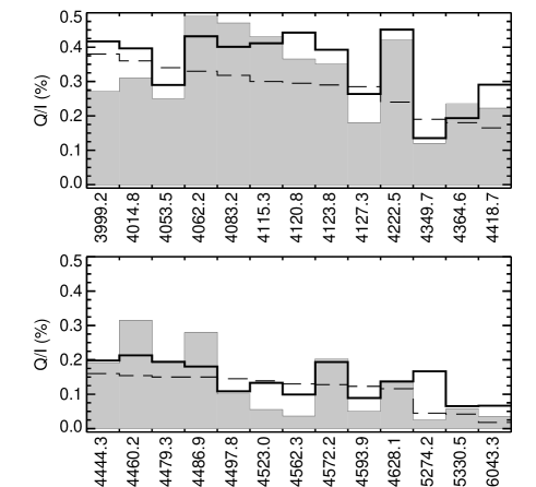
Figure 1: Main polarization features in the visible line spectrum of Ce ii. Shadowed bars and dashed line represent, respectively, the fractional polarization in the spectral lines and in the adjacent continuum observed near the solar limb ($\mu=0.1$), as reported by Gandorfer (2000, 2002). The heavy line represents the fractional polarization as calculated in this work ($\mu\rightarrow 0$). For representation purpouses the calculated fractional polarization has been scaled by an arbitrary factor $\alpha=0.08$ and added to the continuum fractional polarization (see Eq. (15) with $\eta_{I}^{\rm line}/\eta_{I}^{\rm cont}=\alpha$).

Expression (14) may be further developed taking into account that rare earths show very weak lines in the solar spectrum. Thus, in the limit $\eta_{I}^{\rm line}/\eta_{I}^{\rm cont}\ll 1$, Eq. (14) leads to

$$\frac{Q}{I}\,\approx\,\left(\frac{Q}{I}\right)^{\rm cont}+\left[\frac{\epsilon_{Q}^{\rm line}}{\epsilon_{I}^{\rm line}}\frac{S^{\rm line}}{B}-\frac{\eta_{Q}^{\rm line}}{\eta_{I}^{\rm line}}\right]\frac{\eta_{I}^{\rm line}}{\eta_{I}^{\rm cont}},$$ (15)

where $S^{\rm line}$ and $B$ are the line and continuum source functions, respectively. The expression between brackets in Eq. (15) is easy to evaluate once the $\rho^{0}_{0}$ and $\rho^{2}_{0}$ elements of the levels involved are known because $\epsilon_{i}^{\rm line}$ and $\eta_{i}^{\rm line}$ are given in Eqs. (9)-(12) above and, assuming that the continuum source function is the Planck function, we have

$$\frac{S^{\rm line}}{B}=\left(\frac{2J_{\ell}+1}{2J_{u}+1}\right)^{1/2}\frac{\rho^{0}_{0}(u)}{\rho^{0}_{0}(\ell)}({\rm e}^{h\nu/k_{\rm B}T}-1),$$ (16)

where we assume a temperature $T=5800$ K. The ratio ${\eta_{I}^{\rm line}}/{\eta_{I}^{\rm cont}}$ in Eq. (15) depends critically on the details of the line formation and cannot be calculated without a true radiative transfer treatment. Consistently with our simplified transfer model, we assume that this ratio is given by some arbitrary value $\alpha$, identical for all the lines, and we take the value that better match the observations. More generally, $\alpha$ also accounts for any systematic effect (identical for all the lines), not considered in our modeling like, for instance, the lower polarization degree for on-disk observations with respect to the tangential limit, and the broadening of line profiles.

Figure 1 shows the line core polarization in 26 lines of the Ce ii solar spectrum (shadow bars) as reported by Gandorfer (2000, 2002; to be referred to as the Atlas hereafter). The lines have been selected as those showing a clear polarization peak, either above the continuum or as a depolarization feature in the Atlas. We have avoided lines with severe blends that do not allow a clear assignment of the polarization signal. In particular, we have avoided lines having blends with species that are known to have notable scattering polarization signals (e.g., Ti i, Cr i, molecules), or lines that lie on a highly structured polarization background (e.g., on the wings of the H- and K-lines of Ca ii). We point out, however, that sometimes it is possible to ascribe clearly some $Q/I$ signal to a line despite an intensity blend. Those lines have also been included in the study.

The heavy line in Fig. 1 shows the polarization signal in each transition calculated according to the analysis above (Eqs. (3)-(15)). Our simplified scattering polarization modeling is able to reproduce the sign of most of the selected lines and roughly the relative $Q/I$ signals among lines. A quantitative evaluation of the agreement between the observed polarization pattern and the theoretical estimate may be given through the correlation factor $r=\sum p_{i}q_{i}/(\sum p_{i}^{2}\sum q_{i}^{2})^{1/2}$, where $p_{i}$ and $q_{i}$ correspond to the observed and theoretical fractional polarization in the $i$-th line, referred to the continuum. For the case shown in Fig. 1, $r=0.72$.

A better modeling of the observed pattern requires to include depolarizing collisions and turbulent magnetic fields. A detailed treatment of depolarizing collisions is not possible because of the lack of data. Some progress is indeed going on on the theoretical side (e.g., Derouich et al. 2003, 2004; Kerkeni 2002), but no reliable calculations exist (to the authors’ knowledge) of depolarizing rates in rare earth atoms. Nonetheless, much qualitative understanding on their role may be gained by proceeding as in Papers i; we just consider one and the same depolarizing collisional rate $D$ for all the statistical tensors with $K\neq 0$ in all the levels and we add a rate of the form $-D\rho^{K}_{0}(i)$ to the statistical equilibrium equation of each $\rho^{K}_{0}(i)$ element with $K\neq 0$.

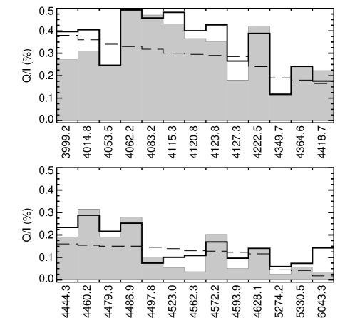
Figure 2: Same as Fig. 1 with a common depolarizing rate $D=10^{6}$ s^-1 for all the levels of the Ce ii model, and $\alpha=0.12$.

Figure 2 shows the fractional polarization calculated assuming a depolarizing rate $D=10^{6}$ s^-1 for all the atomic levels (heavy line). The agreement with the observed polarization pattern (shadow bars) is better than in the $D=0$ case (cf. Fig. 1); quantitatively, this is reflected in a larger correlation factor $r=0.83$. However, the agreement does not improve further for increasingly larger depolarizing rates but, on the contrary, it degrades, which puts an upper limit to the depolarizing collisional rate at about $\sim 10^{6}$ s^-1.

A depolarizing rate $D=10^{6}$ s^-1 leaves the atomic polarization of the lowermost levels (ground and metastable) of Ce ii at about one fifth of the atomic polarization in the absence of depolarizing processes. This is interesting because a microturbulent magnetic field may also depolarize an atomic level whenever its corresponding Larmor frequency $\nu_{L}$ is of the order of the relaxation rates of the level (i.e., the inverse of its mean life-time $\tau$) or larger. But, differently from the case of collisions, the depolarization saturates when $\nu_{L}\gg 1/\tau$, and the atomic polarization of the level remains at a constant value that is one fifth that of the non magnetic case (see Appendix). Therefore, the results in Fig. 2 are consistent with the presence of a turbulent magnetic field in the saturation regime of the Hanle effect for the lower levels. The lowermost levels of our Ce ii model atom have mean life times $\tau\approx$1-8$\times 10^{-6}$ s; the turbulent magnetic field required for reaching the saturation regime of the lowermost levels of Ce ii is hence of the order of 0.1-0.8 gauss.

On the other hand, the magnetic field cannot be so strong to saturate also the upper levels of the transitions, or the fractional polarization pattern would be exactly as in the non magnetic case but reduced to one fifth, and therefore, $r$ would degrade again to 0.72. The upper levels of the transitions considered in this study have mean lifetimes $\tau\approx 4$-6$\times 10^{-9}$ s; most of these levels saturate with fields $B\gtrsim$ 200 gauss, all of them when $B\gtrsim$ 300 gauss.

3 Conclusions

Rare earths are atoms with a complex level structure whose scattering polarization patterns cannot be understood using simple two level approximations. Moreover, in astrophysical environments (and in the solar atmosphere in particular), many transitions are excited simultaneously and the population and atomic polarization of a level depend on the balance between all the absorption and emission processes involving the level.

Here, we have considered the generation and distribution of atomic alignment in a multilevel atomic model of Ce ii when it is illuminated by a solar phostospheric-like radiation field. We have seen that the ensuing polarization of the scattered light is in good agreement with the observed polarization pattern of Ce ii. In particular, our model is capable of explaining the strongest polarized signals, as well as the sign of the polarization signal observed in most of the lines selected in this study.

With a simple analysis of the role of depolarizing collisions we have shown that the best agreement with observations is achieved at depolarizing rates $D=10^{6}$ s^-1, thus establishing an upper limit to these collisions. In this regime, the lowermost levels of ionized cerium show an atomic polarization that is of the order of one fifth of that which would be present in the absence of any depolarizing mechanisms. We interpret this fact as an indication of the presence of volume-filling microturbulent magnetic field of strength $B\gtrsim 0.8$ gauss (the saturation regime of the Hanle effect for the lowermost levels). Since in the presence of a magnetic field strong enough to saturate also the upper levels the relative polarization of the lines would match observations exactly as in the non magnetic case (which is not the best fit), we conclude that the magnetic field is not saturating the upper levels and hence the magnetic field must be $B\lesssim$ 200–300 gauss.

In summary, we have given a theoretical interpretation of the second solar spectrum of Ce ii and shown that it is a promising diagnostic tool to probe the magnetism and thermodynamics of the solar atmosphere. However, we cannot proceed much further with the elementary methods used in this paper.

Two are the main limitations of this research that must be addressed next. First, the full radiative transfer problem must be solved, thus allowing for different heights of formation of the lines. Second, the role of the magnetic field must be included consistently beyond the analogy with depolarizing collisions used here. The results of these investigations will be presented in forthcoming papers.

Appendix A Saturation Regime of the Hanle Effect from a Microturbulent Field

When a magnetic field is present in an otherwise axisymmetric enviroment, it is not possible, in general, to characterize the excitation state of the atoms only with the populations of the individual magnetic sublevels (or equivalently, through the statistical tensors $\rho^{K}_{0}$). Taking the quantization axis along the direction of the magnetic field, the radiation field is characterized through the $J^{K}_{Q}$ components ($K=0,2$, $Q=-K,...,K$), where the $Q\neq 0$ elements are azimuthal averages of the intensity of the radiation field (e.g., Landi Degl’Innocenti & Landolfi 2004). Correspondingly, the atomic excitation is described by the larger set of statistical tensors $\rho^{K}_{Q}$, ($K=0,2,4,...,K_{\rm max}$, $Q=-K,...,K$; $K_{\rm max}=2J$ or $2J-1$ for integer or half-integer $J$, respectively), where the $Q\neq 0$ elements correspond to quantum coherences between magnetic sublevels (e.g., Fano 1957; Landi Degl’Innocenti & Landolfi 2004). If the radiation field satisfies the condition $J^{K}_{Q}/J^{0}_{0}\ll 1$ (for, $K,Q\neq 0$), which is typically the case in stellar atmospheres, then $\rho^{K}_{Q}/\rho^{0}_{0}\ll 1$ (for, $K,Q\neq 0$), and a perturbative treatment of the statistical equilibrium equations can be performed (weak anisotropy approximation; see Landi Degl’Innocenti 1984; Landi Degl’Innocenti & Landolfi 2004, Sect. 10.13). Then, to first order, the statistical equilibrium equations in the magnetic field reference system do not couple the $\rho^{K}_{Q}$ components with $\rho^{K^{\prime}}_{Q^{\prime}}$ components having $Q\neq Q^{\prime}$.

Let ${\cal V}$ and ${\cal M}$ be the reference systems with the quantization axis directed along the vertical and the magnetic field, respectively; let R be the rotation taking ${\cal V}$ into ${\cal M}$, and ${\cal D}^{K}_{QQ^{\prime}}(R)$ ($Q,Q^{\prime}=-K,...,K$) the corresponding rotation matrix (e.g., Brink & Satchler 1968). Let $[\rho^{2}_{0}]^{\circ}$ be the alignment of a level in the reference system ${\cal V}$, for zero magnetic field. In the reference system ${\cal M}$, it turns out that $[\rho^{2}_{0}]^{\rm m}={\cal D}^{2}_{00}(R)[\rho^{2}_{0}]^{\circ}$. This is true even if the magnetic field is not zero, since it does not alter $[\rho^{2}_{0}]^{\rm m}$ directly, and $[\rho^{2}_{0}]^{\rm m}$ is decoupled from other $[\rho^{2}_{Q}]^{\rm m}$ components with $Q\neq 0$ (see above). Moreover, if the Larmor frequency $\nu_{L}$ is much larger than the radiative rates ${\cal R}_{i}$ of the level, this is the only non zero density matrix element because $[\rho^{K}_{Q}]^{\rm m}\rightarrow 0$ for components $Q\neq 0$. Finally, passing from ${\cal M}$ to ${\cal V}$, $[\rho^{K}_{Q}]={\cal D}^{K}_{Q0}(R)^{*}{\cal D}^{K}_{00}(R)[\rho^{2}_{0}]^{\circ}$. Averaging over all the directions of the turbulent field, $[\rho^{2}_{Q}]=\delta_{Q0}[\rho^{2}_{0}]^{\circ}/5$. Therefore, the alignment of a level in the saturated Hanle effect regime ($\nu_{L}\gg{\cal R}_{i}$), is 1/5 of its ’non magnetic’ value.

Now, suppose there is magnetic field regime such that the atomic levels can be classified in two types; type A: levels in the saturated regime and type B: levels in the regime $\nu_{L}\ll{\cal R}_{i}$. The alignment of levels in set A is 1/5 of the value obtained by solving Eqs. (3)-(6). The alignment of the levels in set B is obtained solving a restricted system of equations under this constraint. Moreover, it can also be shown that the alignment of the levels in set B is the weighted average (with weights 1/5 and 4/5, respectively), of the value obtained by solving Eqs.(3)-(6), and of the value obtained by solving the same equations under the constraint of complete depolarization of the levels of set A.

The rationale for this problem is the following. Because of the large life-time difference between metastable and excited levels, the lower- and upper-level Hanle effect regimes are usually well separated ($\tau_{\ell}/\tau_{u}\sim A_{u\ell}/B_{\ell u}J^{0}_{0}\sim 100$ for two levels conected by an allowed visible transition). Therefore, there is a regime of magnetic fields in which metastable levels are completely saturated while excited levels remain essentially unaffected by the magnetic field. In some astrophysical enviroments the microscopic fields created by the motion of nearby ions may be large enough to saturate the Hanle effect of metastable levels. From a physical point of view, the zero (macroscopic) field case then corresponds to the solution of the problem just stated.

References

- (1) Asplund, M., Grevesse, N., & Sauval, A. J. 2005, in ASP Conf. Ser. 336, Cosmic Abundances as Records of Stellar Evolution and Nucleosynthesis, eds. Thomas G. Barnes iii and Frank N. Bash(San Francisco: ASP), p. 25; arXiv:astro-ph/0410214v2
- (2) Brink, D. M., & Satchler, G. R. 1968, Angular Momentum (Oxford: Clarendon Press)
- (3) Cox, A.N. 2000, Allen’s Astrophysical Quantities 4th ed. (New York: Springer Verlag and AIP Press)
- (4) Derouich, M., Sahal-Bréchot, S., Barklem, P. S., & O’Mara, B. J. 2003, A&A, 404, 763
- (5) Derouich, M., Sahal-Bréchot, S., & Barklem, P. S. 2004, A&A, 426, 707
- (6) van Diest, H. 1980, A&A, 83, 378
- (7) Fano, U. 1957, Rev. Mod. Phys., 29, 74
- (8) Gandorfer, A. 2000, The Second Solar Spectrum: A high spectral resolution polarimetric survey of scattering polarization at the solar limb in graphical representation. Volume i: 4625 Å to 6995 Å (Zürich: vdf Hochschulverlag AG an der ETH)
- (9) Gandorfer, A. 2002, The Second Solar Spectrum: A high spectral resolution polarimetric survey of scattering polarization at the solar limb in graphical representation. Volume ii: 3910 Å to 4630 Å (Zürich: vdf Hochschulverlag AG an der ETH)
- (10) Irwin, A. W. 1981, ApJS, 45, 621
- (11) Kerkeni, B. 2002, A&A, 390, 783
- (12) Landi Degl’Innocenti, E. 1984, Sol. Phys., 91, 1
- (13) Landi Degl’Innocenti, E. & Landolfi, M. 2004, Polarization in Spectral Lines (Dordrecht: Kluwer)
- (14) Manso Sainz, R., & Landi Degl’Innocenti, E. 2002, A&A, 394, 1093 (Paper ia)
- (15) Manso Sainz, R., & Landi Degl’Innocenti, E. 2003, in ASP Conf. Ser. 307, Solar Polarization 3, eds. J. Trujillo Bueno and J. Sánchez Almeida (San Francisco: ASP), 425 (Paper ib)
- (16) Martin, W. C., Zalubas, R., & Hagan, L. 1978, Atomic Energy Levels—The Rare-Earth Elements, Natl. Stand. Ref. Data Ser., Natl. Bur. Stand. (U.S.) monograph 60.
- (17) Palmeri, P., Quinet, P., Wyart, J.-F., & Biémont, E. 2000, Phys. Scripta, 61, 323
- (18) Stenflo, J.O., & Keller, C.U. 1996, Nature, 382, 588
- (19) Stenflo, J.O., & Keller, C.U. 1997, A&A, 321, 927
- (20) Trujillo Bueno, J. 2003, in Solar Polarization 3, ed. J. Trujillo Bueno & J. Sánchez Almeida, ASP Conf. Ser. Vol. 307, 407
- (21) Vernazza, J. E., Avrett, E. H., & Loeser, R. 1976, ApJS, 30, 1
- (22) Zhang, Z. G., Svanberg, S., Zhankui Jiang, Palmeri, P., Quinet, P., & Biémont, E. 2001, Phys. Scripta, 63, 122