CHAOS AND THE DYNAMICAL EVOLUTION OF BARRED GALAXIES

Abstract

The dynamical evolution of barred galaxies depends crucially on the fraction and their spacial distribution of chaotic orbits in them. In order to distinguish between the two kinds of orbits, we use the Smaller Alignment Index (SALI) method, a very powerful method which can be applied to problems of galactic dynamics. Using model potentials, and taking into account the full 3D distribution of matter, we discuss how the distribution of chaotic orbits depends on the main model parameters, like the mass of the various components and the bar axial ratio.

^† Observatoire Astronomique de Marseille-Provence (OAMP), FRANCE.
^∗ Center for Research and Applications of Nonlinear Systems (CRANS),
Department of Mathematics, University of Patras, GREECE.

1 Introduction

The distinction between ordered and chaotic motion in dynamical systems is fundamental in many areas of applied sciences. This distinction is particularly difficult in systems with many degrees of freedom (dof), basically because it is not feasible to visualize their phase space. Thus, we need fast and accurate tools to give us information about the chaotic or ordered character of the orbits, especially for conservative systems. In this work we focus our attention on the method of the Smaller ALignment Index (SALI) [1], or, as elsewhere called Alignment Index (AI) [3] and we present some applications of the index in Ferrers barred galaxy potentials of 2 and 3 dof. In order to compute the SALI for a given orbit, one has to follow the time evolution of the orbit itself and also of two deviation vectors $v_{1}$ and $v_{2}$, which initially point in two different directions. At every time step the two deviation vectors are normalized and the SALI is then computed as:

$$SALI(t)=min\{\|\frac{v_{1}(t)}{\|v_{1}(t)\|}+\frac{v_{2}(t)}{\|v_{2}(t)\|}\|,\|\frac{v_{1}(t)}{\|v_{1}(t)\|}-\frac{v_{2}(t)}{\|v_{2}(t)\|}\|\}.$$ (1)

In 2 and 3 dof Hamiltonian systems the distinction between ordered and chaotic motion is easy because the ordered motion occurs on a 2D or 4D torus, respectively, to which any initial deviation vector becomes almost tangent after a short transient period. The behavior of SALI is also discussed in [2], where some applications were also presented.

Our goal is to study how the fraction of the ordered and chaotic trajectories, in 2 and 3 dof, depends on some major parameters of the models. We use a 2 dof and 3 dof barred potential, which rotates around its z-axis. The system is rotating with an angular speed $\Omega_{b}$ and can be described by the following Hamiltonian form:

$$H=\frac{1}{2}(p_{x}^{2}+p_{y}^{2}+p_{z}^{2})+V(x,y,z)-\Omega_{b}(xp_{y}-yp_{x}).$$ (2)

Our model potential consists of a Miyamoto disc, a Plummer sphere and a Ferrers bar.

2 Applications in the 2D case

We first apply the SALI index to the 2 dof barred potential. In this case, we can have a Poincaré Surface of Section (PSS) and can check the effectiveness of the SALI, by comparing the results.

In figure 1, we present two orbits of different kind: (i) $(x,y,p_{x},p_{y})=(1.5,0,p_{x}(H),0)$ and (ii) $(x,y,p_{x},p_{y})=(-0.9,0,p_{x}(H),0)$. For this application $H=-0.3$. In panels a) and b) of figure 1, we show the orbit projections in the $(x,y)$-plane and in panel c) we draw their corresponding PSS, where we can see that the chaotic orbit (i) tends to fill with scattered points the available part of the plane $(x,\dot{x})$ and that the ordered orbit (ii) creates a closed invariant curve. Finally, in panel d) we apply the SALI method for these two orbits. For the chaotic one, the SALI tends to zero $(10^{-16})$ exponentially after some time steps while for the regular orbit, it fluctuates around a positive number. By choosing initial conditions on the line $\dot{x}=0$ of the PSS and calculating the values of the SALI, we can detect very small regions of stability that can not be visualized easily by the PSS method. Repeating this for many values of the energy, we are able to follow the change of the fraction of chaotic and ordered orbits in the phase space as the energy of the system varies.

3 Applications in the 3D case

A similar study can be made for the 3 dof case of the barred potential. We first try a basic model and we vary two parameters, the length of the short z-axis $c$ and the mass $M_{bar}$ of the bar. The initial conditions are given in two ways: a) in the plane $(x,p_{y},z)$ with $(y,p_{x},p_{z})=(0,0,0)$ and b) in the plane $(x,p_{y},p_{z})$ with $(y,z,p_{z})=(0,0,0)$. In both cases, we find similar results. As the mass $M_{bar}$ of the bar increases, the percentage of the chaotic orbits increases as well. This is in good agreement with the results found for 2 dof by Athanassoula et al. (1983). In the other case, we find that when the length of the short z-axis $c$ of the bar increases (keeping the $M_{bar}$ constant), the system presents more regular behaviour than in the initial model.

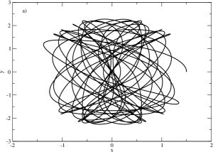
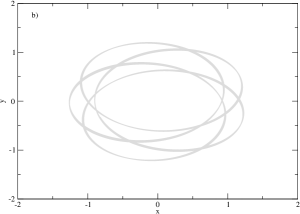
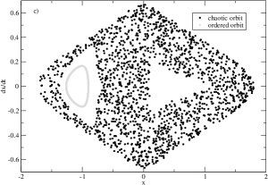
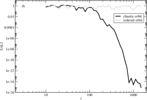
Figure 1: Projections of the orbits (i) and (ii) in the $(x,y)$-plane (panels a), b)). PSS of these two orbits in panel c). Behaviour of the SALI of the same orbits (panel d)).

4 Conclusions

In this paper, we applied the SALI method in the Ferrers barred galaxy models of 2 and 3 dof. We presented and discussed our results comparing the index with traditional methods, such as the PSS method for the 2 dof and showed its effectiveness. We also, calculated percentages of chaotic and regular orbits and how they change with the main model parameters, for the 3 dof case.

Acknowledgements.  Thanos Manos was partially supported by Karatheodory graduate student fellowship No B395 of the University of Patras and by Marie - Curie fellowship No HPMT-CT-2001-00338.

References

- [1] Skokos Ch., 2001, J. Phys. A: Math. Gen., 34, 10029
- [2] Skokos Ch., Antonopoulos C., Bountis T. and Vrahatis, M., 2004, J. Phys. A, 37, 6269
- [3] Voglis N., Kalapotharakos C. and Stavropoulos I., 2002, Mon. Not. R. Astron. Soc. 337, 619
- [4] Athanassoula E., Bienayme O., Martinet L. and Pfenniger D., 1983, Astr. Astroph. 127, 349