Non-Gaussian Foreground Residuals of the WMAP First Year Maps

Abstract

We investigate the effect of foreground residuals in the WMAP data (Bennett et al., 2003a) by adding foreground contamination to Gaussian ensembles of CMB signal and noise maps. We evaluate a set of non-Gaussian estimators on the contaminated ensembles to determine with what accuracy any residual in the data can be constrained using higher order statistics. We apply the estimators to the raw and cleaned Q, V, and W band first year maps. The foreground subtraction method applied to clean the data in Bennett et al. (2003b) appears to have induced a correlation between the power spectra and normalized bispectra of the maps which is absent in Gaussian simulations. It also appears to increase the correlation between the $\Delta\ell=1$ inter-$\ell$ bispectrum of the cleaned maps and the foreground templates. In a number of cases the significance of the effect is above the 98% confidence level.

1 Introduction

Over the past few years there has been a heightened interest in testing the statistical properties of Cosmic Microwave Background (CMB) data. The process has been accelerated by the release of the WMAP first year results. The WMAP data provide the first ever, full-sky maps which are signal dominated up to scales of a few degrees. Thus, for the first time we can test the Gaussianity and isotropy assumptions of the cosmological signal over large scales in the sample variance limit.

Ever since the release of the COBE-DMR results (Bennett et al., 1996) a consensus has been hard to reach on tests of non-Gaussianity with some studies reporting null results (Kogut et al., 1996; Contaldi et al., 2000; Sandvik & Magueijo, 2001) while others claimed detections of non-Gaussian features (Ferreira et al., 1998; Magueijo, 2000; Novikov, Feldman & Shandarin, 1998; Pando et al., 1998). With the release of the WMAP first year results a limit on the non-Gaussianity of primordial perturbations in the form of an estimate of the non-linear factor $f_{\rm NL}$ was obtained by Komatsu et al. (2003). However a number of authors (Bielewicz et al., 2004; Eriksen et al., 2004a; Coles et al., 2004; Park, 2004; Copi et al., 2004; de Oliveira-Costa et al., 2004; Land & Magueijo, 2005; Efstathiou, 2003; Roukema et al., 2004; Eriksen et al., 2005; Jaffe et al., 2005) have also reported analysis of the maps that suggest violations of the Gaussian or isotropic nature of the signal.

One of problems with testing Gaussianity is that one can devise a plethora of tests to probe the infinite degrees of non-Gaussianity, therefore different tests represent different perspectives on the statistical patterns of the signal. For WMAP there are already a number of detections of so called anomalies, most pointing to different unexpected features in the microwave sky. The most documented case (Peiris et al., 2003; Efstathiou, 2003; Slosar & Seljak, 2004; de Oliveira-Costa et al., 2004; Eriksen et al., 2004a) is the low amplitude of the quadrupole and octupole in comparison to the inflationary prediction, something we can categorize as amplitude anomalies. Although it is simple to design inflationary spectra with sharp features which reproduce, more or less closely, the amplitude anomaly (see e.g. Contaldi et al. (2003); Bridle et al. (2003); Salopek et al. (1989)) these invariably suffer fine tuning problems. Another approach is to relate the anomaly to the breakdown of statistical isotropy or Gaussianity.

Other reported features relate to the correlation of phases in the multipole coefficients which are an indication of non-Gaussianity. These can be dubbed phase anomalies. One example is the hemisphere asymmetries (Eriksen et al., 2004a); the northern ecliptic hemisphere is practically flat while the southern hemisphere displays relatively high fluctuations in the power spectrum. Other functions, such as the bispectrum (Land & Magueijo, 2005) and n-point correlation functions (Eriksen et al., 2005) also show related asymmetries. Furthermore, there is the anomalous morphology of several multipoles, in particular, the striking planarity of the quadrupole and octupole and the strong alignment between their preferred directions (de Oliveira-Costa et al., 2004). Overall, there is a strong motivation to continue probing the statistical properties of the data and find possible sources for these signals, be it instrumental, astrophysical or cosmological.

The first test to have provided indications of possible non-Gaussian features in the CMB data was reported by Ferreira et al. (1998) and Magueijo (2000) using a bispectrum estimator, the fourier analog of the three point function. Both those detections were later found to be caused by systematic effects rather than by cosmological source as reported by Banday et al. (2000). For the case of the bispectrum signal detected by Magueijo (2000), which used an estimator tuned to detect correlations between neighbouring angular scales, finding the source of the signal had to wait for the release of the high precision WMAP data (Bennett et al., 2003a) which was able to provide a comparative test of the cosmological signal. The WMAP data did not reproduce COBE’s result and systematic errors were found to be the cause (Magueijo & Medeiros, 2004). The WMAP data was later analysed with the bispectrum in more detail by Land & Magueijo (2005). In that paper, the bispectrum of the clean, coadded maps was analysed and a connection between the hemisphere asymmetries in the 3-point correlation function and the bispectrum was established, although the full sky as a whole was found to be consistent with Gaussianity.

In this paper, we study the effect that foreground contaminations have on bispectrum estimators. In section 2 we define a set of bispectrum estimators with set $\ell$ configurations. In section 3 we describe the template dust, free-free and synchrotron maps used to characterize the effect on the bispectrum. In section 4 we determine the distribution of the estimators in the presence of residual foregrounds with different amplitudes and discuss the application of this method to detect residuals in the data by introducing a number of statistical and correlation measures. In section 5 we discuss the application of the the statistical tools developed in the previous sections to the raw and cleaned WMAP first year maps. We conclude with a discussion of our method and results in section 6.

2 The Angular Bispectrum

We now introduce the angular bispectrum estimator (Ferreira et al., 1998). The bispectrum is related to the third order moment of the spherical harmonic coefficients $a_{\ell m}$ of a temperature fluctuation map $\Delta T({\bf\hat{n}})/T$. The coefficients describe the usual expansion of the map over the set of spherical harmonics $Y_{\ell m}({\bf\hat{n}})$ as

$$\frac{\Delta T}{T}({\bf\hat{n}})=\sum_{\ell m}a_{\ell m}Y_{\ell m}({\bf\hat{n}}).$$ (1)

Given a map, either in pixel space or harmonic space, and assuming statistical isotropy, one can construct a set hierarchy of rotationally invariant statistical quantities characterizing the pattern of fluctuations in the maps. These are the n-point correlation functions in the temperature fluctuations $\langle\frac{\Delta T}{T}({\bf\hat{m}})\frac{\Delta T}{T}({\bf\hat{n}})...\frac{\Delta T}{T}({\bf\hat{p}})\rangle$ or in the spherical harmonic coefficients, $\langle a_{\ell_{1}m_{1}}a_{\ell_{2}m_{2}}...a_{\ell_{n}m_{n}}\rangle$.

The unique quadratic invariant is the angular power spectrum defined as $\langle a_{\ell_{1}m_{1}}a^{\star}_{\ell_{2}m_{2}}\rangle=\delta_{\ell_{1}\ell_{2}}\delta_{m_{1}m_{2}}C_{\ell}$, whose estimator can be written as ${\hat{C}}_{\ell}=\frac{1}{2\ell+1}\sum_{m}|a_{\ell m}|^{2}$. This gives a measure of the overall intensity for each multipole $\ell$. Following Ferreira et al. (1998), the most general cubic invariant defines the angle averaged bispectrum,

$$\left<a_{\ell_{1}m_{1}}a_{\ell_{2}m_{2}}a_{\ell_{3}m_{3}}\right>=B_{\ell_{1}\ell_{2}\ell_{3}}\left(\begin{array}[]{ccc}\ell_{1}&\ell_{2}&\ell_{3}\\ m_{1}&m_{2}&m_{3}\end{array}\right),$$ (2)

where the $(\ldots)$ is the Wigner $3J$ symbol. Parity invariance of the spherical harmonic functions dictates that the bispectrum be non-zero only for multipole combinations where the sum $\ell_{1}+\ell_{2}+\ell_{3}$ is even. An unbiased estimator (for the full sky) can be evaluated as

$${\hat{B}}_{\ell_{1}\ell_{2}\ell_{3}} = \frac{{\cal N}^{-1}_{\ell_{1}\ell_{2}\ell_{3}}}{\sqrt{4\pi}}\sum_{m_{1}m_{2}m_{3}}\left(\begin{array}[]{ccc}\ell_{1}&\ell_{2}&\ell_{3}\\ m_{1}&m_{2}&m_{3}\end{array}\right)\times$$

$$a_{\ell_{1}m_{1}}a_{\ell_{2}m_{2}}a_{\ell_{3}m_{3}},$$

with the normalization factor defined as

$${\cal N}_{\ell_{1}\ell_{2}\ell_{3}} = {\left(\begin{array}[]{ccc}\ell_{1}&\ell_{2}&\ell_{3}\\ 0&0&0\end{array}\right)}\times$$

$$\sqrt{\frac{(2\ell_{1}+1)(2\ell_{2}+1)(2\ell_{3}+1)}{4\pi}}.$$

The bispectrum can be related to the three-point correlation functions of the map just as the power spectrum $C_{\ell}$ can be related to the correlation function $C(\theta)$ through the well known expression

$$C(\theta)=\frac{1}{4\pi}\sum_{\ell}(2\ell+1)C_{\ell}P_{\ell}(\cos\theta).$$ (9)

For example, the pseudo-collapsed, three-point correlation function, $C^{(3)}(\theta)=\langle\frac{\Delta T}{T}({\bf\hat{n}})^{2}\frac{\Delta T}{T}({\bf\hat{m}})\rangle$, is related to our definition of the bispectrum $B_{\ell_{1}\ell_{2}\ell_{3}}$ as

$$C^{(3)}(\theta)=\frac{1}{4\pi}\sum_{\ell_{1}\ell_{2}\ell_{3}}{\cal N}_{\ell_{1}\ell_{2}\ell_{3}}B_{\ell_{1}\ell_{2}\ell_{3}}P_{\ell_{3}}(\cos\theta),$$ (10)

where ${\bf\hat{n}}\cdot{\bf\hat{m}}=\cos\theta$.

It is important to use both tools, the bispectrum and the three-point correlation function, to probe the sky maps as they have the capacity to highlight different features of the data. In principle, harmonic space based methods are preferred for the study of primordial fluctuations whereas real space methods are more sensitive to systematics and foregrounds, which are strongly localized in real space. In addition, the three-point correlation function is intrinsically very sensitive to the low-$\ell$ modes, whereas the bispectrum can pick up different degrees of freedom with respect to the different mode correlations we want to probe

For the choice $\ell_{1}=\ell_{2}=\ell_{3}=\ell$ we can define the single-$\ell$ bispectrum ${\hat{B}_{\ell}}=\hat{B}_{\ell\,\ell\,\ell}$ (Ferreira et al., 1998), which probes correlations between different $m$’s. Other bispectrum components are sensitive to correlations between different scales $\ell$. This can be extended to study correlations from different angular scales. The simplest of these is the $\Delta\ell=1$ inter-$\ell$ bispectrum between neighbouring multipoles defined as $\hat{B}_{\ell-1\,\ell\,\ell+1}$ (Magueijo, 2000). It is convenient to consider estimators normalized by their expected Gaussian variance $\hat{C}_{\ell_{1}}\hat{C}_{\ell_{2}}\hat{C}_{\ell_{3}}$ which have been shown to be more optimal and more Gaussian distributed than the unnormalized estimators, and are not sensitive to the overall power in the maps. Here we will introduce the $\hat{I}_{\ell}$,$\hat{J}_{\ell}$, and $\hat{K}_{\ell}$ bispectra defined as

$$I^{3}_{\ell}={{\hat{B}}_{\ell}\over({\hat{C}}_{\ell})^{3/2}},\ \ J^{3}_{\ell}={\hat{B}_{\ell-1\,\ell\,\ell+1}\over({\hat{C}}_{\ell-1}{\hat{C}}_{\ell}{\hat{C}}_{\ell+1})^{1/2}},$$ (11)

and

$$K^{3}_{\ell}={\hat{B}_{\ell-2\,\ell\,\ell+2}\over({\hat{C}}_{\ell-2}{\hat{C}}_{\ell}{\hat{C}}_{\ell+2})^{1/2}},$$ (12)

where have extended the formalism to a separation $\Delta\ell=2$ to probe signals with both odd and even parity in the inter-$\ell$ correlations.

3 Foreground Templates

The standard method of foreground removal used by cosmologists makes use of a set of template maps for each of the dominant sources of foreground contamination in the CMB frequency maps. These are maps obtained from independent astronomical full-sky observations at frequencies where the respective mechanisms of emission are supposed to be dominant. These templates are the H $\alpha$ map (Finkbeiner, 2003), for the free-free emission, the 408 MHz Haslam map (Haslam et al., 1981), for the synchrotron emission, and the FDS 94 GHz dust map (Schlegel et al., 1998). These are then subtracted from the WMAP data with coupling coefficients determined by cross correlating with the observed maps in the Q (41 GHz), V (61 GHz), and W (94 GHz) bands. Nevertheless the templates are a poor approximation of the of the real sky near the galactic plane, so a Kp2 mask must still be used in the analysis. The method is described in Bennett et al. (2003b) and Komatsu et al. (2002);

$$\overline{T}_{Q} = T_{Q}-1.044\,[1.036\,T^{\rm FDS}+\frac{1.923}{\eta}\,T^{H\alpha}$$

$$+1.006\,T^{\rm Sync}],$$

$$\overline{T}_{V} = T_{V}-1.100\,[0.619\,T^{\rm FDS}+\frac{1.923}{\eta}\,\left(\frac{\nu_{V}}{\nu_{Q}}\right)^{-2.15}\,T^{H\alpha}$$ (13)

$$+1.006\,\left(\frac{\nu_{V}}{\nu_{Q}}\right)^{-2.7}\,T^{\rm Sync}],$$

$$\overline{T}_{W} = T_{W}-1.251[0.873\,T^{\rm FDS}+\frac{1.923}{\eta}\,\left(\frac{\nu_{W}}{\nu_{Q}}\right)^{-2.15}\,T^{H\alpha}$$

$$+1.006\,\left(\frac{\nu_{W}}{\nu_{Q}}\right)^{-2.7}\,T^{\rm Sync}],$$

where $\eta$ is a correction factor due to reddening in the free-free template and $\nu_{Q}=40.7$ GHz, $\nu_{Q}=60.8$ GHz and $\nu_{W}=93.5$ GHz . The values in front of the left bracket convert the detector’s temperature to thermodynamic temperature. It is considered that this is a sufficiently good method to remove the foregrounds outside the Kp2 plane since it matches the correct amplitudes quite well, however the usual doubts remain, especially in the light of the alignment/low multipoles controversies. Another point one can make is that whereas this may be a satisfactory technique to correct the foregrounds at the power spectrum level, its effect on higher order statistics is unknown and may actually induce unexpected correlations.

4 The effect of foregrounds on the bispectrum

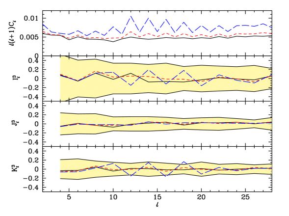
Figure 1: The average functions for the angular spectra of the simulations. Black (solid) is Gaussian, red (short-dashed) is for the contaminated simulations with $\alpha=0.5$ and blue (long-dashed) is for the contaminated simulations with $\alpha=1.0$. The top panel shows the power spectrum $\hat{C}_{\ell}$, second panel shows the single-$\ell$ bispectrum $I^{3}_{\ell}$, the third panel the $\Delta\ell=1$ inter-$\ell$ bispectrum $J^{3}_{\ell}$ and the bottom panel shows the $\Delta\ell=2$ inter-$\ell$ bispectrum $K^{3}_{\ell}$. The shaded regions represent the Gaussian variance measured directly from the ensemble of simulations. For the Gaussian simulations, the average power spectrum is just the input $\Lambda$CDM power spectrum and the average bispectra is effectively zero. On the other hand, the average angular spectra of the contaminated simulations have an emerging pattern of intermittency in both second- and third-order statistics. This intermittent pattern comes about due to the even parity of galactic foregrounds, ie, even modes are enhanced relatively to the odd modes. This can be seen in the significant increase of power in the even modes of the power spectrum. In terms of the bispectrum, we see that the $\Delta\ell=0$ and the $\Delta\ell=2$ inter-$\ell$ components will be more significantly enhanced than the $\Delta\ell=1$ inter-$\ell$ bispectrum because the latter includes correlations between even and odd modes.

We have generated a set of 3000 Gaussian, CMB simulations of the WMAP first year Q, V, and W maps in HEALPix(Górski et al., 2005) format with a resolution parameter $N_{\rm side}=512$. Each simulation is smoothed with the Q, V and W frequency channel beams and channel specific noise is added. We adopted the WMAP best-fit $\Lambda$CDM with running index power spectrum to generate the $a_{\ell m}$ coefficients of the maps. The Kp2 galactic mask is imposed on each map. The masked maps are then decomposed into spherical harmonic coefficients $a_{\ell m}$ using the Anafast routine. We then calculate the four spectra; namely the the power spectrum $\hat{C}_{\ell}$, single-$\ell$ bispectrum $I^{3}_{\ell}$, $\Delta\ell=1$ inter-$\ell$ bispectrum $J^{3}_{\ell}$ and $\Delta\ell=2$ inter-$\ell$ bispectrum $K^{3}_{\ell}$ as described in section 2.

We then add channel-specific foregrounds outside the Kp2 zone to the same set of Gaussian simulations with amplitudes set as in Eqn. (3). The addition of the foreground is scaled linearly by a factor $\alpha$ as

$$T_{\rm\{Q,V,W\}}=T_{\rm CMB}+\alpha\overline{T}_{\rm\{Q,V,W\}},$$ (14)

which we use to check the sensitivity of the bispectra to the foregrounds (typically $\alpha=1.0$ or $\alpha=0.5$). The power spectrum and bispectra are then calculated for the set of contaminated maps.

In Fig. 1 we show the mean angular spectra of the simulations obtained by averaging over the ensembles. We show the mean spectra for the Gaussian (solid, black) and the contaminated simulations for $\alpha=0.5$ (short-dashed, red) and $\alpha=1.0$ (long-dashed, blue). The shaded area shows the variance of the three bispectra obtained directly from the Gaussian simulations.

We see that even for the fully contaminated set of maps ($\alpha=1.0$) the average signal is not significantly larger than the expected Gaussian variance indicating that a detection would require averaging over a large number of modes. However we see some important distinguishing features in the signal in that it is sensitive to the parity of the multipole, being suppressed for odd $\ell$. This is due to the approximate symmetry of the foreground emission about the galactic plane which means that most of the signal will be in even $\ell$ modes since these have the same symmetry. This effect can be seen in all the spectra but most significant is the suppression of the odd inter-$\ell$ bispectrum $J^{3}_{\ell}$ with respect to the even inter-$\ell$ bispectra $I^{3}_{\ell}$ and $K^{3}_{\ell}$.

Another obvious feature of the even parity nature of the signal is the correlation between the spectra. In particular the absolute values of the $I^{3}_{\ell}$ and the $K^{3}_{\ell}$ are correlated with the structure visible in the fully contaminated power spectrum.

Overall the $K^{3}_{\ell}$ is the most sensitive statistic with the largest amplitude with respect to the Gaussian variance although still quite small even at $50\%$ contamination. We now describe a number of statistical estimators we use to test the detectability of the template matched foregrounds in the Q, V, and W channel maps.

4.1 Chi-Squared Test

Having seen how foregrounds affect the angular statistics of CMB maps, we can now devise specific tests to probe these properties on the bispectrum and test their sensitivity. The standard way to use the bispectrum as a test of general non-Gaussianity is to use a reduced $\chi^{2}$ statistic (Magueijo, 2000; Magueijo & Medeiros, 2004; Land & Magueijo, 2005). This is defined as

$$\chi^{2}={1\over N_{\ell}}{\sum_{\ell=\ell_{\rm min}}^{\ell_{\rm max}}\chi_{\ell}^{2}}={1\over N_{\ell}}\sum_{\ell=\ell_{\rm min}}^{\ell_{\rm max}}{{(X_{\ell}-\langle X_{\ell}\rangle)^{2}}\over{\sigma_{\ell}^{2}}}.$$ (15)

where $X_{\ell}$ is a given bispectrum statistic, $\langle X_{\ell}\rangle$ is its mean value computed over the Monte Carlo ensembles, and $\sigma_{\ell}^{2}$ is the variance for each angular scale. The $\chi^{2}$ test is a measure of the deviation of the observed data from the expected mean, weighted by the Gaussian variance of the estimator.

Foregrounds increase the amplitude of the bispectra foregrounds, but as shown in Fig. 1, we can see that only $K^{3}_{\ell}$ seems to stand of chance of significant detections since the average amplitude of the signal is comparable to the variance, unlike the other components of the bispectrum.

The detectability of the template matched signals using any of the bispectra can be tested by comparing the distribution of the $\chi^{2}$ values obtained from the contaminated simulations with that obtained from Gaussian simulations. We compute the $\chi^{2}$ values for the contaminated maps using the mean and the variance obtained from the Gaussian simulations, ie, the expected Gaussian functions.

We compare the distribution of the $\chi^{2}$ values for the Gaussian simulations against the distribution obtained for the simulations with contamination ($\alpha=1.0$). We concentrate on the Q band since it is the most contaminated frequency. The histograms of the $\chi^{2}$ are shown in the left column of Fig. 2. For the $I^{3}_{\ell}$ and $J^{3}_{\ell}$ spectra the histograms overlap completely. This means that the probability of finding contaminated simulations with a high $\chi^{2}$ is the same as for the Gaussian simulations indicating that the $\chi^{2}$ test is insensitive to the presence of foreground contaminations at this level. However the $K^{3}_{\ell}$ spectrum tells a different story. There is a significant shift between the two distributions which implies that this component of the bispectrum has more sensitivity to foregrounds.

The sensitivity can be quantified in terms of the fraction of the contaminated simulations (with $\alpha=1.$) with a $\chi^{2}$ larger value than 95.45 $\%$ (i.e. 2 $\sigma$) of the Gaussian simulations (with $\alpha=0$). The sensitivity for the $I^{3}_{\ell}$ and $J^{3}_{\ell}$ is low (¡ 0.05), whereas for $K^{3}_{\ell}$ the fraction increases to 0.355.

4.2 Template Correlation Test

A template matched statistic can be defined by correlating the observed bispectra in the data with those of the foreground templates. This is more sensitive to the structure in the template signal as opposed to the $\chi^{2}$ test introduced above. We define a cross correlation statistic $\rho$ as

$$\rho=\frac{\sum_{\ell=\ell_{\rm min}}^{\ell_{\rm max}}{X_{\ell}X^{F}_{\ell}}}{\left(\sum_{\ell=\ell_{\rm min}}^{\ell_{\rm max}}X_{\ell}^{2}\sum_{\ell=\ell_{\rm min}}^{\ell_{\rm max}}X^{F\,2}_{\ell}\right)^{1/2}}$$ (16)

where $X_{\ell}$ are the bispectra obtained from the data and the $X_{\ell}^{F}$ are those obtained from the foreground templates.

In the middle column of Fig. 2 we display the histograms for the $\rho$ values for the Gaussian simulations against the distribution obtained for the contaminated ($\alpha=1$) simulations of the Q band maps. The sensitivity has improved over the $\chi^{2}$ test, with the histograms of the input and output data sets being clearly shifted, meaning that there is a higher probability of detection of foregrounds using this method. Again the effect is stronger in the $K^{3}_{\ell}$. This result simply quantifies the statement that a matched template search for a contamination signal is more sensitive than a ‘blind’ statistic such as the $\chi^{2}$ test. The values for the sensitivity of the test are given in table 1 for all three WMAP bands.

4.3 Power Spectrum and Bispectra Cross-Correlation Test

For a Gaussian field, the normalized bispectrum is statistically uncorrelated with the power spectrum (Magueijo, 1995). However, foreground residuals in the map induce non-Gaussian correlations which in turn will induce correlations between the normalized bispectra and the power spectrum of the maps. This can provide another specific signature that one can use to detect the presence of foreground contamination.

For Gaussian simulations, the average power spectrum is just the input $\Lambda$CDM power spectrum and the bispectrum is effectively zero. On the other hand, the average angular spectra of the contaminated simulations have an emerging pattern of intermittency in both first- and second-order statistics. Correlations between the power spectrum and the bispectra therefore come about due to the even parity induced by the characteristic galactic foregrounds. This means that the even modes of the power spectrum will be correlated with the even modes of the bispectra, whereas odd modes will remain uncorrelated. In order to test this effect on the maps, we introduce the ${\rm R}$ correlation statistic defined as

$${\rm R}^{X}=\sum^{\ell_{\rm max}}_{\ell=\ell_{\rm min}}(-1)^{{\rm int}[\frac{\ell}{2}]+1}\hat{C}_{\ell}X_{\ell}$$ (17)

where $\hat{C}_{\ell}$ is the observed power spectrum. We have chosen $\ell_{\rm max}=30$ and $\ell_{\rm min}=4$ as we are interested in the large angular scales where the effects of foreground contamination will dominate. We use the absolute value of the bispectrum in order to avoid the discrimination between negative and positive correlations which would affect our sum. We are only interested in the discrimination between the existence of absolute correlations against null correlations between the $\hat{C}_{\ell}$ and the bispectra $X_{\ell}$.

Again we test the sensitivity of this method by computing a distribution of ${\rm R}$ for Gaussian ensembles against the contaminated ensembles. We make sure that for Gaussian ensembles we use the correlation of $\hat{C}^{\rm S+F}_{\ell}$ with $X^{\rm S}_{\ell}$ and for the contaminated ensemble the correlation of $\hat{C}^{\rm S+F}_{\ell}$ with $X^{\rm S+F}_{\ell}$ where $\rm S$ stands for the Gaussian CMB signal and $\rm S+F$ indicates contaminated ensembles. This allows us to cancel the effect of the increase of power due to foregrounds in the correlation of the two statistics between the two tests. The results for the contaminated ensemble, $\alpha=1$, are plotted in the right column of Fig. 2 and are summarized in table 1 for all three bands.

Table 1: Sensitivity of the $\rho$ and ${\rm R}$ tests in terms of the fraction of the contaminated simulations ($\alpha=1.0$) with a larger value than 95.45 $\%$, ie 2 $\sigma$, of the Gaussian simulations ($\alpha=1.0$). We present values for the Q,V and W frequency channels and for the $I^{3}_{\ell}$, $J^{3}_{\ell}$ and $K^{3}_{\ell}$. Note that $\rho(X_{\ell})$, where $X_{\ell}$ is a given bispectrum component stands for the correlation between $X_{\ell}(\rm data)$ with$X_{\ell}(\rm template)$, whereas ${\rm R}(X_{\ell})$, represent the correlation of that specific bispectrum component with the respective power spectrum of the map. The values in the table quantify what can be seen in the histograms in figure 2. Applying the tests for the $K^{3}_{\ell}$ component provides better sensitivity to the foregrounds. Between the two tests $\rho$ seems to provide a marginally better sensitivity. Also, the Q channel, being the most foreground contaminated yields the higher chances of detection.

	$\rho_{\rm Q}$	$\rho_{\rm V}$	$\rho_{\rm W}$	${\rm R}_{\rm Q}$	${\rm R}_{\rm V}$	${\rm R}_{\rm W}$
$I^{3}_{\ell}$	0.541	0.085	0.139	0.280	0.030	0.080
$J^{3}_{\ell}$	0.225	0.100	0.091	0.080	0.060	0.060
$K^{3}_{\ell}$	0.714	0.072	0.113	0.690	0.290	0.110

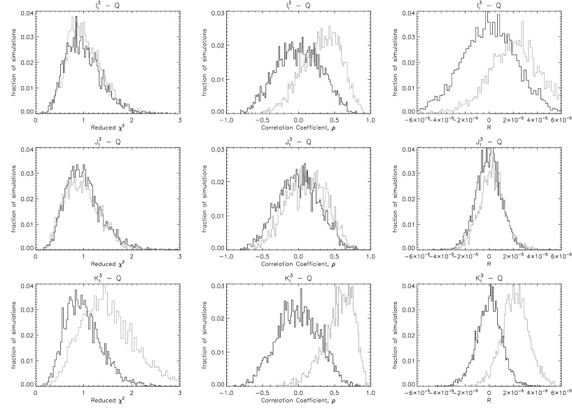
Figure 2: Distributions of values obtained for the three different tests applied to the Q channel to detect the presence of foregrounds ($\chi^{2}$, $\rho$ and ${\rm R}$), for Gaussian simulations (black) and contaminated ($\alpha=1.0$) simulations (grey). The level of sensitivity of a given method can be determined in terms of the shift between the histograms for the Gaussian and the contaminated case. We see that the $\rho^{K}$ and ${\rm R}^{K}$ statistics are the most sensitive channels to probe the existence of foregrounds.

Table 2: Results for the WMAP data for $\rho$ and ${\rm R}$. The results are shown as the fraction of Gaussian simulations below the level obseverved in the data. We have highlighted values with greater than 98% in the foreground cleaned maps.

	RAW			CLEANED
	${\rm Q}$	${\rm V}$	${\rm W}$	${\rm Q}$	${\rm V}$	${\rm W}$
${\rm R}^{I}$	0.726	0.178	0.328	0.475	0.421	0.775
${\rm R}^{J}$	0.758	0.802	0.749	0.822	0.869	0.983
${\rm R}^{K}$	0.983	0.450	0.486	0.362	0.364	0.188
$\rho^{I}$	0.998	0.408	0.762	0.491	0.550	0.452
$\rho^{J}$	0.933	0.906	0.856	0.998	0.985	0.986
$\rho^{K}$	0.922	0.166	0.272	0.013	0.021	0.044

5 Application to the WMAP data

We have applied the statistical tools described above to the WMAP first year data (Bennett et al., 2003a). We considered both the raw and cleaned maps of the Q, V, and W channels using the Kp2 exclusion mask. We summarise the results in table 2 showing the separate confidence limits from each channel for both the raw and cleaned maps.

For the raw maps we find that only the Q channel ${\rm R}^{K}$ result is above the 95% threshold while for the Q channel $\rho$ statistic, all confidence levels are above the 90% level with the $\rho^{I}$ above the 95% level. This is consistent with there being a component most correlated to the foreground templates at the lowest frequencies and with significant correlations between the $\Delta\ell=2$ inter-$\ell$ bispectrum and the power spectrum. Since the raw maps do not have any foreground subtracted from them this is not a surprise although the confidence level suggests that the correlations are larger than what was found for the expected amplitude ($\alpha=1$) of the foregrounds.

For all $I^{3}_{\ell}$ and $K^{3}_{\ell}$ statistics the cleaned map results show confidence levels below the 95% level and indeed show an overall reduction in the significance of the correlations, indicating that the cleaning has removed a component correlated to the foreground templates, as one would expect. However for the $J^{3}_{\ell}$ statistics, which should in principle be the least sensitive to the foregrounds considered, we see that the confidence levels have all increased. Indeed all three channels now have correlations significant above the 95% level in the $\rho$ statistic with the W channel also having a $>95\%$ confidence level. The cleaning algorithm appears to have introduced significant correlations with the foreground templates in the $\Delta\ell=1$ inter-$\ell$ bispectra and significant correlations between the $\Delta\ell=1$ inter-$\ell$ bispectrum and power spectrum of the W channel which is indicative of a non-Gaussian component.

In figure 3 we show the bispectra for each cleaned channel map and compare to the bispectra of the foreground template ($\alpha=1$) for each channel. This shows the nature of the result above. For both the $I^{3}_{\ell}$ and $K^{3}_{\ell}$ the cleaned map bispectra are anti-correlated with the foreground templates. In addition the the $K^{3}_{\ell}$ for all channels are heavily suppressed in the cleaned maps for multipoles $\ell<20$ compared to the expected Gaussian variance shown in figure 1. The $J^{3}_{\ell}$ gives the only bispectra that are correlated with the those of the templates.

Figure 4 shows the break down of the $R^{J}$ result into individual multipole contributions for each of the three bands. In particular it is interesting to note how the W band ${\rm R}^{J}$ result shown in table 2 is dominated by an outlier at $\ell=26$.

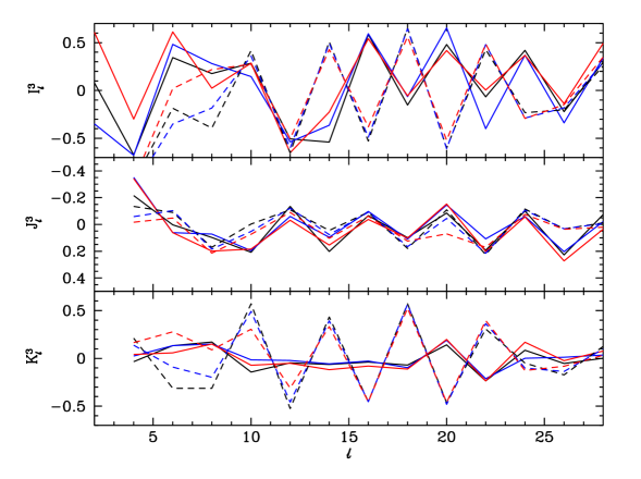
Figure 3: The bispectra for each cleaned channel map (solid line) against the bispectra of the foreground template ($\alpha=1.0$) (dashed lines). The three frequency channels are shown as Q (red), V (black) and W (blue). Both the cleaned map $I^{3}_{\ell}$ and $K^{3}_{\ell}$ bispectra are anti-correlated with the foreground templates. In addition the the $K^{3}_{\ell}$ for all channels are heavily suppressed in the cleaned maps for multipoles $\ell<20$ compared to the expected Gaussian variance shown in figure 1. The $J^{3}_{\ell}$ gives the only bispectra that are correlated with the those of the templates.

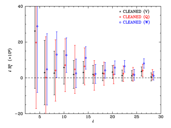
Figure 4: ${\rm R}^{J}$ as a function of angular scale, $\ell$. The values displayed correspond to the foreground cleaned Q (red squares), V (black triangles) and W (blue circles) frequency channels. The values are offset by $\ell=0.25$ and $\ell=0.5$ for the Q and W bands respectively. The $3\sigma$ detection in the W foreground-cleaned channel is dominated mainly by the $\ell=26$ mode. The error bars are computed from 3000 Gaussian simulations assuming the specific channel noise and beam.

6 Discussion

At first sight our results appear contradictory. We have studied the effect of foreground contamination on the maps and concluded that foregrounds mainly affect the $I^{3}_{\ell}$ and $K^{3}_{\ell}$ components of the bispectrum due to its parity. By comparing the results for the raw and the foreground-cleaned maps, we are able to verify that the amplitude of $I^{3}_{\ell}$ and $K^{3}_{\ell}$ reduces as expected after foreground subtraction.

On the other hand, as shown in table 2, the correlations induced in the $J^{3}_{\ell}$ appear to be close to inconsistent to a Gaussian hypothesis with the correlation with the foreground templates at a significance above the $3\sigma$ level for the Q-band, cleaned map. It is also of interest to note that the cleaned maps do worse in all bands for the $\rho$ measure.

This is not what we naively expected since the foregrounds considered here have the wrong parity and their $J^{3}_{\ell}$ signal is heavily suppressed. However the cleaning procedure used by the WMAP team does appear to increase the correlations $\rho$ of $J^{3}_{\ell}$ bispectrum to the input maps and its correlation $\rm R$ with the power spectrum. Recall that we expect the normalized bispectra to be independent of the power spectrum only in the Gaussian case.

The possibility of the foregrounds being more complex than accounted for in this type of treatment is to be considered carefully as this work has shown. The results shown here would suggest that the procedure used to go from the raw to cleaned WMAP maps is under or over subtracting a component with $\ell\pm 1$ parity in the bispectrum. This is probably not an indication that the procedure is faulty but rather that the templates used are not accurate enough to subtract the foregrounds. One source of inaccuracy is the simple scaling of the templates with respect to frequency. The cleaned maps are obtained assuming uniform spectral index and Bennett et al. (2003b) acknowledge that this is a bad approximation particularly for the 408 MHz Haslam (synchrotron) template. This is seen when producing the Internal Linear Combination (ILC) map which accounts for variation of the spectral index of the various component. Unfortunately ILC maps cannot be used in quantitative studies as their noise attributes are complicated by the fitting procedure and one cannot simulate them accurately.

Future WMAP ILC maps or equivalent ones obtained by ‘blind’ foreground subtraction (Tegmark et al., 2003; Eriksen et al., 2004b) may be better suited for this kind of analysis once their statistical properties are well determined. It is expected that the impending second release of WMAP data will allow more accurate foreground analysis and the statistical tools outlined in this work will be useful in determining the success of foreground subtraction.

It may be worthwile to include information of the higher order statistics when carrying out the foreground subtraction itself, for example by extending the ILC method to minimise higher order map quantities such as the skewness and kurtosis of the maps.

References

- Banday et al. (2000) Banday, A. J., Zaroubi, S., & Górski, K. M. 2000, ApJ, 533, 575
- Bennett et al. (1996) Bennett, C. L., et al. 1996, ApJ, 464, L1
- Bennett et al. (2003a) Bennett, C. L., et al. 2003, ApJS, 148, 1
- Bennett et al. (2003b) Bennett, C. L., et al. 2003, ApJS, 148, 97
- Bielewicz et al. (2004) Bielewicz, P., Górski, K. M., & Banday, A. J. 2004, MNRAS, 355, 1283
- Bridle et al. (2003) Bridle, S. L., Lewis, A. M., Weller, J., & Efstathiou, G. P. 2003, New Astronomy Review, 47, 787
- Coles et al. (2004) Coles, P., Dineen, P., Earl, J., & Wright, D. 2004, MNRAS, 350, 989
- Copi et al. (2004) Copi, C. J., Huterer, D., & Starkman, G. D. 2004, Phys. Rev. D, 70, 043515
- Contaldi et al. (2000) Contaldi, C. R., Ferreira, P. G., Magueijo, J., & Górski, K. M. 2000, ApJ, 534, 25
- Contaldi et al. (2003) Contaldi, C. R., Peloso, M., Kofman, L., & Linde, A. 2003, Journal of Cosmology and Astro-Particle Physics, 7, 2
- Efstathiou (2003) Efstathiou, G. 2003, MNRAS, 346, L26
- Eriksen et al. (2004a) Eriksen, H. K., Hansen, F. K., Banday, A. J., Górski, K. M., & Lilje, P. B. 2004, ApJ, 605, 14 [Erratum-ibid ApJ, 609, 1198]
- Eriksen et al. (2004b) Eriksen, H. K., Novikov, D. I., Lilje, P. B., Banday, A. J., & Górski, K. M. 2004, ApJ, 612, 633
- Eriksen et al. (2005) Eriksen, H. K., Banday, A. J., Górski, K. M., & Lilje, P. B. 2005, ApJ, 622, 58
- Ferreira & Magueijo (1997) Ferreira, P. G., & Magueijo, J. 1997, Phys. Rev. D, 56, 4578
- Ferreira et al. (1998) Ferreira, P. G., Magueijo, J., & Gorski, K. M. 1998, ApJ, 503, L1
- Finkbeiner (2003) Finkbeiner, D. P. 2003, ApJS, 146, 407
- Górski et al. (2005) Górski, K. M., Hivon, E., Banday, A. J., Wandelt, B. D., Hansen, F. K., Reinecke, M., & Bartelmann, M. 2005, ApJ, 622, 759
- Hansen et al. (2004) Hansen, F. K., Banday, A. J., & Górski, K. M. 2004, MNRAS, 354, 641
- Haslam et al. (1981) Haslam, C. G. T., Klein, U., Salter, C. J., Stoffel, H., Wilson, W. E., Cleary, M. N., Cooke, D. J., & Thomasson, P. 1981, A&A, 100, 209
- Land & Magueijo (2005) Land, K., & Magueijo, J. 2005, MNRAS, 357, 994
- Jaffe et al. (2005) Jaffe, T. R., Banday, A. J., Eriksen, H. K., Górski, K. M., & Hansen, F. K. 2005, ApJ, 629, L1
- Komatsu et al. (2002) Komatsu, E., Wandelt, B. D., Spergel, D. N., Banday, A. J., & Górski, K. M. 2002, ApJ, 566, 19
- Komatsu et al. (2003) Komatsu, E., et al. 2003, ApJS, 148, 119
- Komatsu, Spergel & Wandelt (2003) E. Komatsu, D. N. Spergel and B. D. Wandelt, background,” arXiv:astro-ph/0305189.
- Kogut et al. (1996) Kogut, A., Banday, A. J., Bennett, C. L., Gorski, K. M., Hinshaw, G., Smoot, G. F., & Wright, E. L. 1996, ApJ, 464, L29
- Larson & Wandelt (2004) Larson, D. L., & Wandelt, B. D. 2004, ApJ, 613, L85
- Magueijo (1995) Magueijo J., 1995, Phys. Lett, B342, 32. Erratum-ibid, B352, 499.
- Magueijo (2000) Magueijo, J. 2000, ApJ, 528, L57
- Magueijo & Medeiros (2004) Magueijo, J., & Medeiros, J. 2004, MNRAS, 351, L1
- Novikov, Feldman & Shandarin (1998) Novikov, D., Feldman, H. A. and Shandarin, S. F. 1999, Int. J. Mod. Phys. D 8, 291
- de Oliveira-Costa et al. (2004) de Oliveira-Costa, A., Tegmark, M., Zaldarriaga, M., & Hamilton, A. 2004, Phys. Rev. D, 69, 063516
- Pando et al. (1998) Pando, J., Valls-Gabaud, D., & Fang, L.-Z. 1998, Bulletin of the American Astronomical Society, 30, 1305
- Park (2004) Park, C.-G. 2004, MNRAS, 349, 313
- Peiris et al. (2003) Peiris, H. V., et al. 2003, ApJS, 148, 213
- Roukema et al. (2004) Roukema, B. F., Lew, B., Cechowska, M., Marecki, A., & Bajtlik, S. 2004, A&A, 423, 821
- Salopek et al. (1989) Salopek, D. S., Bond, J. R., & Bardeen, J. M. 1989, Phys. Rev. D, 40, 1753
- Sandvik & Magueijo (2001) Sandvik, H. B., & Magueijo, J. 2001, MNRAS, 325, 463
- Schwarz et al. (2004) Schwarz, D. J., Starkman, G. D., Huterer, D., & Copi, C. J. 2004, Physical Review Letters, 93, 221301
- Schlegel et al. (1998) Schlegel, D. J., Finkbeiner, D. P., & Davis, M. 1998, ApJ, 500, 525
- Slosar & Seljak (2004) Slosar, A., & Seljak, U. 2004, Phys. Rev. D, 70, 083002
- Tegmark et al. (2003) Tegmark, M., de Oliveira-Costa, A., & Hamilton, A. J. 2003, Phys. Rev. D, 68, 123523