Angular diameter distance estimates from the Sunyaev–Zeldovich effect in hydrodynamical cluster simulations

Abstract

The angular–diameter distance $D_{A}$ of a galaxy cluster can be measured by combining its X–ray emission with the cosmic microwave background fluctuation due to the Sunyaev–Zeldovich effect. The application of this distance indicator usually assumes that the cluster is spherically symmetric, the gas is distributed according to the isothermal $\beta$–model, and the X–ray temperature is an unbiased measure of the electron temperature. We test these assumptions with galaxy clusters extracted from an extended set of cosmological N-body/hydrodynamical simulations of a $\Lambda$CDM concordance cosmology, which include the effect of radiative cooling, star formation and energy feedback from supernovae. We find that, due to the temperature gradients which are present in the central regions of simulated clusters, the assumption of isothermal gas leads to a significant underestimate of $D_{A}$. This bias is efficiently corrected by using the polytropic version of the $\beta$–model to account for the presence of temperature gradients. In this case, once irregular clusters are removed, the correct value of $D_{A}$ is recovered with a $\sim 5$ per cent accuracy on average, with a $\sim 20$ per cent intrinsic scatter due to cluster asphericity. This result is valid when using either the electron temperature or a spectroscopic–like temperature. When using instead the emission–weighted definition for the temperature of the simulated clusters, $D_{A}$ is biased low by $\sim 20$ per cent. We discuss the implications of our results for an accurate determination of the Hubble constant $H_{0}$ and of the density parameter $\Omega_{m}$. We find that, at least in the case of ideal (i.e. noiseless) X-ray and SZ observations extended out to $r_{500}$, $H_{0}$ can be potentially recovered with exquisite precision, while the resulting estimate of $\Omega_{m}$, which is unbiased, has typical errors $\Delta\Omega_{m}\simeq 0.05$.

1 Introduction

The Sunyaev–Zeldovich (SZ) effect (Sunyaev & Zeldovich, 1972) is the distortion of the Cosmic Microwave Background (CMB) spectrum due to the scattering of the CMB photons off a population of electrons. At radio frequencies, the typical size of this distortion for a thermal distribution of electrons with temperature of about 10 keV is at the level of $10^{-4}$. This effect has now been detected for a fairly large number of clusters of galaxies (e.g. Rephaeli, 1995; Birkinshaw, 1999; Carlstrom et al., 2002, for reviews). For almost three decades it has been recognized that the combination of X–ray and SZ observations of galaxy clusters provides a direct measurement of the cosmic distance scale, under the assumption of spherical symmetry for the intra–cluster gas distribution (e.g. Gunn, 1978; Silk & White, 1978; Cavaliere et al., 1979; Birkinshaw, 1979). The method is based on the different dependence on the electron number density, $n_{e}$, of the X–ray emissivity ($\propto n_{e}^{2}T_{e}^{1/2}$ for thermal bremsstrahlung; here $T_{e}$ is the electron temperature) and of the SZ signal ($\propto n_{e}T_{e}$).

Due to the crucial role played by the assumption of spherical symmetry, a great deal of efforts have been spent either to select individual clusters having very relaxed and regular morphology (e.g. Holzapfel et al., 1997; Hughes & Birkinshaw, 1998; Grainge et al., 2002; Bonamente et al., 2004), or to build suitable cluster samples over which averaging out the uncertainties due to intrinsic cluster ellipticity (e.g. Mason et al., 2001; Reese et al., 2002; Udomprasert et al., 2004; Jones et al., 2005). These analyses have provided estimates of the Hubble constant, $H_{0}$, which are generally consistent with those obtained from the Cepheid distance scale (e.g. Freedman et al., 2001) or inferred from the spectrum of the CMB anisotropies (e.g. Spergel et al., 2003), although with fairly large uncertainties. Although the dominant source of uncertainty is probably represented by the contamination of the SZ signal by the CMB and point–sources (e.g. Udomprasert et al., 2004), significant errors are also associated to cluster asphericity, clumpy gas distribution and incorrect modeling of the thermal structure of the intra–cluster medium (ICM).

So far, the limited number of high–redshift clusters with both SZ and X–ray observations, with their relatively large uncertainties, made the calibration of the cosmic distance scale mostly sensitive to the value of $H_{0}$, while no significant constraints have been placed on the values of the matter density parameter $\Omega_{m}$ and the cosmological constant. In the coming years, ongoing X–ray (e.g., Mullis et al., 2005), optical (e.g., Gladders & Yee, 2005), and planned or just started SZ surveys promise to largely increase the number of observed clusters out to $z\sim 1.5$. This may well open the possibility to use SZ/X–ray cluster observations to place constraints on the Dark Matter and Dark Energy content of the universe (Molnar et al., 2002). This highlights the paramount importance of having observational uncertainties under control.

In this respect, numerical hydrodynamical simulations of galaxy clusters may offer an important test–bed where to quantify observational biases and keep the corresponding uncertainties under control. For instance, eliminating $n_{e}$ from the SZ and X–ray signal leaves a sensitive dependence of the angular–diameter distance, $D_{A}$, on the electron temperature (see §2). On the other hand, temperature measurements of the ICM have been so far entirely based on fitting the X–ray spectrum to a suitable plasma model. How close is the resulting spectral temperature to the electron temperature depends on the complexity of the thermal structure of the ICM (e.g., Mazzotta et al., 2004). Hydrodynamical simulations of clusters offer a natural way to quantify the bias introduced by replacing the electron temperature with the X–ray temperature. Furthermore, the standard assumption in the SZ/X–ray calibration of the cosmic distance scale is that of the isothermal ICM, while X–ray observations of clusters clearly show the presence of significant temperature gradients (e.g. Markevitch et al., 1998; De Grandi & Molendi, 2002; Vikhlinin et al., 2005). To overcome this problem, several authors estimate the bias introduced by the isothermal approximation, finding that the distance can be biased by $\raise-2.0pt\hbox{\hbox to0.0pt{\hbox{$\sim$}\hss}\raise 5.0pt\hbox{$<$}\ }20$ per cent (e.g. Birkinshaw & Hughes, 1994; Udomprasert et al., 2004; Holzapfel et al., 1997). Simulations of galaxy clusters naturally produce temperature gradients that, at least at large radii, are close to the observed ones (e.g., Loken et al., 2002; Borgani et al., 2004; Kay et al., 2004). Therefore, simulations can be used to quantify the bias introduced by the assumption of isothermal gas. Finally, using a representative set of galaxy clusters in a cosmological framework allows one to trace the distribution of ellipticity and, therefore, to calibrate the corresponding scatter in the measurement of the distance scale. Nowadays, cosmological hydrodynamical codes have reached a high enough efficiency, in terms of both achievable resolution and description of the gas physics, to provide a realistic description of the processes of formation and evolution of galaxy clusters (e.g. Borgani et al., 2004; Kravtsov et al., 2005). For instance, Kazantzidis et al. (2004) found that halos in hydrodynamical simulations including cooling are significantly more spherical than in non–radiative simulations. Since the assumption of sphericity is at the basis of the X–ray/SZ method to estimate $D_{A}$, this highlights the relevance of properly modeling the physics of the ICM for a precise calibration of the cosmic distance scale.

The purpose of this paper is to understand the impact of the above discussed systematics on the calibrations of the cosmic distance scale from the combination of SZ and X–ray observations, by analyzing an extended set of hydrodynamical simulations of galaxy clusters. These simulations have been performed using the TREE+SPH GADGET–2 code (Springel et al., 2001; Springel, 2005), for a concordance $\Lambda$CDM model, and include the processes of radiative cooling, star formation and supernova feedback. The set of simulated clusters contains more than 100 objects having virial masses in the range $(2-20)\times 10^{14}h^{-1}M_{\odot}$.

The plan of the paper is as follows. In Section 2 we review the method to estimate the angular–diameter distance from X–ray and SZ cluster observations in the case of a polytropic equation of state for the ICM, and discuss the different definitions of temperature that are used in the analysis of the simulations. In Section 3 we describe the set of simulated clusters and the procedure to generate X–ray and SZ maps. We present our results in Section 4, where we show the results on the accuracy of the measurement of $D_{A}$. We discuss and summarize our main results in Section 5.

2 $D_{A}$ from combined X-ray and SZ observations

The combination of the ICM X-ray emission with the SZ flux decrement provides a direct measure of the angular-diameter distance, $D_{A}$, of galaxy clusters (Silk & White, 1978; Cavaliere et al., 1979; Birkinshaw, 1979). The method takes advantage of the different dependences of these two quantities on the electron number density, $n_{e}$ (the former is $\propto n_{e}^{2}$ while the latter is $\propto n_{e}$). When combined, these two quantities provide the physical dimension of the cluster along the line-of-sight and, from the cluster angular size, $D_{A}$, if the cluster is spherically symmetric.

The Comptonization parameter $y$, as measurable from observations of the SZ effect, is

$$y=\int n_{e}\frac{k_{B}T_{e}}{m_{e}c^{2}}\sigma_{T}d\ell$$ (1)

where $k_{B}$ is the Boltzmann constant, $\sigma_{T}$ is the Thompson cross section, $m_{e}$ is the mass of the electron, $c$ is the speed of light and the integration is along the line of sight. By definition, it provides a redshift–independent measure of the total thermal content of the cluster.

The X-ray surface brightness $S_{X}$ is

$$S_{X}=\frac{1}{4\pi(1+z)^{4}}\int n_{e}n_{H}\Lambda_{eH}(T)d\ell$$ (2)

where $n_{H}$ is the hydrogen number density of the ICM, $\Lambda_{eH}(T)$ is the cooling function (normalized to $n_{e}n_{H}$). To compute the X–ray emissivity of the simulated clusters, we assume the cooling function taken from a Raymond-Smith code (Raymond & Smith, 1977) for a gas of primordial composition ($X_{H}=0.76$ and $X_{He}=0.24$) for a fully ionized ICM. We compute the X–ray emissivity in the [0.5–2] keV energy band, which is used in several combined SZ/X–ray analyses relying on the ROSAT–PSPC data for the X–ray imaging part (e.g. Reese et al., 2002; Jones et al., 2005). Using bands extending to higher energies, as appropriate for Chandra and XMM–Newton observations, would produce no change in the final results.

2.1 The polytropic $\beta$–model

A common procedure adopted to extract $D_{A}$ from the combination of eqs. (1) and (2) is based on modeling the electron density profile with the $\beta$-model,

$$n_{e}(r)=n_{e0}\left[1+\left(\frac{r}{r_{c}}\right)^{2}\right]^{-3\beta/2}$$ (3)

(Cavaliere & Fusco-Femiano, 1976), where $n_{e0}$ is the electron number density in the cluster center, $r$ is the distance from the cluster center, $r_{c}$ is the core radius and $\beta$ is the power–law index.

As for the temperature structure of the ICM, a number of analyses of X–ray data independently show that galaxy clusters are far from being isothermal. Significant negative gradients characterize the temperature profiles of galaxy clusters, at least on scales $R\raise-2.0pt\hbox{\hbox to0.0pt{\hbox{$\sim$}\hss}\raise 5.0pt\hbox{$>$}\ }0.2R_{200}$ (e.g. Markevitch et al., 1998; De Grandi & Molendi, 2002; Pratt & Arnaud, 2002; Piffaretti et al., 2005; Vikhlinin et al., 2005), with positive gradients associated only to the innermost cooling regions (e.g. Allen et al., 2001). The dynamic range covered by the SZ signal extends on scales which are relatively larger than those sampled by the X–ray emission. For this reason, one may expect that a systematic effect is introduced by assuming the ICM to be isothermal when combining X–ray and SZ observations. Since the SZ signal has a stronger dependence on the ICM temperature than the X–ray one, the effect of assuming an isothermal ICM, in a regime where the temperature is decreasing, may lead to predict $y(\theta)$–profiles which are shallower than the intrinsic ones.

In order to account for the presence of temperature gradients, we introduce a polytropic equation of state, $p\propto\rho^{\gamma}$, which relates the gas pressure $p$ to the density $\rho$, where $\gamma$ is the polytropic index ($\gamma=1$ for isothermal gas). The three-dimensional temperature profile is thus

$$T_{e}(r)=T_{e0}\left(n_{e}\over n_{e0}\right)^{\gamma-1}=T_{e0}\left[1+\left(\frac{r}{r_{c}}\right)^{2}\right]^{-3\beta(\gamma-1)/2},$$ (4)

where $T_{e0}$ is the temperature at the cluster center. Using the above expression for the temperature profile in the definition of the Comptonization parameter of eq.(1) gives

$$y(\theta)=y_{0}\left[1+\left(\frac{\theta}{\theta_{c}}\right)^{2}\right]^{(1-3\beta\gamma)/2}\,,$$ (5)

where the Comptonization parameter at the cluster center is

$$y_{0}=D_{A}n_{e0}\theta_{c}\sigma_{T}{k_{B}T_{e0}\over m_{e}c^{2}}\sqrt{\pi}{\Gamma(3\beta\gamma/2-1/2)\over\Gamma(3\beta\gamma/2)}\,.$$ (6)

Similarly, we obtain the X–ray surface brightness profile

$$S_{X}(\theta)=S_{X0}\left[1+\left(\frac{\theta}{\theta_{c}}\right)^{2}\right]^{\left\{1-6\beta[(\gamma+3)/4]\right\}/2}\,,$$ (7)

where the central surface brightness is

$$S_{X0}=D_{A}n_{e0}^{2}\theta_{c}{1\over 4\sqrt{\pi}}{\mu_{e}\over\mu_{H}}\Lambda_{eH}(T_{e0}){\Gamma(3\beta[(\gamma+3)/4]-1/2)\over\Gamma(3\beta[(\gamma+3)/4]}\,.$$ (8)

In deriving the above equation, the dependence of the cooling function on $T_{e}$ is assumed to be a power law, $T^{\alpha}$, with index $\alpha=0.5$. This is valid in the case of pure bremsstrahlung emission and represents a good approximation in the case of bolometric emissivity. However, our emissivity maps are build in the [0.5-2] keV band. In this energy range the cooling function is significantly flatter, due to the contribution of metal emission lines, which is relevant in the case of relatively cool systems ($T_{e}<2$ keV) (e.g. Ettori, 2000). In order to test the effect of approximating the cooling function with a bremsstrahlung shape, we repeated our analysis also in the bolometric band and found variations in the final distance estimates by $\raise-2.0pt\hbox{\hbox to0.0pt{\hbox{$\sim$}\hss}\raise 5.0pt\hbox{$<$}\ }10\%$.

Finally, by eliminating $n_{e0}$ from eqs.(6) and (8), we obtain the angular–diameter distance

$$D_{A} = \frac{y_{0}^{2}}{S_{X0}}\left[\frac{m_{e}c^{2}}{k_{B}T_{e0}}\right]^{2}\frac{\Lambda_{eH}(T_{e0})\mu_{e}/\mu_{H}}{4\pi^{3/2}\sigma_{T}^{2}(1+z)^{4}}\frac{1}{\theta_{c}}$$ (9)

$$\times\left[\frac{\Gamma(3\beta\gamma/2)}{\Gamma(3\beta/2-1/2)}\right]^{2}\frac{\Gamma(3\beta[(\gamma+3)/4]-1/2)}{\Gamma(3\beta[(\gamma+3)/4])}\,.$$

For $\gamma=1$, the above expression reduces to that usually adopted in observational analyses based on combining X–ray and SZ cluster observations (e.g. Reese et al., 2002; Udomprasert et al., 2004; Bonamente et al., 2004), which relies on the assumption of isothermal gas.

It is worth reminding here that, while simulations are rather successful in reproducing the negative temperature gradient in the outer cluster regions (e.g. Evrard et al., 1996; Eke et al., 1998; Loken et al., 2002; Rasia et al., 2004), they generally produce too steep profiles in the central cluster regions, especially when radiative cooling is included (e.g. Katz & White, 1993; Tornatore et al., 2003; Valdarnini, 2003; Borgani et al., 2004). Since observed clusters are characterized by a core region which is closer to isothermality than the simulated ones, we expect that the effect of using a polytropic temperature profile when analyzing simulated clusters is larger than the actual effect taking place in real clusters.

2.2 Definitions of temperature

In the observational determinations of $D_{A}$ from X–ray and SZ observations with eq.(9) one relies on the X–ray temperature obtained from the spectral fitting. Such a spectral temperature is generally different from both the actual electron temperature, which appears in the expression of $D_{A}$, and the emission–weighted temperature, which is often used as a proxy to the spectral temperature in the analysis of hydrodynamical simulations of clusters (e.g. Evrard et al., 1996).

If $n_{e,i}$ and $T_{i}$ are defined as the electron number density and the temperature carried by the $i$–th simulation gas particle, then the electron temperature is defined by

$$T_{e}=\sum_{i}n_{e,i}T_{i}/\sum_{i}n_{e,i}\,,$$ (10)

which coincides with the mass–weighted temperature in the limit of a fully ionized plasma of uniform metallicity. Analogously, the emission–weighted temperature is

$$T_{ew}={\sum_{i}\Lambda(T_{i})n_{e,i}^{2}T_{i}\over\sum_{i}\Lambda(T_{i})n_{e,i}^{2}}\,,$$ (11)

where the cooling function $\Lambda(T)$ can be computed over an energy band, comparable to that where the X–ray spectrum is fitted in observational data analyses. In the following, we compute the emissivity in the [0.5–7] keV band.

However, Mathiesen & Evrard (2001) were the first to show that the emission–weighted temperature does not necessarily represent an accurate approximation to the spectroscopic temperature. Mazzotta et al. (2004) have further motivated and quantified this difference, connecting it to a thermally complex structure of the ICM. These authors suggested an approximate expression for the spectroscopic temperature, the spectroscopic–like temperature:

$$T_{sl}=\frac{\sum_{i}n_{e,i}^{2}T_{i}^{a+1/2}}{\sum_{i}n_{e,i}^{2}T_{i}^{a+3/2}}\,,$$ (12)

where $a$ is a fitting parameter. Mazzotta et al. (2004) have shown that eq.(12) with $a=0.75$ closely reproduces the spectroscopic temperature of clusters at least as hot as 3 keV, with a few per cent accuracy, after excluding all the gas particles colder than 0.5 keV from the sums in eq.(12). More recently, (Vikhlinin, 2005) has generalized the above expression for $T_{sl}$ to include the cases of lower temperatures and arbitrary ICM metallicity.

In the following, besides using the electron temperature, we also perform our analysis by relying on the temperature proxies of eqs.(11) and (12). Therefore, comparing the results based on the electron temperature and on the spectroscopic–like temperature provides a check of the bias introduced by using the X–ray temperature in the estimate of $D_{A}$, a bias possibly present also in the analysis of real data. Furthermore, the comparison between emission–weighted and spectroscopic–like temperature provides a hint on the bias introduced in the simulation analysis when using an inaccurate proxy to the X–ray temperature. It is worth reminding here that, due to the finite time for electron–ion thermalization, the corresponding electron and ion temperature may differ, for instance as a consequence of continuous shocks (e.g., Yoshida et al., 2005). A sizable difference among these two temperatures may induce a bias in the estimate of the distance scale.

Except for using different definitions of temperature, we do not investigate the effect of a realistic observational setup for the detection of both the SZ and X–ray signals. Besides the statistical errors associated to time–limited exposures, we also neglect the effects of systematics (e.g., instrumental noise, foreground and background contribution from contaminants, etc.). A detailed analysis of the contaminations in the SZ signal has been provided by Knox et al. (2004) and by Aghanim et al. (2004). A comprehensive description of the instrumental effects on the recovery of X–ray observables, calibrated on hydrodynamical simulations, has been provided by Gardini et al. (2004) (see also Rasia et al., 2006). In this sense, our analysis will be based on ideal maps, which are free of any noise. We defer to a future analysis the inclusion of the errors associated to realistic X–ray and SZ observational setups.

3 The simulated clusters

The sample of simulated galaxy clusters used in this paper has been extracted from the large-scale cosmological hydro-N-body simulation of a “concordance” $\Lambda$CDM model with $\Omega_{m}=0.3$ for the matter density parameter at present time, $\Omega_{\Lambda}=0.7$ for the cosmological constant term, $\Omega_{\rm b}=0.019\,h^{-2}$ for the baryons density parameter, $h=0.7$ for the Hubble constant in units of 100 km s^-1Mpc^-1 and $\sigma_{8}=0.8$ for the r.m.s. density perturbation within a top–hat sphere having comoving radius of $8\,h^{-1}{\rm Mpc}$. We refer to Borgani et al. (2004) (B04 hereafter) for a detailed presentation of this simulation, while we give here only a short description.

The run, performed with the massively parallel Tree+SPH code GADGET-2 (Springel et al., 2001; Springel, 2005), follows the evolution of $480^{3}$ dark matter particles and an equal number of gas particles in a periodic cube of size $192h^{-1}$ Mpc. The mass of the gas particles is $m_{\rm gas}=6.9\times 10^{8}h^{-1}M_{\odot}$, while the Plummer-equivalent force softening is $7.5h^{-1}$ kpc at $z=0$. Besides gravity and hydrodynamics, the simulation includes the treatment of radiative cooling, the effect of a uniform time–dependent UV background, a sub–resolution model for star formation from a multiphase interstellar medium, as well as galactic winds powered by SN explosions (Springel & Hernquist, 2003). At $z=0$ we extract a set of 117 clusters, whose mass, as computed from a friends-of-friends algorithm with linking length $b=0.15$ (in units of the mean interparticle distance) is larger than $10^{14}\,h^{-1}M_{\odot}$.

Due to the finite box size, the largest cluster found in the cosmological simulation has $T_{\rm e}\approx 5$ keV. In order to extend our analysis to more massive and hotter systems, which are mostly relevant for current SZ observations, we include four more galaxy clusters having $M_{\rm vir}>10^{15}\,h^{-1}M_{\odot}$ and belonging to a different set of hydro-N-body simulations (Borgani et al., 2006). Since these objects have been obtained by re-simulating, at high resolution, a patch of a pre-existing cosmological simulation, they have a better mass resolution, with $m_{\rm gas}=1.69\times 10^{8}h^{-1}M_{\odot}$. These simulations have been performed by using the same code with the same choice of the parameters defining star–formation and feedback. The cosmological parameters also are the same, except for a larger power spectrum normalization, $\sigma_{8}=0.9$.

Therefore, our total sample comprises 121 objects, spanning the range of spectroscopic temperatures $T_{sl}\simeq 1-9$ keV, out of which 25 have $T_{sl}>2.5$ keV and only four have $T_{sl}>5$ keV. The corresponding temperature distribution is reported in Figure 1. Quite apparently, our set of clusters on average samples a lower temperature range with respect to that covered by current SZ observations. For this reason, we will discuss in the following the stability of our results when selecting only the high end of the temperature distribution. Since our set of simulated clusters covers a relatively low temperature range, we can safely ignore any relativistic corrections to the SZ signal (e.g., Itoh et al., 1998).

Figure 1: The distribution of spectroscopic–like temperatures for the set of simulated clusters. The dashed and the solid lines are for the whole sample and for the subset of clusters classified as regular (see text), respectively.

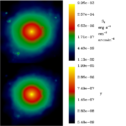
Figure 2: Maps of the X-ray brightness and SZ $y$ parameter for a regular simulated cluster having virial mass $M_{vir}\simeq 1.4\cdot 10^{14}h^{-1}M_{\odot}$, $R_{500}=0.53h^{-1}Mps$ and $T_{sl}=2.2$ keV. The map extends out to 2 $R_{\rm vir}$, so that it covers a physical scale of 6.05 $\,h^{-1}{\rm Mpc}$ for this cluster. Each map is done with a $256\times 256$ pixelization.

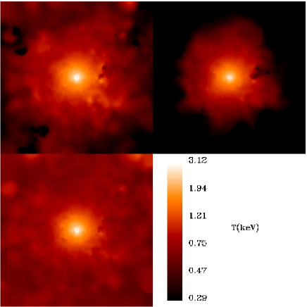
Figure 3: Maps of the emission-weighted (top left), mass-weighted (top right) and spectroscopic-like (bottom left) temperature for the same cluster of Figure 2.

Around each cluster we extract a spherical region extending out to 6 $R_{vir}$. Following Diaferio et al. (2005), we create maps of the relevant quantities along three orthogonal directions, extending out to about 2 $R_{vir}$ from the cluster center. Each map is a regular $256\times 256$ grid.

In the Tree+SPH code, each gas particle has a smoothing length $h_{i}$ and the thermodynamical quantities it carries are distributed within the sphere of radius $h_{i}$ according to the compact kernel:

$$W(x)=\frac{8}{\pi h_{i}^{3}}\left\{\begin{array}[]{ll}1-6x^{2}+6x^{3}&0\leq x\leq\frac{1}{2}\\ 2(1-x)^{3}&\frac{1}{2}\leq x\leq 1\\ 0&x\geq 1\end{array}\right.$$ (13)

where $x=r/h_{i}$ and $r$ is the distance from the particle position. We therefore distribute the quantity of each particle on the grid points within the circle of radius $h_{i}$ centered on the particle. Specifically, we compute a generic quantity $q_{jk}$ on the $(j,k)$ grid point as $q_{jk}d^{2}_{p}=\int q(r)dld^{2}_{p}=\sum q_{i}(m_{i}/\rho_{i})w_{i}$ where $d^{2}_{p}$ is the pixel area, the sum runs over all the particles, and $w_{i}\propto\int W(x)dl$ is the weight proportional to the fraction of the particle proper volume $m_{i}/\rho_{i}$ which contributes to the $(j,k)$ grid point. For each particle, the weights $w_{k}$ are normalized to satisfy the relation $\sum w_{k}=1$ where the sum is now over the grid points within the particle circle. When $h_{i}$ is so small that the circle contains no grid point, the particle quantity is fully assigned to the closest grid point. Figures 2 and 3 show an example of the X-ray surface brightness and SZ maps and of the temperature maps of a relaxed cluster in our simulation (with $M_{vir}\simeq 1.4\cdot 10^{14}h^{-1}M_{\odot}$), which we use in the following as an example.

4 Results

In this section we present our results on the reliability of the usual procedure to recover the angular–diameter distance from the combination of the SZ and X–ray emission of clusters, by using both the isothermal and a more general polytropic equation of state for the ICM. Since the procedure to determine $D_{A}(z)$ is known to be particularly sensitive to the presence of cluster substructures and irregularities, the first step of our analysis is to select a subset of relaxed and regular clusters. Our selection criterion is based on visual inspection of the X–ray and SZ maps, as well as on the profiles of the X–ray surface brightness and the Comptonization parameter. Although this is clearly not an objective criterion, it is quite similar to the criteria used to classify real clusters. Besides the example of a relaxed cluster shown in Figure 2, in Figure 4 we also show an example of a cluster that we classify as unrelaxed and, as such, is excluded from our analysis. Overall, we select 71 relaxed clusters from the initial sample of 121 simulated clusters (the four hottest clusters are all included in this subset). The temperature distribution of these objects is represented in figure 1 with a solid line. We have 19 clusters in this subset with $T_{sl}>2.5$ keV. We extend our statistical sample by realizing “observations” of each cluster along three orthogonal lines of sight and treating them as three independent objects.

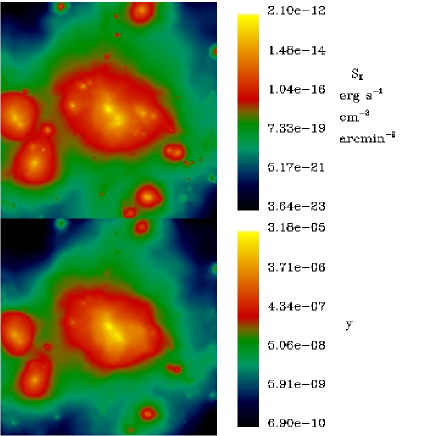
Figure 4: The same as Fig.2, but for an unrelaxed simulated cluster having virial mass $M_{vir}\simeq 4.1\cdot h^{-1}10^{14}M_{\odot}$.

4.1 Results from the isothermal model

Unlike X–ray observations, current observations of the SZ effect in clusters do not allow to perform any spatially resolved analysis. For this reason, the commonly adopted procedure is to determine the parameters $\theta_{c}$ and $\beta$, which determined the $\beta$–model density profile, from the X-ray imaging alone, along with the normalization $S_{X0}$. The SZ profile is then used to obtain the central value of the Comptonization parameter, $y_{0}$, by using the $\beta$-model parameters as determined from the X-ray profile. By following this procedure, we fitted all the profiles out to $R_{500}$, which is defined as the radius encompassing an average density of 500 times the critical cosmic density. We point out that $R_{500}$ corresponds to the typical outermost radius where X-ray observations provide surface brightness and temperature profiles. We exclude from the analysis the central regions of the clusters, within $1/20R_{\rm vir}$, which are strongly affected by gas cooling and are close to the numerical resolution of the simulations.

In Figure 5 we show the profiles of the X–ray surface brightness and Compton–$y$ for the example cluster of Fig.2, along with the best–fitting $\beta$–model for the isothermal case. For this relaxed cluster, the $\beta$–model provides a rather good fit to the X-ray profile. Only the central point, which is anyway excluded from the fit, is higher than the $\beta$–model extrapolation, as a consequence of the high–density gas residing in the cluster cooling region. The resulting values of the fitting parameters for this cluster are $\beta=0.835$ and $r_{c}/R_{500}=0.196$. Fitting the $y(R)$ profile with eq.(5), after setting $\beta=0.835$ and $\gamma=1$, leads to an underestimate of $y_{0}$. In fact, the resulting Compton–$y$ profile is significantly shallower than measured (Figure 5). This result follows from neglecting the presence of negative temperature gradients. Consequently we tend to underestimate $D_{A}$, because $D_{A}\propto y_{0}^{2}$ [see eq.(9)]. In this particular case we underestimate $D_{A}$ by 56 per cent.

Figure 5: The projected radial profiles of $X$–ray surface brightness (left panel) and of Compton–$y$ parameter (right panel) for the cluster shown in Fig.2. Symbols are for the results of the simulation analysis while the solid curves are the predictions of the isothermal $\beta$–model.

This result for one particular cluster is confirmed by the distribution shown in the left panel of Figure 6 (see also Table 1). In this figure we report the distribution of the ratios $D_{A}^{\rm rec}/D_{A}^{\rm true}$ between the recovered and the true values of the angular–size distance. Such results clearly demonstrate that the angular–size distance is biased low, on average, by more than a factor two, as a consequence of the underestimate of $y_{0}$ induced by the assumption of an isothermal ICM. In order to verify a possible temperature dependence of the $D_{A}$ distribution, in the left panel of Fig.6 we also show the results for the clusters with $T_{sl}$ in the range 2.5–5 keV and for those hotter than 5 keV. While the latter are too few to allow any meaningful conclusion, the clusters at intermediate temperature have a distribution which is statistically consistent with that of the whole sample. This indicates the absence of any obvious trend of our results with the cluster size. The results reported in this figure have been obtained by using the electron–weighted temperature estimate for the simulated clusters. If we had used the emission–weighted temperature, we would have obtained an even stronger bias (see eq.[9]), because this temperature generally overestimates the electron temperature.

Including dynamically disturbed clusters does not significantly affect the average value of the recovered $D_{A}$. However, the resulting distribution is clearly asymmetric and presents a large tail towards low $D_{A}$ values. In fact, eqs. (1) and (2) show that that $D_{A}\propto\langle n_{e}\rangle^{2}/\langle n_{e}^{2}\rangle$. Therefore, the presence of clumps in the gas distribution produces an underestimate of $D_{A}$ by this factor with respect to a completely smooth gas distribution. By looking at the distributions of the $\beta$ and $r_{c}$ (central and left panels of Fig.6), unrelaxed structures tend to have rather flat gas density profiles. Fitting them with a $\beta$–model forces the slope to be very small, with a preference for the core radius to be consistent with zero. For instance, the cluster shown in Fig.4 requires $\beta=0.52$ and $r_{c}/R_{500}=0.03$, while its estimate of the angular–size distance gives $D_{A}^{\rm rec}/D_{A}^{\rm true}=0.17$.

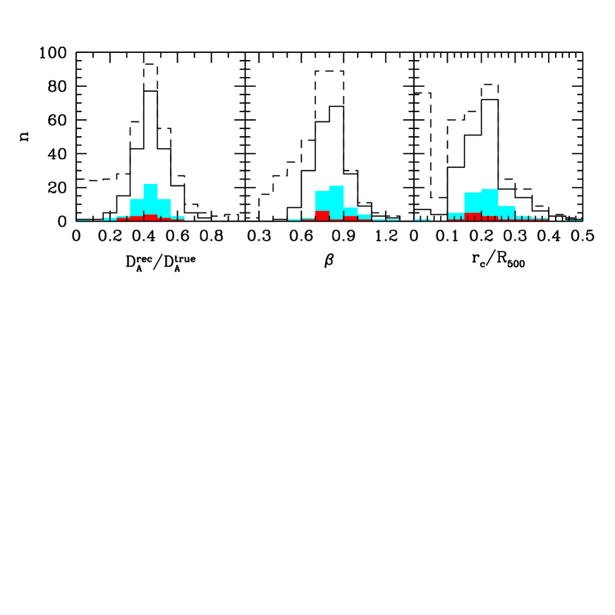
Figure 6: The distribution of the values of $D_{A}^{rec}/D_{A}^{true}$ (left panel), of $\beta$ (central panel) and of $r_{c}$ (in units of $R_{500}$; right panel). The dashed and the solid lines are respectively for the whole sample and for the subset of clusters classified as regular. Also shown with the light and dark gray areas are the corresponding distributions for the subset of the clusters with $2.5<T_{sl}(keV)<5$ and $T_{sl}(keV)>5$, respectively. classified as regular. The distribution of $D_{A}^{rec}/D_{A}^{true}$ is obtained by using the electron–weighted temperatures of the simulated clusters in eq.(9).

As a word of caution in interpreting such results, we emphasize that this bias in the $D_{A}$ estimate, due to the isothermal gas assumption, is likely to represent an overestimate of the actual effect in real cluster observations for at least two reasons. First, radiative simulations of clusters are known to produce temperature gradients that, in the central regions, are steeper than observed (see the discussion in §2.1). As a consequence, simulated clusters exaggerate the departure from isothermality. Second, the $\beta$–model fitting to the Compton–$y$ profile has been performed by assigning equal weight to all radial bins, with the more external regions bringing down the overall normalization of the model profile. In a realistic observational setup, the signal from central cluster regions should have a relatively larger weight, thus reducing the bias in the recovered $y_{0}$. Addressing appropriately this issue would require implementing detailed mock SZ observations of our simulated clusters, a task that we defer to a future analyses. Even keeping in mind these warnings, it is clear that deviations from isothermality must be taken into account for a precise calibration of the cosmic distance scale from the combination of X–ray and SZ observations of galaxy clusters (e.g., Udomprasert et al., 2004).

	All	Regular
	clusters	clusters
Isothermal	$0.41\pm 0.27$	$0.44\pm 0.11$
	$0.42_{-0.22}^{+0.14}$	$0.45_{-0.10}^{+0.10}$
Polytropic
$T_{ew}$	$0.76\pm 0.74$	$0.80\pm 0.15$
	$0.78_{-0.37}^{+0.19}$	$0.81_{-0.17}^{+0.14}$
$T_{e}$	$0.95\pm 0.49$	$1.04\pm 0.22$
	$0.98_{-0.47}^{+0.31}$	$1.05_{-0.26}^{+0.21}$
$T_{sl}$	$0.99\pm 2.57$	$0.97\pm 0.18$
	$0.92_{-0.46}^{+0.25}$	$0.98_{-0.20}^{+0.18}$

Table 1: The values of the accuracy in recovering the angular–diameter distance, $D_{A}^{\rm rec}/D_{A}^{\rm true}$, using both the isothermal and the polytropic model, and using the emission–weighted, the electron and the spectroscopic–like definitions of temperature. For each of them, the first line reports the mean and standard deviation, the second the median and the limiting values encompassing 68% of the data.

4.2 Results from the polytropic fit

In the case of a more general polytropic equation of state, the parameters $\beta$ and $\gamma$ are calculated by requiring the model to reproduce at the same time both the X-ray surface brightness and the temperature profiles. After obtaining the core radius $r_{c}$ and the normalization $S_{X0}$ from the X-ray profile, and $T_{0}$ from the temperature profile, we combine the two exponents in eqs. (7) and (4) to derive both $\beta$ and $\gamma$, with $y_{0}$ finally obtained from the SZ profile.

Figure 7: Profiles of temperature (upper panels) and of Compton–$y$ parameter (lower panels) for the cluster of Fig.2. Left, central and right panels corresponds to using emission–weighted, electron and spectroscopic–like temperature, respectively. Open symbols are for the profiles from the simulation analysis, while the curves are the best–fitting polytropic $\beta$–model.

In Figure 7 we show the temperature and Compton–$y$ profiles for our example cluster, along with the best–fitting predictions of the polytropic $\beta$–model, for the three different definitions of temperature. The polytropic equation of state provides a reasonable approximation to all temperature profiles and, unlike the isothermal case, allows us to correctly predict also the Compton–$y$ profile. The corresponding distributions of $\beta$ and $\gamma$ are shown in Figure 8 (we do not report the distribution of $r_{c}$, since it is, by definition, identical to that of the isothermal model). For both quantities, the effect of using different definitions of temperature is rather small. As expected, using a polytropic temperature profile implies only a modest decrease of the $\beta$ values, because of the weak temperature dependence of the cooling function. All the three distributions of $\gamma$ have an average value $\simeq 1.2$, similar to observational estimates (e.g. De Grandi & Molendi, 2002). Moreover, the scatter in this distribution is so small to make the isothermal ICM an extremely unlikely event.

Figure 8: Distributions of the values of $\beta$ (left panel) and $\gamma$ (right panel), using emission–weighted (solid line), electron (dotted line) and spectroscopic–like (dashed lines) temperatures, respectively, as obtained for the whole sample of 121 clusters.

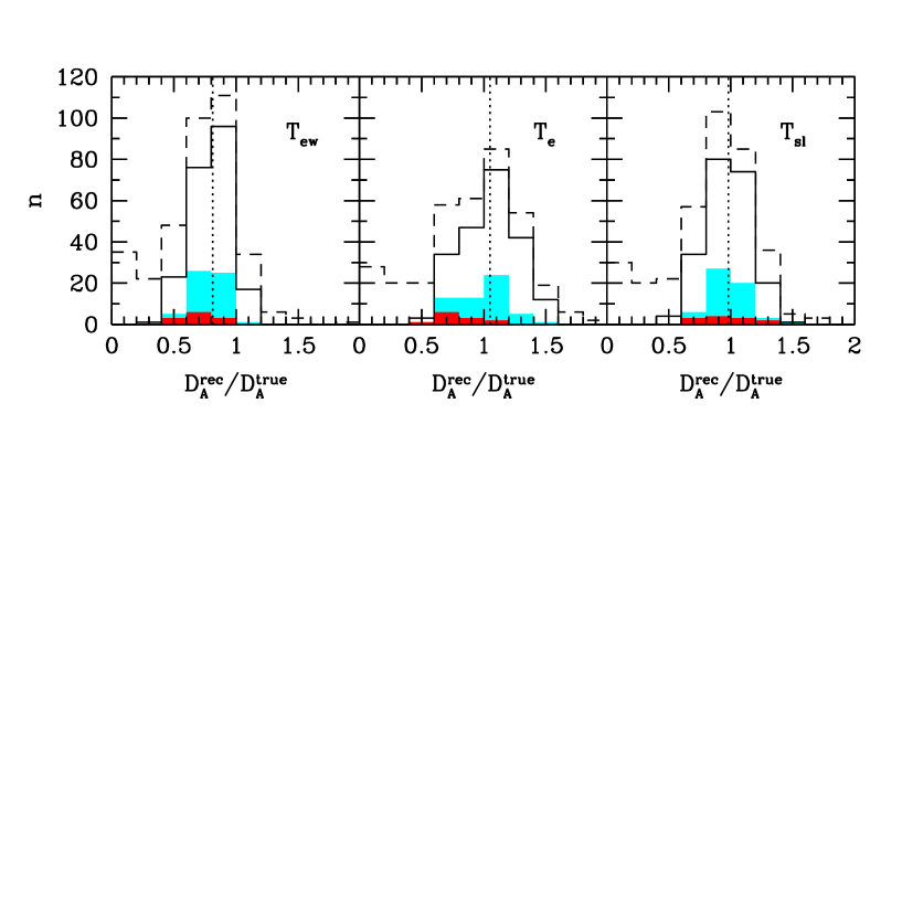
Figure 9: Distributions of the accuracy in recovering the correct value of the angular–diameter distance, $D_{A}^{\rm rec}/D_{A}^{\rm true}$, using the polytropic $\beta$–model for the whole sample (dashed line) and for the subset of regular clusters (solid), using emission–weighted (left panel), electron (central panel) and spectroscopic–like (right panel) temperature. Also shown with the light and dark gray areas are the corresponding distributions for the subset of the clusters with $2.5<T_{sl}(keV)<5$ and $T_{sl}(keV)>5$, respectively. The vertical dotted line in each histogram represents the mean value of the distribution for the sample of regular clusters.

The results obtained for $D_{A}$ are shown in Figure 9, and also reported in Table 1, using emission–weighted, electron and spectroscopic–like temperatures. Quite interestingly, the improved quality of the fit to the profile of the Compton–$y$ parameter now makes the distribution peak at a value much closer to the correct $D_{A}$, independently of whether we use the whole sample or the subsample of relaxed clusters.

The angular–diameter distance is correctly recovered when using either the electron or the spectroscopic–like temperature with deviations which are always $\raise-2.0pt\hbox{\hbox to0.0pt{\hbox{$\sim$}\hss}\raise 5.0pt\hbox{$<$}\ }5$ per cent, on average. This is a rather encouraging result, since it indicates that any bias, induced by using the temperature as measured from X–ray observations, is in fact rather small. Using instead the emission–weighted temperature turns into a systematic underestimate of $D_{A}$ by about 20 per cent, as a consequence of the fact that it is systematically higher than the electron temperature. For all the definitions of temperature we find a significant intrinsic scatter, of about 20 per cent on average, in spite of our selection of regular objects.

The fact that the scatter is stable against the definition of temperature implies that it is almost insensitive to the thermal structure of the ICM and, therefore, to the details of the ICM physics. This scatter instead quantifies the effect of departure from spherical symmetry of the ICM spatial distribution. In fact, the above scatter increases to about 50 per cent, if no preselection of regular clusters is implemented (Table 1). Quite remarkably, the intrinsic scatter calibrated with our simulations is rather close to the 17 per cent value, reported by Hughes & Birkinshaw (1998), for the uncertainty induced by the intrinsic cluster ellipticity.

Similarly to the case of the isothermal fit, we note from Fig. 9 that the low–$D_{A}$ tails of the distributions are contaminated by irregular clusters, for which $D_{A}$ is very badly recovered. For instance, for the irregular cluster shown in Fig. 4 we find $D_{A}^{\rm rec}/D_{A}^{\rm true}=0.30$ when using the electron temperature. Similarly to the case of the isothermal fit, also in this case the distribution of the hot clusters is consistent with that of the regular cluster subset.

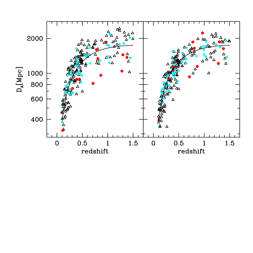
Figure 10: Estimated $D_{A}$ vs. $z$ for the regular cluster sample: 2/3 of this sample was uniformly distributed in the redshift range $0.1<z<0.5$ and 1/3 in the range $0.5<z<1.5$. On the left (right) panel is shown the angular–size distance obtained using the electron (spectroscopic-like) temperature and the polytropic gas model. The symbols indicate clusters spectroscopic temperature: $T_{sl}(keV)<2.5$ (triangles), $2.5<T_{sl}(keV)<5$ (squares) and $T_{sl}(keV)>5$ (circles). The solid line shows the $D_{A}$–$z$ relation for the $\Lambda$CDM cosmology assumed in the simulations.

4.3 Implications for cosmological parameters

The precision in the recovery of the angular–size distance when using the polytropic model indicates that this method is potentially accurate to estimate cosmological parameters. In order to test this we create a simple mock catalog of clusters, which is obtained by distributing 2/3 of our regular clusters uniformly in redshift in the range $0.1<z<0.5$, while the remaining 1/3 is distributed uniformly in the range $0.5<z<1.5$. Recall that each simulated cluster is observed along three orthogonal lines of sight and the redshift of each projection is chosen randomly. Figure 10 shows the resulting distribution of clusters in the $D_{A}$–$z$ plane. We remind here that our simulated clusters have been identified at $z=0$. Therefore, our procedure to distribute them at $z>0$ neglects the effect of their possible morphological evolution. We have been forced to this choice by the small volume of our simulation box, which implies the rapid disappearance of reasonably massive clusters inside the high–redshift simulation box.

For the estimate of the Hubble constant, $H_{0}$, we limit the analysis to the 66 clusters at $z<0.3$. Including high redshift objects would make the recovery of $H_{0}$ progressively more dependent on the knowledge of the underlying cosmology. When using the electron temperature, the distribution of the $H_{0}$ values has mean $H_{0}=70\pm 2\,{\rm km\,s^{-1}Mpc^{-1}}$; when using the spectroscopic temperature this mean is $H_{0}=75\pm 2\,{\rm km\,s^{-1}Mpc^{-1}}$. In both cases the uncertainties are the $1-\sigma$ standard deviations. These values are obtained by assuming the correct cosmology. When assuming the Einstein–de-Sitter model, we find $H_{0}$ biased low by 8 per cent.

As for the estimate of the matter density parameter $\Omega_{m}$, we fix the value of $H_{0}$ to its true value and assume flat geometry. In this case, we use the 73 clusters lying at $z>0.5$. Estimating $\Omega_{m}$ as the average of the values yielded by each cluster would provide unreliable results; in fact, inaccurate values of $D_{A}$ can imply negative values of $\Omega_{m}$, which are clearly unphysical. Therefore, we compute the best–fitting value of $\Omega_{m}$ with a $\chi^{2}$–minimization procedure. To associate the uncertainty to the estimated $\Omega_{m}$, we resort to a bootstrap resampling procedure (e.g. §15.6 of Press et al. 1992). Each bootstrap sample is constructed by randomly selecting, with repetition, the objects from the original sample. Each time that a cluster is selected, its $D_{A}$ is perturbed with a Gaussian random shift with variance 20%, independently of redshift, to account for the “observational” uncertainties. The application of this procedure, when using the electron temperature, gives $\Omega_{m}=0.29\pm 0.05$; we obtain $\Omega_{m}=0.36\pm 0.06$, when using the spectroscopic–like temperature. The uncertainties are the $1-\sigma$ standard deviations computed with 100 bootstrap resamplings. The two temperature definitions provide two $\Omega_{m}$’s whose difference is consistent with the difference in the median values of $D_{A}$. Moreover, and reassuringly, in both cases the central values are consistent with the true value of $\Omega_{m}$.

The small size of the errobars of the estimated $\Omega_{m}$’s should be clearly taken with caution for at least two reasons. First of all, we have assumed errors in $D_{A}$ to be 20 per cent, independently of redshift. High–quality SZ and X–ray observations will eventually allow to bring statistical errors down to this level in the near future. Of course, systematic errors in SZ observations, associated for instance to point–source contamination and CMB signal removal, are different in nature and more difficult to eliminate.

5 Conclusions

In this paper we have applied the method to calibrate the cosmic distance scale from the combination of X–ray and Sunyaev–Zeldovich (SZ) observations to an extended set of hydrodynamical simulations of galaxy clusters. The simulations have been performed with the GADGET2 code, for a flat $\Lambda$CDM model with $\Omega_{m}=0.3$, $h=0.7$ and $\sigma_{8}=0.8$, and include the effect of cooling, star formation and supernova feedback. The aim of our analysis was to understand the possible biases introduced by the assumptions of isothermal gas and the X–ray temperature as a close proxy to the electron temperature, as usually done in the analysis of real clusters. Furthermore, the application of this method to a large set of simulated clusters allows us to quantify the intrinsic scatter associated with a cluster-by-cluster variation of their shapes.

Our main results can be summarized as follows.

(a)

Neglecting the temperature gradients in the application of the $\beta$–model produces a significant underestimate of the central value of the Comptonization parameter, $y_{0}$. In turn, this introduces a severe bias in the estimate of the angular–size distance, $D_{A}$.

(b)

Accounting for the presence of the temperature gradients with a polytropic $\beta$–model substantially reduces this bias to a few per cent level. While this result holds when using either the electron or the spectroscopic–like temperature, using the emission–weighted temperature gives a $\sim 20$ per cent underestimate of $D_{A}$.

(c)

Cluster-by-cluster variations of the asphericity and of the degree of gas clumpiness cause an intrinsic dispersion of about $\sim 20$ per cent in the estimates of $D_{A}$. This dispersion significantly increases in case unrelaxed clusters are included in the analysis.

(d)

The set of simulated clusters is used to generate a mock sample of clusters out to redshift $z=1.5$. By assuming a 20 per cent precision in the estimate of $D_{A}$ for each cluster, we find that the correct value of $H_{0}$ is recovered with a statistical error of $2\,{\rm km\,s^{-1}}$ at 1$\sigma$. Furthermore, assuming a prior for the Hubble constant and flat geometry, we find that also the matter density parameter can be estimated in an unbiased way with a statistical error of $\Delta\Omega_{m}=0.05$.

It is worth reminding here that our results are based on the analysis of simulated X–ray and SZ maps, which are ideal in a number of ways. First of all, they have been generated by projecting the signal contributed by the gas out to about six virial radii. A more rigorous approach would require projecting over the cosmological light cone, to properly account for the fore/background contamination. While projection effects ought to be marginal for the X–ray maps, they may substantially affect the SZ signal (e.g., White et al., 2002; Dolag et al., 2005). Furthermore, our noiseless maps need to be properly convolved with the “response function” of both X–ray and SZ telescopes under realistic observing conditions. Neglecting the observational noise clearly leads to an underestimate of the uncertainties in the determination of the parameters defining gas density and temperature profiles. Accounting for such effects would definitely require passing our ideal maps through suitable tools to simulate X–ray (e.g., Gardini et al., 2004) and SZ observations (e.g., Kneissl et al., 2001; Pierpaoli et al., 2005). Finally, the effect of neglecting the departure from isothermality depends on the physical description of the ICM provided by the simulations. Since simulated clusters have central temperature gradients, which are steeper than the observed ones, the above effect is probably overestimated. This demonstrates that a proper use of hydrodynamical simulations to calibrate galaxy clusters as standard rod also requires a correct description of the physical properties of the intra–cluster gas.

When this paper was ready for submission it came to our attention a paper by Hallman et al. (2005), which reports on an analysis similar to ours. However, their results indicate that assuming an isothermal gas tends to overestimate rather underestimate $D_{A}$, as we find. Clearly, a detailed comparison of their approach with ours would be necessary to understand this discrepancy. We also note that these authors propose a novel method to estimate $D_{A}$ which relies on spatially resolved SZ observations. On the contrary, our suggestion of considering a polytropic gas model can also be applied when the spatial information of the SZ data is poor.

References

- Aghanim et al. (2004) Aghanim N., Hansen S. H., Lagache G., 2004, ArXiv Astrophysics e-prints
- Allen et al. (2001) Allen S. W., Schmidt R. W., Fabian A. C., 2001, MNRAS, 328, L37
- Birkinshaw (1979) Birkinshaw M., 1979, MNRAS, 187, 847
- Birkinshaw (1999) Birkinshaw M., 1999, Phys. Rep., 310, 97
- Birkinshaw & Hughes (1994) Birkinshaw M., Hughes J. P., 1994, ApJ, 420, 33
- Bonamente et al. (2004) Bonamente M., Joy M. K., Carlstrom J. E., Reese E. D., LaRoque S. J., 2004, ApJ, 614, 56
- Borgani et al. (2006) Borgani S., Dolag K., Murante G., Cheng L.-M., Springel V., Diaferio A., Moscardini L., Tormen G., Tornatore L., Tozzi P., 2006, MNRAS, pp 270–+
- Borgani et al. (2004) Borgani S., Murante G., Springel V., Diaferio A., Dolag K., Moscardini L., Tormen G., Tornatore L., Tozzi P., 2004, MNRAS, 348, 1078
- Carlstrom et al. (2002) Carlstrom J. E., Holder G. P., Reese E. D., 2002, ARAA, 40, 643
- Cavaliere et al. (1979) Cavaliere A., Danese L., de Zotti G., 1979, A&A, 75, 322