On stability and spiral patterns in polar disks

To investigate the stability properties of polar disks we performed two-dimensional hydrodynamical simulations for flat polytropic gaseous self-gravitating disks which were perturbed by a central S0-like component. Our disk was constructed to resemble that of the proto-typical galaxy NGC 4650A. This central perturbation induces initially a stationary two-armed tightly-wound leading spiral in the polar disk. For a hot disk (Toomre parameter $Q>1.7$), the structure does not change over the simulation time of 4.5 Gyr. In case of colder disks, the self-gravity of the spiral becomes dominant, it decouples from the central perturbation and grows, until reaching a saturation stage in which an open trailing spiral is formed, rather similar to that observed in NGC 4650A. The timescale for developing non-linear structures is 1-2 Gyr; saturation is reached within 2-3 Gyr. The main parameter controlling the structure formation is the Toomre parameter. The results are surprisingly insensitive to the properties of the central component. If the polar disk is much less massive than that in NGC 4650A, it forms a weaker tightly-wound spiral, similar to that seen in dust absorption in the dust disk of NGC 2787. Our results are derived for a polytropic equation of state, but appear to be generic as the adiabatic exponent is varied between $\gamma=1$ (isothermal) and $\gamma=2$ (very stiff).

1 Introduction

Polar ring galaxies (PRGs) are characterized by an early-type or elliptical central component and a gas-rich ring or disk which is nearly polar with respect to the central galaxy. The spatial orientation and the kinematics of the main components makes them “multi-spin systems” (Rubin rubin94 (1994)) with mutually orthogonal spin vectors. In the polar-ring catalog (Whitmore et al. whitmore90 (1990)) about 100 PRGs or PRG candidates are given. The polar structures can be either narrow rings, or radially-extended disks. Both morphologies are about equally frequent.

A prototype of a PRG with a radially-extended disk is NGC 4650A. It is characterized by a central gas-poor S0 component and an exponential polar disk much larger than the central galaxy. At an adopted distance of 35 Mpc, the central component has a luminosity $L_{I}\approx\mbox{$3\cdot 10^{9}$}\leavevmode\nobreak\ \mbox{L${}_{\sun}$}$, corresponding to a mass of $5\cdot 10^{9}$  M_☉ in stars, while for the polar disk $L_{I}\approx\mbox{$1.2\cdot 10^{9}$}\leavevmode\nobreak\ \mbox{L${}_{\sun}$}$, so the stellar mass $3\cdot 10^{9}$  M_☉ (Gallagher et al. gallagher02 (2002)). The polar disk shows roughly an exponential distribution of stellar light (Iodice et al. iodice02 (2002)). It is gas-rich, with an HI-mass of about $7\cdot 10^{9}$  M_☉ at the adopted distance (Arnaboldi et al. arnaboldi97 (1997)), and about 10% as much mass in molecular form (Watson et al. watson94 (1994)). The HI maps show gas rotating at speed 120km s^-1 out to a radius of 25 kpc, which corresponds to a dynamical mass of $8\cdot 10^{10}$  M_☉. The polar disk is blue, with about 1 M_☉ yr^-1 of ongoing star formation, whereas in the S0 component star formation appears to have ceased $3-5\,$Gyrs ago (Gallagher et al. gallagher02 (2002)).

Arnaboldi et al. pointed out the presence of two open spiral arms in the polar disk, with approximate mirror symmetry about the central S0, in both optical and near-infrared light. These have a spatial extent of about 20 kpc in diameter (see their Fig. 10 or our Fig. 13 below). The arms are also traced by a few blue knots, suggesting that they represent real density enhancements where stars have formed, and not simply a warp in the polar disk (Gallagher et al. gallagher02 (2002)).

The polar disk in NGC 2787, which is classified SB0/a with a LINER nucleus, exhibits a very different morphology, with a tightly-wound spiral in the inner 7 arcsec or 200 pc of the polar disk. The HST/WFPC2 image (see Figure 13 of Erwin & Sparke erwin03 (2003) or Figure 4 of Sil’chenko & Afansiev silchenko04 (2004)) shows the spiral in dust absorption SE of the nucleus where the polar disk lies in front of the galaxy. The central galaxy is about as luminous as NGC 4650A, with $L_{B}\approx\mbox{$2\cdot 10^{9}$}\leavevmode\nobreak\ \mbox{L${}_{\sun}$}$ at a distance of 7.5 Mpc, and probably has a similar mass. But the polar structure is much less massive, with only $3\cdot 10^{8}$  M_☉ of HI and H₂ (Welch & Sage welch03 (2003)), and most of this is in a ring at radius $\sim 6.4$ arcmin or 14 kpc.

Though polar ring galaxies (PRGs) are not very frequent (about 0.5% of all galaxies (Whitmore et al. whitmore90 (1990))), they attracted the interest of astronomers mainly for two reasons. First, the fact that they are multi-spin systems makes them prime targets to study rotation curves in orthogonal directions. From that, the flattening of dark haloes might be deduced (e.g. Whitmore et al. whitmore87 (1987), Sackett & Sparke sackett90 (1990), Sackett et al. sackett94 (1994)). Second, their formation mechanism is still under debate though it is assumed that galaxy interactions play a key rôle. Basically two formation concepts have been discussed in the past. One scenario is a tidal accretion model, in which mass is transferred in an encounter between two galaxies (e.g. Reshetnikov & Sotnikova reshetnikov97 (1997)). The second assumes a head-on merger between two orthogonal spiral galaxies (Bekki bekki98 (1998)). Bournaud & Combes (bournaud03 (2003)) performed numerical simulations to compare the probability of both scenarios, favouring the accretion scenario. However, a lot of assumptions which are observationally hard to determine enter the estimate of the probabilities for both scenarios.

In order to understand the formation and evolution of polar disks, their ages and, thus, their stability properties are of special interest. From their regular morphology, many appear to be stable on at least several dynamical timescales (see e.g. Sparke sparke2004 (2004) for a review). If so, differential precession effects have to be suppressed effectively. Steiman-Cameron & Durisen (steiman82 (1982)) suggested that a non-spherical halo might be a stabilizing factor. Sparke (sparke86 (1986)) and Arnaboldi & Sparke (arnaboldi94 (1994)) emphasized that self-gravity may stabilize polar disks. Especially, in massive polar disks like in NGC 4650A self-gravity is expected to be important.

In this paper, we want to investigate the stability properties of self-gravitating polar disks which are perturbed by a central galactic component. Our numerical analysis is based on two-dimensional simulations for flat disks. Such calculations have been widely used for modelling stellar and gaseous disks (e.g. Englmaier & Shlosman englmaier00 (2000), Orlova et al. orlova02 (2002), Masset & Bureau masset03 (2003)), for simulating star-forming disks (e.g. Korchagin & Theis korchagin99 (1999)) or dusty nuclear disks (Theis & Orlova theis04 (2004)). This numerical approach allows not only to study the evolution during the linear stage, but also to follow the system deeply into the non-linear regime. From that we get e.g. the timescales of the different evolutionary stages or the spatial pattern and kinematics of the system.

The numerical code is described in Sect. 2. In Sect. 3 the initial model is presented. The numerical simulations are given in Sect. 4 and 5. Finally, we discuss and summarize our results in Sect. 6.

2 Hydrodynamic code

2.1 Numerical Method

In our simulations we solve the two-dimensional hydrodynamical equations for a flat disk in cylindrical coordinates (with $z=0$). This represents a polar ring or disk around a galaxy that is flattened in the $x-z$ plane, as shown in Figure 7. In some images cartesian coordinates are shown: then the positive $x$-axis corresponds to $\varphi=0$ and $\varphi$ increases counter-clockwise. We solve the

1. continuity equation for the surface density $\Sigma(R)$

   $$\frac{\partial\Sigma}{\partial t}+\frac{1}{R}\frac{\partial(R\Sigma u)}{\partial R}+\frac{1}{R}\frac{\partial(\Sigma v)}{\partial\varphi}=0$$ (1)

2. the Euler equation for the radial velocity $u$

   $$\frac{\partial u}{\partial t}+u\frac{\partial u}{\partial R}+\frac{v}{R}\frac{\partial u}{\partial\varphi}-\frac{v^{2}}{R}+\frac{1}{\Sigma}\frac{\partial P}{\partial R}+\frac{\partial\Phi}{\partial R}=0$$ (2)

3. the Euler equation for the azimuthal velocity $v$

   $$\frac{\partial v}{\partial t}+u\frac{\partial v}{\partial R}+\frac{v}{R}\frac{\partial v}{\partial\varphi}+\frac{vu}{R}+\frac{1}{\Sigma}\frac{\partial P}{\partial\varphi}+\frac{1}{R}\frac{\partial\Phi}{\partial\varphi}=0$$ (3)

The gravitational potential $\Phi\equiv\Phi_{\rm disk}+\Phi_{\rm hb}+\Phi_{\rm bar}$ consists of three components: the polar disk, a halo/bulge, and a contribution from the flattened S0 galaxy. The gravitational potential $\Phi_{\rm disk}$ of the flat polar disk is given by (Binney & Tremaine binney87 (1987), hereafter BT87, Sect. 2.8)

$$\Phi_{\rm disk}(R,\varphi) = -G\int_{0}^{\infty}R^{\prime}dR^{\prime}\cdot$$ (4)

$$\int_{0}^{2\pi}\frac{\Sigma(R^{\prime},\varphi^{\prime})d\varphi^{\prime}}{\sqrt{{R^{\prime}}^{2}+R^{2}-2RR^{\prime}\cos(\varphi^{\prime}-\varphi)}}\,.$$

This sum is calculated using a FFT technique applying the 2D Fourier convolution theorem for polar coordinates. External potentials describe the contribution of a rigid halo/bulge. The latter can be done in two ways: either a halo/bulge mass distribution is given from which the equilibrium rotation curve is derived (considering also the pressure forces and the self-gravity of the disk) or the rotation curve $v_{c}(R)$ is given and the halo/bulge mass distribution is derived. In the latter case (which we used here), the contribution $\partial\Phi_{\rm hb}/\partial R$, i.e. the enclosed mass of the halo/bulge component, is calculated from

$$v_{c}^{2}(R)=R\frac{\partial}{\partial R}(\Phi+\Phi_{\rm hb})\,.$$ (5)

Though formally, any profile of $\Phi_{\rm hb}$ might be a solution of Eq. (5), we only accept physically meaningful, radially increasing cumulative mass distributions. More details of our setup of the rotation curve can be found in Sect. 3.2.

In the $x-y$ plane of the polar material, the oblate S0 galaxy is represented by the bar-like potential of a stationary Ferrers’ bar (BT87, Sect. 2.3). In order to avoid an initial ”kick” on the disk, the mass $M_{\rm bar}$ of the bar-like perturbation is slowly enhanced starting from $M_{\rm bar}(t=0)=0$. During this adiabatic turn-on process the mass $M_{\rm hb,<a}$ of the halo/bulge inside the semi-major axis $a$ is reduced by keeping the sum of the masses $M_{\rm bar}(t)+M_{\rm hb,<a}(t)={\rm const}$.

For the pressure terms we applied a polytropic equation of state

$$P=C\cdot\Sigma^{\gamma}$$ (6)

with an adiabatic exponent of $\gamma=5/3$. This allows to close the set of hydrodynamical equations with the equations for the first order moments, i.e. the Euler equations (2) and (3). The hydrodynamic equations (1) – (3) are discretized on a logarithmic Eulerian grid with a constant logarithmic grid spacing. The different terms in the equations (1) – (3) are taken into account by applying an operator splitting technique like e.g. in the ZEUS program (Stone & Norman stone92 (1992)). Advection is performed by the second-order van-Leer scheme. The timestep is determined according to the usual Courant-Friedrichs-Levy criterion. For our simulations we use reflecting boundary conditions in radial direction (and periodic in azimuthal direction). Our simulations are mainly done on a grid with 270x270 cells.

Most of the simulations are performed without any explicit artificial viscosity (AV). Test calculations with different amounts of AV did not significantly differ from the reference simulation without AV. During the phase of linear growth the global amplitudes show almost no quantitative difference. Later, in the saturation stage, shocks become more important and AV gives different results. However, the saturation levels just scatter around the models without AV. Because of that and because we are mainly interested in the growth time for an instability, we did not apply AV in most of the simulations, though it might improve the treatment of shocks in the late saturation stage.

2.2 Units

The units are chosen to be $10^{9}\leavevmode\nobreak\ \mbox{M${}_{\sun}$}$ and 1 kpc for the mass and length scale, respectively. The gravitational constant was set to $G=1$. This results in a velocity unit of 65.6 km s^-1 and a unit for the angular speed of 65.6 km s^-1 kpc^-1. The time unit is 14.9 Myr. These units are used throughout the paper, unless other units are given explicitly.

2.3 Dimensions, Times and Accuracy

Motivated by the polar disk of NGC 4650A we adopted an inner edge of 2 kpc for most of our simulations. The outer edge is set to 50 kpc to prevent perturbations generated at the outer edge from affecting the solutions in the “central” area of the polar disk (10 kpc). When using a total of 270 radial grid cells, our logarithmically equidistant grid has a radial cell size of 24 pc at the inner edge degrading to 0.6 kpc at the outer boundary.

A typical simulation run needs of the order of several $10^{4}$ to $10^{5}$ timesteps, until the end of the calculation at $t=300\approx 4.47$ Gyr is reached. A typical timestep is of the order of $\Delta t\sim 1\dots 6\cdot 10^{-3}\sim 1.5\dots 9\cdot 10^{4}$ yr. The simulations were performed on a NEC-SX5 vector computer. The code is highly vectorized, reaching up to 50% of the peak performance of a single vector processor (sustained performance: 1.6-2 GFlop). The most time-consuming part of the simulations is the calculation of the disk’s self-gravity. Numerically this is done with a fast Fourier transform from the MathKaisan library on the NEC-SX5 computer which is especially fast for this number of grid cells. The usual number in that resolution regime is $256=2^{8}$ cells per dimension. However, the speed of the FFT becomes rather slow for this array size due to bank conflicts in the memory access.

For the simulation of the unperturbed disk (model A) the energy was conserved to better than $5\cdot 10^{-8}$ (relative deviation), angular momentum better than $2\cdot 10^{-8}$ and the mass even within the machine accuracy of double-precision numbers. The accuracy of the code decreases when the system becomes non-linear and the saturation regime is reached. In that case the accuracy is of percent level for both, energy and angular momentum.

3 Initial model

In order to mimic real polar disks to a reasonable degree the parameters for our initial model were chosen to match closely the observations of the prototype polar disk NGC4650A (Gallagher et al. gallagher02 (2002)). However, we do not intend to have a near-to-exact model for NGC4650A, but a “prototypical” polar disk. Thus we preferred to describe the rotation curve or the mass distribution by “simple” standard formulas instead of matching exactly small- or intermediate-scale variations. We also do not consider the multi-phase nature of the ISM or (energy feedback from) star formation in our calculations. In detail the model is characterized by the mass distribution, the kinematics of the disk and the applied equation of state.

3.1 Polar disk

In our standard model, a mass of $M_{\rm disk}=1.2\cdot 10^{10}\leavevmode\nobreak\ \mbox{M${}_{\sun}$}$ is distributed exponentially with a scale length of 4 kpc. The “punched” disk has a sharp inner boundary at a radius of 2 kpc. The half-mass radius of the disk is about 7.3 kpc, and 90% of its mass lies within the ’central’ region at $R<16$ kpc. Additionally, the surface density is slightly perturbed resulting in a random deviation from the mean surface density of an amplitude of $10^{-6}$.

3.2 Rotation curve

Figure 1: Rotation curve $v_{c}$ and contributions of the different components ($v_{\mathrm{hb}}$: halo&bulge, $v_{\mathrm{disk}}$: polar disk and $v_{P}$: pressure) for the unperturbed model A. Note that the contributions are added up quadratically for $v_{c}^{2}$.

In principle our code allows us to adopt any prescribed rotation curve by adjusting the halo/bulge mass distribution accordingly. In order to determine the required halo/bulge potentials the gravity of the disk as well as the pressure gradient terms are taken into account. They are subtracted from the rotation curve in order to get the remaining halo contribution. Though this scheme allows always for a formal solution, only physical cases are accepted by requiring that the enclosed halo/bulge mass is monotonically increasing with radius. The halo/bulge potential is non-rotating. The bar-like S0 component is treated as stationary except for a short, merely technical ”adiabatic” start phase (which is described below).

For the models in this paper we parametrized the rotation curve by

$$v_{c}(R)=v_{\infty}\cdot\frac{R/R_{\rm flat}}{\left[1+\left(R/R_{\rm flat}\right)^{n}\right]^{1/n}}\,\,.$$ (7)

This guarantees a rigid rotation in the inner parts and a flat rotation curve outside. The parameter $n$ defines the smoothness of the transition between these two zones. For our simulations we mainly used a sharp transition near $R_{\rm flat}=2$ kpc by choosing $n=10$. Hence, the rotation curve is basically flat all over the polar disk (Fig. 1).

The initial azimuthal velocity of the gaseous phase is calculated by the Jeans’ equation for the radial velocity component which reads in cylindrical coordinates

$$\frac{\partial u}{\partial t}+u\frac{\partial u}{\partial R}+\frac{v}{R}\frac{\partial u}{\partial\phi}-\frac{v^{2}}{R}=-\frac{1}{\Sigma}\cdot\frac{\partial P}{\partial R}-\frac{\partial}{\partial R}\left(\Phi+\Phi_{\rm hb}\right)\,\,.$$ (8)

In case of the initial equilibrium, the radial velocity $u$ vanishes. If we define the pressure contribution $v_{P}$ to the rotation curve as

$$v_{P}^{2}\equiv-\frac{R}{\Sigma}\cdot\frac{\partial P}{\partial R}\,\,,$$ (9)

then the azimuthal velocity $v$ is given by

$$v^{2}=R\frac{\partial}{\partial R}\left(\Phi+\Phi_{\rm hb}\right)+\frac{R}{\Sigma}\cdot\frac{\partial P}{\partial R}=v_{c}^{2}(R)-v_{P}^{2}(R)\,\,.$$ (10)

The rotation curve is derived from the gravitational potential according to Eq. (5).

Decomposing disk and halo contributions, we find that our disk is submaximal by a factor of 3.6. This leaves sufficient mass for an additional central component. It should be noted that close to the inner edge the gravitational pull of the disk becomes negative, i.e. points outwards. This ”repulsive” force has to be compensated for by a halo contribution corresponding to a rotational velocity exceeding the rotation curve.

We choose the rotation speed $v_{\infty}$ at large radii to be 150 km s^-1. The rotation period at the inner edge is 5.9 time units ($\approx$ 90 Myr) increasing to $\sim$ 300 Myr at the half-mass radius of the disk and reaching $\sim$ 2 Gyr at its outer edge at 50 kpc. The maximum of $\Omega(R)-\kappa(R)/2$ is important for the existence of inner Lindblad resonances: here $\kappa$ is the epicyclic frequency and $\Omega=v_{c}/R$ the circular speed. This maximum is reached at 2.55 kpc where $\Omega-\kappa/2=0.236$ or $=15.4$ km s^-1 kpc^-1. In case of pure stellar disks, a two-armed spiral pattern rotating at the angular rate $\Omega_{p}$ can propagate only where $|\Omega_{p}-\Omega|<\kappa/2$, so any such spiral with $\Omega_{p}<0.236$ cannot propagate from the outer disk to the inner boundary. In our study we deal, however, with gaseous disks, in which density waves can propagate as sound waves through the Lindblad resonances, with little damping (for a brief summary see Bertin (bertin00 (2000)), hereafter GB00, Chap. 16). Polar rings are extremely gas-rich; often more of their baryonic mass is in cool gas than in stars (e.g. Sparke sparke2004 (2004)). So this is likely to be an appropriate approximation.

3.3 Toomre parameter

Figure 2: Initial radial profile of the Toomre parameter $Q$ for the unperturbed model A and the reference model B. The minimum $Q$ of 1.4 is reached at about 6 kpc.

The local stability of a disk with respect to axisymmetric perturbations is controlled by the Toomre parameter

$$Q\equiv\frac{\sigma_{R}\kappa}{\pi G\Sigma}\,\,.$$ (11)

$Q$ compares the stabilizing factors – velocity dispersion $\sigma_{R}$ (sound speed) and radial oscillation frequency (or epicyclic frequency $\kappa$) – with the destabilizing rôle of the self-gravity of a mass element with surface density $\Sigma$ (e.g. BT87 Sect. 6.2). A value of $Q$ less than unity means instability to axisymmetric perturbations. In gaseous disks the most unstable wavelength $\lambda_{m}$ in the radial direction is given by

$$\lambda_{m}\equiv\lambda_{\rm crit}/2$$ (12)

with the critical wavelength $\lambda_{\rm crit}$ defined as

$$\lambda_{\rm crit}\equiv\frac{4\pi^{2}G\Sigma}{\kappa^{2}}\,\,.$$ (13)

From numerical experiments it is known that disks become rather stable even to non-axisymmetric modes for minimum $Q$-values above 1.4. In case of flat rotation curves one can derive from linear stability analysis that $Q>\sqrt{3}\approx 1.73$ guarantees that a fluid disk is stable with respect to all perturbation modes (see e.g. Bertin et al. (bertin89 (1989)), Polyachenko et al. (polyachenko97 (1997)) or Section 15.2 of GB00). This is also in good agreement with multi-component disks studied by Orlova et al. (orlova02 (2002)). In our reference model the constant $C$ of Eq. (6) is adjusted in such a way that the initial minimum value of $Q$ is 1.4. This value is reached at $R\approx 6$ kpc. Fig. 2 shows the radial run of $Q$ for this model.

Table 1: Properties of the numerical models

model	$M_{\rm bar}(\leavevmode\nobreak\ \mbox{M${}_{\sun}$})$	$Q_{\rm min}$	comment
A	–	1.4	no central component
B	$5\cdot 10^{9}$	1.4	reference model
			(with central component)
MB1	$1\cdot 10^{9}$	1.4	small S0 component
MB2	$1\cdot 10^{10}$	1.4	”maximum” S0 component
MB3	$5\cdot 10^{9}$	1.4	$n_{b}=-1$ non-homogeneous S0 comp.
MB4	$5\cdot 10^{9}$	1.4	$n_{b}=-2$, ”isothermal” S0 comp.
T1	$5\cdot 10^{9}$	1.4	$t_{\rm adi}=100$, long switch-on
T2	$5\cdot 10^{9}$	1.4	temporary S0 comp. (off at $t=100$)
Q1	$5\cdot 10^{9}$	1.3	varied Toomre parameter
Q2	$5\cdot 10^{9}$	1.5
Q3	$5\cdot 10^{9}$	1.6
Q4	$5\cdot 10^{9}$	1.7
Q5	$5\cdot 10^{9}$	1.8
Q6	$5\cdot 10^{9}$	1.9
			varied mass of the polar disk
MD1	$5\cdot 10^{9}$	1.4	$6.0\cdot 10^{9}$   M☉
MD2	$5\cdot 10^{9}$	1.4	$6.0\cdot 10^{9}$   M☉, but $Q_{\rm min}=1.2$
MD3	$5\cdot 10^{9}$	1.4	$2.4\cdot 10^{10}$   M☉
MD4	$5\cdot 10^{9}$	1.4	$3.7\cdot 10^{10}$   M☉, maximum disk
R1	$5\cdot 10^{9}$	1.4	varied rotation profile, n=6
R2	$5\cdot 10^{9}$	1.4	n=3
S1	$5\cdot 10^{9}$	1.4	varied Eq. of state, $\gamma=2.0$
S2	$5\cdot 10^{9}$	1.4	$\gamma=1.0$ (isothermal)
S3	$5\cdot 10^{9}$	2.1	$\gamma=1.0$ (isothermal), $Q_{\rm min}=2.1$
G1	$5\cdot 10^{9}$	1.4	larger grid (686x686)
G2	$5\cdot 10^{9}$	1.4	inner edge at $R_{\mathrm{min}}=1$ kpc
G3	$5\cdot 10^{9}$	1.4	as G2, but smooth transition of $\Sigma$
G4	$5\cdot 10^{9}$	1.2	as G3, but reduced $Q_{\mathrm{min}}$

4 Models without an S0-like central component

The aim of this paper is to study the stability of polar disks perturbed by a central S0-like component. As a test of the code, but also for comparison with the models of the following sections, we first describe in Sect. 4 the evolution of an unperturbed gaseous disk (model A). In Sect. 5 we perturb the polar disk by a central S0-like component. A list of the models described in this paper is given in Table 1.

Figure 3: Perturbation of the surface density profile at the end of the simulation of model A ($t=300$). Contour lines are given in $\leavevmode\nobreak\ \mbox{M${}_{\sun}$}\,{\rm pc}^{-2}$ starting from 0.1 to 0.9 $\leavevmode\nobreak\ \mbox{M${}_{\sun}$}\,{\rm pc}^{-2}$ with a difference of 0.2 $\leavevmode\nobreak\ \mbox{M${}_{\sun}$}\,{\rm pc}^{-2}$ between the contour lines. For comparison, the unperturbed surface density at a distance of 5 kpc is 37.2 $\leavevmode\nobreak\ \mbox{M${}_{\sun}$}\,{\rm pc}^{-2}$.

In the first set of simulations, we investigate the evolution of an isolated galactic disk which has a central hole as described in the previous section. Such a disk is characterized by an exponential mass profile, a basically flat rotation curve and a Toomre parameter of $Q=1.4$, a value slightly above the one required for stability against axisymmetric perturbations.

Inspecting the Lagrange radii, i.e. radii containing a constant mass fraction, we see that the system is radially stable: the relative changes of the Lagrange radii are less than 0.01% over the whole integration time of $t=300=4.47$ Gyr. On the other hand, the surface density profile shows the development of a pronounced two-armed trailing spiral structure until the end of the simulation (Fig. 3). The spirals are tightly wound in agreement with a short critical wavelength $\lambda_{\rm crit}$ of about 3 to 4 kpc. The most unstable wavelength is then about $\lambda_{m}\sim 1.5-2\,\,{\rm kpc}$ for a gaseous disk (BT87) which reproduces roughly the wavelengths visible in Fig. 3. The maximum amplitudes of the perturbed density $\Delta\Sigma(R,\varphi,t)\equiv\Sigma(R,\varphi,t)-\Sigma(R,\varphi,t=0)$ are below 1 $\leavevmode\nobreak\ \mbox{M${}_{\sun}$}\,{\rm pc}^{-2}$. Normalized to the initial densities, $\Delta\Sigma/\Sigma$ is much less than 1%, which would not be detectable in observations of real galaxies.

Another way to visualize the nature and growth of instabilities in disks is to consider the azimuthal Fourier modes $a_{m}$ at different radii. They are calculated for $m\neq 0$ by (cf. also Laughlin et al. laughlin98 (1998))

$$a_{m}(R,t)\equiv\frac{1}{2\pi}\int_{0}^{2\pi}\Sigma(R,\varphi,t)e^{im\varphi}d\varphi\,\,.$$ (14)

Their phase angle is then given by

$$\phi_{m}(R,t)\equiv\tan^{-1}\left\{\frac{\Im[a_{m}(R,t)]}{\Re[a_{m}(R,t)]}\right\}$$ (15)

This phase angle is a measure for the spatial orientation of the related perturbation. E.g. a bar described by $\Sigma(R,\varphi)=\Sigma_{0}(R)\cdot\{1+A\cos[2(\varphi-\alpha)]\}$ has its major axis along $\varphi=\alpha$ or $\varphi=\alpha+\pi$, respectively. The corresponding phase angle for the $m$-mode is $\phi_{m}(R)=m\alpha$. Thus, the pattern speed for a mode $m$ can be calculated by

$$\Omega_{p}(R,t)\equiv\frac{1}{m}\frac{d\phi_{m}(R,t)}{dt}\,\,.$$ (16)

A measure for the global structure of a disk are the (radially integrated) global Fourier modes defined by

$$C_{m}(t)\equiv\frac{2\pi}{M_{\rm disk}}\int_{R_{\rm low}}^{R_{\rm hig}}a_{m}(R,t)RdR\,\,.$$ (17)

$M_{\rm disk}$ is the mass of the disk within the radial range $[R_{\rm low},R_{\rm hig}]$. The global Fourier amplitude is the modulus of $C_{m}$, whereas the global growth rate is given by the time derivative of the logarithmic Fourier amplitude, i.e.

$$\gamma_{m}\equiv\frac{d(\ln|C_{m}(t)|)}{dt}\,\,.$$ (18)

It is also common to define a $m=0$-mode which denotes the temporal evolution of the radial mass redistribution:

$$C_{0}\equiv\frac{2\pi}{M_{\rm disk}}\int_{R_{\rm low}}^{R_{\rm hig}}|\bar{\Sigma}(R,t)-\bar{\Sigma}_{0}(R)|RdR\,\,.$$ (19)

We adopted $R_{\rm low}=2$ kpc and $R_{\rm hig}=50$ kpc, integrating over the entire disk. $\bar{\Sigma}(R,t)$ and $\bar{\Sigma}_{0}(R)$ are the azimuthally averaged surface densities at time $t$, or at the start of the simulations, respectively. As long as the evolution is well described by a linear approach, no radial mass transport should occur. Thus, the increase of $C_{0}$ is a good indicator for the onset of non-linear effects.

Figure 4: Temporal evolution of the global Fourier modes for $m=1,\dots,4$ of model A. The mode $m=0$ describes the radial matter redistribution. For details see text.

Fig. 4 shows the temporal evolution of the global Fourier modes for the ”punched” disk without a central component. Starting from a low noise level, the even modes $m=2,4$ are the dominant ones describing a basically two-armed structure. In agreement with predictions of linear stability analysis they grow exponentially on a similar, but long timescale of $\gamma_{m}^{-1}\sim 20\approx 300$ Myr. In a late stage the $m=3$-mode grows, too, whereas the $m=1$-mode remains stable throughout the whole simulation. Until the end of the simulation the system never reaches the regime of non-linear growth or saturation. The amplitudes reached after 4.4 Gyr are so low that in real galaxies they would be practically invisible.

The $C_{0}$-amplitude shows a small initial radial mass redistribution which is caused by the small deviations from equilibrium due to the imprinted initial density perturbation. After quickly establishing a new equilibrium, the system remains radially stable.

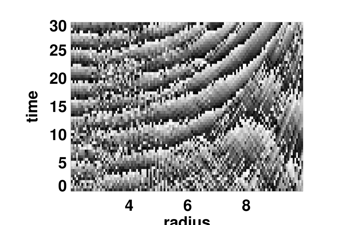
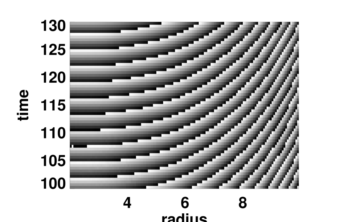
Figure 5: Evolution of the phase angle $\phi_{m}$ of model A for the $m=2$ mode during the initial stage (upper diagram) and the growing stage (lower diagram) (0^∘: white; 360^∘: black).

The evolution of the phase angles gives more detailed information on the structure formation. During the initial stage of the simulation no large scale pattern is discernible. However, after time $t\sim 10$ coherent features are detectable for the phase angle of the $m=2$ mode which become more and more prominent indicating the weak two-armed structure of the system (Fig. 5, upper diagram). The structure grows from inside out, starting at a distance of about 4 kpc, well outside the inner edge of the computational grid. Therefore, it is very unlikely that the growing instability is caused by the sharp cut-off due to the central hole of the disk or by boundary effects.

Figure 6: Evolution of the radially averaged ($R<10\mathrm{kpc}$) pattern speed of the $m=2$ mode (solid) and its mean deviation (dashed, lower curve) for model A.

In a later stage when the linear growth is well established the tightly wound spiral structure is clearly visible in the phase angles (Fig. 5, lower diagram). These allow an accurate determination of the intrinsic pattern speed of the two-armed spiral in the late stage as $\Omega_{p,m=2}\approx 1.07\approx 70$ km s^-1kpc^-1 (Fig. 6). $\Omega_{p,m=2}$ is the radial average of the local pattern speed $\Omega_{p}(R,t)$ within the innermost 10 kpc. The small mean deviations of $\Omega_{p}(R,t)$ within this region indicate also the formation of a large-scale $m=2$ pattern after $t=50$. For this pattern speed, there are no inner Lindblad resonances and corotation is close to but inside the inner boundary of the grid. Similar to the $m$=2 mode, regular patterns are also found for the $m$=3- and $m$=4-modes. Their pattern speeds are slightly smaller than that of the $m$=2 mode (by 4% and 7%, respectively). However, they are still too large to yield corresponding ILRs.

5 Models with a central perturbation

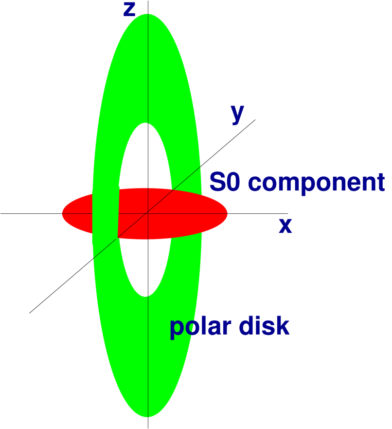
Figure 7: Schematic view of the geometry of the simulated polar disk.

In this section we describe the evolution of ”punched” disks perturbed by a central S0- or elliptical-like component as a model for polar disks.

The perturbation due to the S0 galaxy is given by the stationary potential of a Ferrers’ bar which has a density distribution (BT87, Sect. 2.3)

$$\rho_{b}(m^{2})=\rho_{0}\cdot\left(1-m^{2}\right)^{\displaystyle n_{b}}\cdot\Theta(1-m)\,\,.$$ (20)

$\Theta$ is here the Heaviside function and $m^{2}=(x/a)^{2}+(y/b)^{2}+(z/c)^{2}$ a modified radial coordinate. For most of our simulations we choose $n_{b}=0$ assuming a homogeneous mass distribution. In our reference model, the total mass of the central component is set to $M_{\rm bar}=5\cdot 10^{9}\,\,\leavevmode\nobreak\ \mbox{M${}_{\sun}$}$.

The S0 galaxy’s major axis has a radial extent of 1 kpc, so the S0 disk lies completely inside the central hole of the polar disk. The axis ratios are set to $b/a=1$ and $c/a=0.4$ corresponding to an oblate spheroid. The minor axis points to the $z$-axis of the coordinate system. Thus, the ”disk” of the central component is located in the $x$-$y$-plane and the polar disk is in the $y$-$z$-plane. Hence, the disk plane of the central component corresponds to the abscissa of the polar disk snapshots, while the axis of the ordinate points to the $z$-axis, perpendicular to the disk plane of the central S0 component (as shown in Fig. 7).

In order to avoid switch-on effects, the bar-like potential of the central S0 component is turned on slowly on a timescale of $t_{\rm adi}=20\approx 300$ Myr. During that time the mass of the S0 component is increased, while the same amount of mass is subtracted from the bulge/halo contribution.

5.1 The reference model

Figure 8: Rotation curve $v_{c}$ of a polar disk including a central component (model B). Shown are the contributions of the different components ($v_{\mathrm{halo}}$: halo, $v_{\mathrm{disk}}$: disk, $v_{P}$: pressure and $v_{\mathrm{S0}}$: S0 component).

In order to start with a model resembling closely model A without a central component, we kept the rotation curve and the mass distribution in the polar disk constant, but added the central perturbation with $M_{\rm bar}=5\cdot 10^{9}\,\,\leavevmode\nobreak\ \mbox{M${}_{\sun}$}$ (model B). Due to the additional gravitational force generated by the central component, less mass is now in the halo. However, the velocity curve is still halo-dominated (Fig. 8).

Figure 9: Temporal evolution of the global modes of model B for $m=1,\dots,4$. The mode $m=0$ describes the radial matter redistribution.

Figure 10: Temporal evolution of the Lagrange-radii containing 0.1%, 1%, 5%, 10% (thick line), 20%, 50% (dashed), 75%, 90% (thick) and 99% of the disk mass for model B.

Figure 11: Perturbation of the surface density profile of model B during the linear regime ($t=60=890$ Myr). Contour lines are given in   M_☉ pc^-2 starting from 0.1 to 0.9   M_☉ $\mathrm{pc}^{-2}$ with a difference of 0.2   M_☉ $\mathrm{pc}^{-2}$ between the contour lines. The surface density at 10 kpc is about $10\leavevmode\nobreak\ \mbox{M${}_{\sun}$}$ $\mathrm{pc}^{-2}$. Note the leading arms of the formed pattern.

Figure 12: Surface density profile in the saturation stage at the end of the simulation of model B ($t=300=4.47$ Gyr). Contour lines are given in   M_☉ pc^-2 starting from 10 to 100   M_☉ $\mathrm{pc}^{-2}$ with a difference of 10   M_☉ $\mathrm{pc}^{-2}$ between the contour lines. The maximum relative density perturbation $\Delta\Sigma/\Sigma_{0}$ is about 5.5 in the knot at (0,-6)and 11.6 near the center.

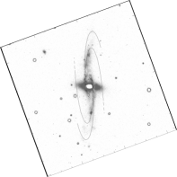
Figure 13: Left, B-band image of NGC 4650A with spiral structure indicated (Figure 10 of Arnaboldi et al. arnaboldi97 (1997)); right, the surface density distribution of Fig. 12 seen in projection, as if the disk is tilted about the y-axis.

The temporal evolution of the global modes (Fig. 9) differs significantly from the simulation without a central perturbation. The perturbed disk develops quickly linearily growing even modes ($m=2$ and $m=4$), whereas the odd modes remain on their initial low level. After a time $t\sim 120\approx 1.8\,\,{\rm Gyr}$ these modes become non-linear, which is reflected in an enhanced growth of the $m=0$-mode. This radial mass redistribution is also shown by the Lagrange radii (Fig. 10). The mass inside the 10%-radius flows inwards, whereas the matter up to the half-mass radius expands. At the time $t\sim 150\approx 2.2$ Gyr the $m=2$-mode reaches its (first) saturation level of about 10%, while the $m=4$-mode reaches a lower amplitude of $\sim 10^{-3}-10^{-2}$. At about the same time the odd modes begin to grow, but they are still linear at the end of the simulation at $t=300$. Therefore, throughout the whole evolution the pattern looks mainly two-armed with a slight modulation introduced by the $m=4$-mode (Figs. 11 and 12).

It is remarkable, however, that the initial spiral pattern is leading (as Fig. 11 shows) whereas the final spiral pattern is trailing like in the unperturbed model A. Moreover, the occurence of an initial leading pattern is found in all our models with a central S0 component. It is especially independent from boundary conditions or other ”technical” parameters.

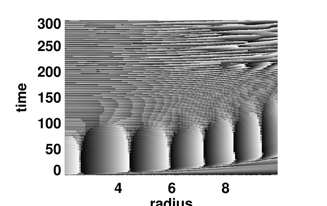
Figure 14: Evolution of the phase angles for the $m=2$ mode (0^∘: white; 360^∘: black).

Figure 15: Evolution of the logarithm of the surface density (in   M_☉ pc^-2) at different times ($t=0$ (upper left), $60$ (upper right), $120$, $180$, $240$, $300$ (lower right)) for model B. For a better visualization of the ”punched” central area a cylinder with a constant level of 3.0 is drawn.

The temporal evolution of the surface density is depicted in Fig. 15: during the linear stage (until $t=120$) a regular tight leading spiral pattern emerges which becomes more and more pronounced. Later, large density variations show up which make the appearance temporarily ring-like. E.g. at $t=180$ there is an almost closed ring at a radius of about 4 kpc. Towards the end of the simulation a new quasi-equilibrium is established. This new mass distribution leads to more open trailing spiral arms in the saturation phase (cf. also Fig. 12). When projected as if seen close to edge-on, the spiral qualitatively resembles that seen in NGC 4650A (Fig. 13). We will show below that this open spiral is essentially independent of the central S0 galaxy, which acts only as a ‘seed’ for its formation. Obviously, the two-armed perturbation created by the central bar-like S0 component induces a mainly two-armed structure in the disk. This becomes clear in the diagram of the phase angles (Fig. 14). Immediately after the start of the simulation a regular, but stationary pattern is formed from inward out. This stationarity can be understood as the response of the flow to the stationary central perturbation. At a time $t\sim 90-100$ this large-scale tight leading pattern vanishes and a rapidly rotating open trailing spiral is formed. The pattern speed (derived from the temporal change of the phase angles) at that time is about $0.9\approx 60$ km s^-1 kpc^-1 which is close to, but lower than the intrinsic pattern speed of the unperturbed disk. The transition from stationary pattern to rotating pattern occurs when the azimuthal force of the growing spiral structure begins to exceed the azimuthal force of the central component. They become comparable for the first time at about $t\sim 85$. Afterwards the azimuthal force of the spirals quickly outnumbers the contribution of the bar-like central component, making the central perturbation unimportant for the further growth of the spiral structure.

5.2 Variation of the central component

In order to test the influence of the central component we varied the mass of the central component (models MB1 and MB2), its switch-on characteristics (model T1) as well as the duration of the central perturbation (model T2).

Figure 16: Temporal evolution of the amplitudes of the $m=0,2$-modes for the reference model B and a small central component ($10^{9}\leavevmode\nobreak\ \mbox{M${}_{\sun}$}$, model MB1).

Figure 17: Temporal evolution of the amplitudes of the $m=0,2$-modes for the reference model B and a maximum central component ($10^{10}\leavevmode\nobreak\ \mbox{M${}_{\sun}$}$, model MB2).

Figure 18: Temporal evolution of the amplitudes of the $m=0,2$-modes for the reference model B and a central component growing slower by a factor of 5 (model T1).

Mass of central component. Simulations with a bar-like S0 component that is five times less massive ($1\cdot 10^{9}\,\,\leavevmode\nobreak\ \mbox{M${}_{\sun}$}$: model MB1) and with a ”maximum S0 component” of $10^{10}\,\,\leavevmode\nobreak\ \mbox{M${}_{\sun}$}$ (model MB2) have been performed. The smaller mass leads to a delayed growth of the spiral modes of the disk by about $t\sim 25\approx 370$ Myr (Fig. 16). In case of the more massive central pertubation there is again a small temporal shift in the behaviour of the amplitudes during the linear stage (Fig. 17). The amplitudes run now ahead by about 100-150 Myr. In both cases the growth rates and the final saturation levels are unaffected by the varied mass of the central component.

We also varied the density profile of the central component by choosing $n_{b}=-1$ (MB3) and $n_{b}=-2$ (MB4). However, even the steeper profile did not change the numerical results significantly.

Timescale of perturbation due to central component. Another test of the influence of the central component is provided by a different temporal behaviour of the perturbing bar-like potential. In model T1 the switch-on time $t_{\rm adi}$ was increased by a factor of 5 to $t_{\rm adi}=100$. Similar to the model MB1 with a less massive central perturbation the growth of the main amplitudes is now delayed by about 400 Myr (Fig. 18). The growth rates and the saturation levels, however, remain unaffected.

Figure 19: Temporal evolution of the amplitudes of the $m=0,2$-modes for the reference model B and model T2 in which the central component is switched off between $t=80$ and $t=100$ (1.2-1.5 Gyr).

Just as in the previous models, even a complete removal of the S0 component does not alter the evolution strongly. Fig.19 shows that the disk quickly evolves on its standard evolutionary path ending up in the same saturation stage, even if the S0 component is switched off before the density perturbations in the disk reach the non-linear regime. The perturbation induced by the S0 component does not disappear when the asphericity of the central perturbation is switched off, and the modes continue to grow. When the gaseous component is dynamically substantially hotter, we find that the excited modes are erased after the perturbation is switched off.

From these calculations we conclude that the modal growth in the reference model B decouples from the initial central perturbation after time $t\sim 100$. The central component acts as a seed for the growing modes, but once these modes are excited, they decouple from the seed growing on a timescale of 1-2 Gyrs. Also other perturbations, e.g. due to gas accretion, might act as such a seed.

5.3 Mass of the polar disk

Figure 20: Temporal evolution of the amplitudes of the $m=2$-modes for the reference model B ($1.2\cdot 10^{10}\leavevmode\nobreak\ \mbox{M${}_{\sun}$}$, plus) and models with different disk masses: MD2 ($6.0\cdot 10^{9}\leavevmode\nobreak\ \mbox{M${}_{\sun}$}$, triangle) and MD3 ($2.4\cdot 10^{10}\leavevmode\nobreak\ \mbox{M${}_{\sun}$}$, filled circle).

The influence of the mass of the polar disk is studied by a small series of simulations starting from half of the mass of the reference model (MD1, MD2) up to the maximum polar disk mass of $3.7\cdot 10^{10}$  M_☉ (MD4). A disk with half the mass of the reference polar disk (or about 1/6 of the maximum polar disk) is very stable (MD1): after an initial adjustment the amplitudes of all modes remain almost constant on a very low level. The dominant $m=2$ and $m=4$ modes are still deep in the linear regime. Only a weak and very tightly wound leading spiral is formed similar to that found in the early stage of the reference model. Model MD2 has the same lowered disk mass as model MD1, but a reduced minimum Toomre parameter $Q_{\rm min}=1.2$. Still the disk is rather stable (Fig. 20) and the dominant even modes have the same amplitude as in MD1. The main difference to MD1 is that the odd modes rise very slowly, but after 4.5 Gyr their amplitudes are still well below those of the even modes.

Increasing the disk mass to twice the mass of the reference model, destabilizes the polar disk (MD3, Fig. 20). The growth rates of the $m=2$ and $m=4$ modes are doubled compared to the reference model. The growth rates of the $m=1$ and $m=3$ modes are very similar to those of the even modes. The overall appearance within the first 2 Gyr, however, is dominated by the even modes because their early amplitude is raised by the perturbation due to the central S0 component. Increasing the mass up to the maximum polar disk (MD4) gives a result very similar to the model with doubled mass MD3.

5.4 The Toomre parameter and the rotation curve

Figure 21: Temporal evolution of the amplitudes of the $m=2$-modes for the reference model B and models Q1 …Q6 with different initial minimum Toomre parameters (Q=1.3,1.6,…,1.9).

An important parameter for the stability of disks is the Toomre parameter. In a series of models we varied the initial minimum $Q$-value between 1.3 and 1.9. Our reference model B was characterized by $Q_{\rm min}=1.4$. Fig. 21 demonstrates the strong dependence of the growth rate on $Q$ during the linear stage: hotter disks are more stable. Close to the reference model (e.g. comparing models with $Q=1.3$ and $Q=1.5$) the growth rate varies less strongly than in models with larger $Q$-values (e.g. the range $Q=1.5$ to $Q=1.7$). Moreover, the disks show a transition to complete stability when the Toomre parameter exceeds a value between 1.7 and 1.8. This is in good agreement with analytical predictions for the transition to stability to be at $Q_{c}\approx 1.73$ (in case of flat rotation curves, see e.g. GB00). The saturation levels of the dominant $m=2$-modes are – in case of unstable configurations – rather similar, i.e. of the order of about 10%.

In the models R1 and R2 we tested the influence of a broader transition region between the rigid rotation domain and the flat part of the rotation curve by setting $n=6$ (R1) and $n=3$ (R2). Model R1 develops qualitatively similar to the reference model B. However, the growth rates of the modes are 30% lower and, therefore, the non-linear regime is first reached after about 3.5 Gyr. In model R2 the transition region is even broader. Still a growing instability is found, but it grows on a longer timescale. The structures dominated by the lower even modes become non-linear at about $t\approx 300\approx 4.5\,\mathrm{Gyr}$. Following the linear stability analysis of Polyachenko et al. (polyachenko97 (1997)) the critical Toomre parameter $Q_{c}$ (for which the system is stable against all perturbations; see their Eq. (36)) drops from $Q_{c}=\sqrt{3}\approx 1.73$ for flat rotation curves to $Q_{c}=\sqrt{3/2}\approx 1.22$ for the rigid rotation region. Thus, a broader transition region results in a reduced $Q_{c}$ beyond the transition radius $R_{\mathrm{flat}}$ compared to the reference model, and the system is expected to be more stable, in agreement with our simulations.

5.5 Equation of state

Figure 22: Temporal evolution of the $m$=2-amplitude for different equations of state: $\gamma$=5/3 (reference model B, plus sign), $\gamma$=2 (model S1, open box) and $\gamma$=1 with $Q_{\mathrm{min}}$=1.4 (model S2, open triangle) and $Q_{\mathrm{min}}$=2.1 (model S3, filled circle).

In the models S1 to S3 we changed the equation of state by varying the adiabatic exponent $\gamma$ in the polytropic equation of state. In model S1 $\gamma$ was set to 2 which is often adopted to mimic stellar disks (e.g. Orlova et al. orlova02 (2002)). Still such a disk is not stable, however the growth of the Fourier amplitudes is delayed and smaller (Fig. 22). Such a stabilizing behaviour can be understood from the stiffer equation of state for $\gamma=2$ which hinders perturbations from growing.

Correspondingly, the disk is expected to be more unstable when the equation of state is less stiff as e.g. in the isothermal case $\gamma=1$. Here cooling is taken to be so efficient that all the heat of compression is dissipated immediately, so that the disk is maintained in an isothermal state, as suggested by Lodato & Rice (2005). Accordingly, we see that model S2 reaches the non-linear regime in about half the time of the reference model. However, the destabilizing effect of the reduced stiffness can be partly compensated for by an initially hotter disk, as model S3 with a minimum Toomre parameter of $Q_{\mathrm{min}}=2.1$ demonstrates. The cases $\gamma=1,5/3$ and 2 are expected to bracket the expected cooling behaviour in real disks.

5.6 Miscellaneous

Figure 23: Temporal evolution of the amplitudes of the $m=0,2$-modes for the reference model B (270x270) and a model G1 with increased grid size (686x686).

We tested different variations of ”technical” parameters which did not result in substantial quantitative deviations from the reference models. E.g. we varied the numerical timestep criterion, we compared with models using different amounts of artificial viscosity or we changed the grid size. As an example Fig. 23 demonstrates the insensitivity of the numerical results on the grid size. Though the resolution was more than doubled, the amplitudes characterizing the dominant mode or the radial mass redistribution evolve qualitatively in the same way and quantitatively almost identical.

In order to test the influence of the inner boundary we rerun the unperturbed model A, but with an inner edge at $R_{\mathrm{min}}=1\mathrm{kpc}$ (models G2 and G3). In both models we kept the total disk mass constant. In model G2 the exponential disk was extended down to a radius of 1 kpc, while in model G3 the surface density was exactly exponential outside a radius of 2 kpc (like in model A), but had a smooth transition to zero from a radius of 2 kpc down to the inner edge. Both models were more stable than model A. In model G2 the growth rate of the dominant $m=1$-mode is a factor two smaller than the growth rate of the dominant mode $m=2$ in model A. Model G3 shows no significant growth at all. In model G4 the same smooth surface density distribution as in model G3 was used, but the minimum Toomre parameter was reduced to 1.2. In that case, the model becomes violently unstable after 4 Gyr. This means that the stabilizing effect of a smoother mass distribution can be compensated by a slightly reduced minimum Toomre parameter. Taking into account that the velocity dispersions within the polar disk are poorly known (if at all), the uncertainties related to the mass distribution at the inner edge of the disk are less critical, unless the profile of the Toomre parameter can be constrained in more detail.

6 Discussion and summary

We investigated the stability properties of polar disks by 2-dimensional hydrodynamical simulations of flat disks perturbed by a non-rotating bar-like potential mimicking a central S0-like component. The properties of the polar disk and the central perturbation were derived from observations of the prototypical polar ring galaxy NGC4650A. We modelled the polar ring by a disk with a “punched” central hole and an exponential mass distribution embedded in a halo with a mainly flat rotation curve. We modelled the polar gas using a polytropic equation of state (EOS), and did not consider a multi-phase ISM or energy feedback from star formation in our calculations. Both will probably influence especially the late non-linear stages of the evolution, when cool clumps can form and star formation sets in. E.g. star formation is expected to stabilize the disk due to its energy feedback to the ISM, but a population of cool dense clouds is destabilizing (e.g. Jog & Solomon jog84 (1984), Shen & Lou shen04 (2004)). However, the timescale for the disk to become unstable should not be affected strongly. In order to study different kind of gas behaviour we varied the adiabatic exponent covering the isothermal case ($\gamma=1$) up to the very stiff ”stellar” case ($\gamma=2$). Though the numerical results depend on the actual EOS, its influence also strongly depends on the Toomre parameter of the disk, in the sense that a hotter disk can compensate for a less stiff EOS.

Without the central perturbation, the disk is fairly stable over the whole simulation time of 4.5 Gyr. Two-armed and four-armed modes grow, but their growth rates are rather small. The corresponding Fourier amplitudes of $10^{-4}$ are even after 4.5 Gyr deeply in the linear regime and, therefore, basically undetectable to observation.

Exciting the perturbation by a central bar-like component representing the S0 galaxy changes the evolution of the polar disk drastically. Though the perturbation was switched on adiabatically, the Fourier amplitudes reach a level of $10^{-4}$ more or less as soon as the S0 potential is switched on. Tightly wound leading spirals are formed; though their flow pattern remains stationary, their amplitude is growing. In our simulation the azimuthal component of the gravitational force exerted by the spiral perturbations becomes comparable to that of the central S0 at about 1 Gyr. The evolution of the polar disk then begins to decouple from the central component. At about 1.8 Gyr a substantial radial mass redistribution sets in, indicating that the evolution becomes non-linear. The tightly wound spiral disappears and, finally, a much more open, but rotating, two-armed trailing spiral develops.

The general behaviour turned out to be rather robust against variations of the central component (e.g. its mass or the temporal behaviour of the perturbation). Switching off the non-axisymmetric component of the imposed external potential, even if it is done well before the nonlinearity has developed, has no apparent effect on the state at the end of the simulation.

The most important parameter for the evolution of the polar disk is the Toomre parameter. In case of a high $Q$ exceeding 1.7, only tightly wound spirals form, driven by the barlike perturbation of the S0 disk. Such disks are too hot to be unstable against the induced spiral perturbations, and the tight spirals disappear when the central component is switched off. This is exactly the reason usually given for the absence of spiral structure in the stellar disks of S0 galaxies: the disk is too hot to respond coherently and support a self-excited global spiral mode (e.g. Chapter 18 of GB00). In case of lower $Q$ (1.6 or less) the central component just acts as a seed of instability. In the early stage a tightly wound leading spiral is formed like in the reference model. This has a strong resemblance to the spiral in the inner polar disk of NGC 2787 (see e.g. Erwin & Sparke erwin03 (2003)).

Later on, the spiral structure decouples and becomes an open trailing spiral during the saturation stage. The timescale for reaching the saturation stage slightly depends on $Q$ ranging from 2.2 Gyr ($Q=1.3$) to 3 Gyr ($Q=1.6$). Taking a Fourier amplitude for the $m=2$-mode of 1% as the margin for a detectable spiral structure, the timescale for our reference model of a cold polar disk to become unstable is about 1-2 Gyr. The transition to the saturation stage takes then another Gyr. These timescales are remarkably independent of the mass of the central component, and depends mainly on the mass in the polar disk and the Toomre parameter. If the mass is halved, the instability disappears unless the Toomre parameter is lowered, and the trailing spiral saturates only after 4.5 Gyr. If the polar-disk mass is doubled, growth rates are also approximately doubled, but the saturated spiral looks similar. Again, studies of stellar systems have long noted that relatively cool disks containing a large fraction of the system’s mass are likely to be unstable to forming a spiral pattern: see e.g Binney & Tremaine (binney87 (1987)) for a summary. The spirals formed in that stage are all trailing. The open spiral in NGC 4650A described by Arnaboldi et al. (arnaboldi97 (1997)) and Gallagher et al. (gallagher02 (2002)) might be an example of a late stage of such an evolution.

On the basis of these computations, we expect an initially axisymmetric polar disk resembling that in NGC4650A to be stable at least over 1-2 Gyr, or longer if it is hot. When they become unstable, they first form tightly wound leading spirals, before they rearrange their mass building up an open trailing spiral. Hence, the variety of observed structures in polar disks might imply a large range of ages.

In order to predict the long-term dynamical evolution of a polar disk, it is essential to determine its Toomre parameter. Hence, in addition to the rotation curve and the mass distribution, the velocity dispersions must be known.

Additionally, it would be very interesting to test whether observed polar disks generally have some substructure and if so, how many of them show tightly wound or open spirals. Moreover, it would be very important to check whether there are tightly wound spirals which are indeed leading. Such a measurement, however, is very difficult due to the small Fourier amplitudes in the stage when leading arms are expected. In the transition stage when the leading spirals become trailing, the arms are still tightly wound. Hence tightly bound arms can be trailing or leading depending on their evolutionary stage.

Another major problem is that polar disks are most easily visible when they are almost edge-on. However, then it is difficult to analyse the substructure in the disk (see e.g. Figs. 3a-3d in Whitmore et al.’s (whitmore90 (1990)) catalog of polar-ring galaxies). However, deep images of a selected sample of inclined polar disks might allow for such a measurement.

Bekki & Freeman (bekki02 (2002)) have given an alternative explanation for the spiral in the polar disk of NGC 4650A. The perturbation by a triaxial dark matter halo tumbling slowly about an axis perpendicular to the polar ring can cause an open spiral structure well outside the region where we expect the polar disk to be self-gravitating. They emphasize that self-gravity is less important for their structure formation mechanism, because they produce mainly two-armed kinematic spirals. However, the rotation of the dark halo must be finely tuned to produce the observed open spiral.

We have demonstrated that the (unavoidable) perturbation given by the central (S0) component of a polar ring galaxy embedded in a spherical dark matter halo component can be sufficient to create open trailing spiral arms well outside the central S0 galaxy. The self-gravity of our polar disk is essential for creating pronounced spiral structures with amplitudes in the non-linear regime, which need not necessarily to be dominated by even modes. On the other hand, in low mass polar disks it is very difficult to form outer spirals by a central perturbation. We may see a tight trailing spiral forced by the perturbation of the central oblate galaxy, or no spiral pattern at all.

- (1) Arnaboldi, M., & Sparke, L. 1994, AJ, 107, 958
- (2) Arnaboldi, M., Oosterloo, T., Combes, F., et al. 1997, AJ, 113, 585
- (3) Bekki, K. 1998, ApJ, 499, 635
- (4) Bekki, K., & Freeman, K.C. 2002, ApJ, 574, L21
- (5) Bertin, G., Lin, C.C., Lowe S.A., & Thurstans, R.P. 1989, ApJ, 338, 104
- (6) Bertin, G. 2000, Dynamics of Galaxies, Cambridge Univ. Press
- (7) Bournaud, F., & Combes, F. 2003, A&A, 401, 817
- (8) Binney, J., & Tremaine, S. 1987, Galactic Dynamics, Princeton Univ. Press
- (9) Englmaier, P., & Shlosman, I. 2000, ApJ, 528, 677
- (10) Erwin, P.E., & Sparke, L.S. 2003, ApJS, 146, 299
- (11) Gallagher, J.S., Sparke, L.S., Matthews, L.D., et al. 2002, ApJ, 568, 199
- (12) Iodice, E., Arnaboldi, M., de Lucia, G., et al. 2002, AJ, 123, 195
- (13) Jog, C.J., & Solomon, P.M. 1984 ApJ, 276, 114
- (14) Korchagin, V.I., & Theis, Ch. 1999, A&A, 347, 442
- (15) Laughlin, G., Korchagin, V., & Adams, F.C. 1998, ApJ, 504, 945
- (16) Lodato, G. & Rice, W. K. M. 2005 MNRAS, 358, 1489
- (17) Masset, F.S., & Bureau, M. 2003, ApJ, 586, 152
- (18) Orlova, N., Korchagin, V., & Theis, Ch. 2002, A&A, 384, 872
- (19) Polyachenko, V.L., Polyachenko, E.V., & Strel’nikov, A.V. 1997, AZh, 23, 551 (translated Astron. Lett. 23, 483)
- (20) Reshetnikov, V.P., & Sotnikova, N.Y. 1997, A&A, 325, 933
- (21) Reshetnikov, V.P., & Sotnikova, N.Y. 2000, AZh, 26, 333 (translated Astron. Lett., 26, 277)
- (22) Rubin, V.C. 1994, AJ, 108, 456
- (23) Sackett, P.D., & Sparke, L.S. 1990, ApJ, 361, 408
- (24) Sackett, P.D., Rix, H.-W., Jarvis, B.J., & Freeman, K.C. 1994, ApJ, 436, 629
- (25) Shen, Y., & Lou, Y. 2004, MNRAS, 353, 249
- (26) Sil’chenko, O.K., & Afansiev V.L. 2004, AJ, 127, 2641
- (27) Sparke, L.S. 1986, MNRAS, 219, 657
- (28) Sparke, L.S. 2004, in ‘High Velocity Clouds’, eds. H. van Woerden, B. Wakker, U.J. Schwarz & K. de Boer, Kluwer.
- (29) Steiman-Cameron, T.Y., & Durisen, R.H. 1982, ApJ, 263, L51
- (30) Stone, J.M., & Norman, M.L. 1992, ApJS, 80, 752
- (31) Swaters, R.A., & Rubin, V.C. 2003, ApJ, 587, 23
- (32) Theis, Ch., & Orlova, N. 2004, A&A, 418, 959
- (33) Watson, D.M., Guptill, M.T., & Buchholz, L.M. 1994, ApJ, 420, L21
- (34) Welch, G.A., & Sage, L.J. 2003, ApJ, 584, 260
- (35) Whitmore, B.C., McElroy, D.B., & Schweitzer, F. 1987, ApJ, 314, 439
- (36) Whitmore, B.C., Lucas, R.A., McElroy, D.B., et al. 1990, AJ, 100, 1489