Hadronic processes within collective stellar winds

Recently, we have proposed that the interaction between relativistic protons resulting from Fermi first order acceleration in the superbubble of a stellar OB association or in other nearby accelerator and ions residing in single stellar winds of massive stars could lead to TeV sources without strong counterparts at lower energies. Here we refine this analysis in several directions. We study collective wind configurations produced by a number of massive stars, and obtain densities and expansion velocities of the stellar wind gas that is to be target of hadronic interactions. We study the expected $\gamma$-ray emission from these regions, considering in an approximate way the effect of cosmic ray modulation. We compute secondary particle production (electrons from knock-on interactions and electrons and positrons from charged pion decay), and solve the loss equation with ionization, synchrotron, bremsstrahlung, inverse Compton, and expansion losses. We provide examples where configurations can produce sources for GLAST satellite, and the MAGIC/HESS/VERITAS telescopes in non-uniform ways, i.e., with or without the corresponding counterparts. We show that in all cases we studied no EGRET source is expected. Finally, we comment on HESS J1303-631 and on Cygnus OB 2 and Westerlund 1 as two associations where this scenario could be tested.

1 Introduction

Early-type stellar associations have long been proposed as cosmic rays acceleration sites (Cesarsky & Montmerle 1983, Manchanda et al. 1996, Bozhokin & Bykov 1994, Parizot et al. 2004, also Dorman 1999, Romero et al. 1999). For instance, it is expected that collective effects of strong stellar winds and supernova explosions at the core of the associations will produce a large-scale shock (the supperbubble region) which will accelerate particles up to energies of hundreds of TeV (e.g., Bykov & Fleishman 1992a,b; Bykov 2001). Such relativistic particles, if colliding with a dense medium, may produce significant $\gamma$-ray emission, mainly through hadronic interactions.

O, B, and WR stars, lose a significant fraction of their masses in their winds. Indeed, the ultimate result of a stellar wind with a high mass-loss rate is to give back gas mass to the interstellar medium (ISM). For the sake of this discussion, we make here a distinction between the mass that is yet contained in single or collective winds of massive stars (in movement) and the mass that is free in the ISM (at rest). If star formation is on-going, the latter would greatly dominate, since only a fraction of the total gas mass contained in the association is to end in stars. However, when the star formation is coeval and is currently ended, and particularly if one or several supernova explosions have pushed away the free gas mass of the region, or when the stars under consideration are located in the outskirts of a larger association, the mass contained in the innermost regions of the winds can exceed that contained in a similarly sized area of the ISM. When computing hadronic $\gamma$-ray luminosities, the mass in winds can not be considered negligible in these situations.

Consequently, the winds of a group of massive stars, particularly if located close to a cosmic ray acceleration region, may act as an appropriate cosmic ray target (e.g., Romero & Torres 2003). And, because of the wind modulation of the incoming cosmic ray flux, what we discuss in more detail below, only high energy particles will be able to penetrate into the wind. Thus, only high energy photons might be generated copiously enough as to be detected. The proposed scenario may then predict new potential sources for the new generation of ground-based Čerenkov telescopes, which would at the beginning be unidentified due of their lack of lower energy counterpart. In view of the several unidentified sources already detected by HESS in the hundred of GeV – TeV energy regime (Aharonian et al. 2005), the aim of this work is to further evaluate this possibility.

2 The gas within a collective wind

We adopt a similar modelling to that of Cantó et al. (2000) (see also Chevalier & Clegg 1985, Ozernoy et al. 1997, Stevens & Hartwell 2003) to describe the wind of a cluster (or a sub-cluster) of stars. This is a hydrodynamical model that does considers the effects of magnetic fields, see next section for further discussion on the expected (low) values of the magnetic field in the collective wind region. Consider that there are $N$ stars in close proximity, uniformly distributed within a radius $R_{c}$, with a number density

$$n=\frac{3N}{4\pi R_{c}^{3}}\,.$$ (1)

Each star has its own mass-loss rate ($\dot{M}_{i}$) and (terminal) wind velocity ($V_{i}$), and average values can be defined as

$$\dot{M}_{w} = \frac{1}{N}\sum_{i}^{N}\dot{M}_{i}\,,$$ (2)

$$V_{w} = \left(\frac{\sum_{i}^{N}\dot{M}_{i}{V_{i}}^{2}}{N\,\dot{M}_{w}}\right)^{1/2}\,.$$ (3)

All stellar winds are assumed to mix with the surrounding ISM and with each other, filling up the intra-cluster volume with a hot, shocked, collective stellar wind. A stationary flow in which mass and energy provided by stellar winds escape through the outer boundary of the cluster is established. For an arbitrary distance $R$ from the center of the cluster, mass and energy conservation imply that

$$\frac{4\pi}{3}R^{3}n\dot{M}_{w} = 4\pi R^{2}\rho V\,,$$ (4)

$$\frac{4\pi}{3}R^{3}n\dot{M}_{w}\left(\frac{1}{2}{V_{w}}^{2}\right) = 4\pi R^{2}\rho V\left(\frac{1}{2}{V}^{2}+h\right)\,,$$ (5)

where $\rho$ and $V$ are the mean density and velocity of the cluster wind flow at position $R$ and $h$ is its specific enthalpy (sum of internal energy plus the pressure times the volume),

$$h=\frac{\gamma}{\gamma-1}\frac{P}{\rho}\,,$$ (6)

with $P$ being the mean pressure of the wind and $\gamma$ being the adiabatic index (hereafter $\gamma=5/3$ to fix numerical values). From the mass conservation equation we obtain,

$$\rho V=\frac{n\dot{M}_{w}}{3}R\,,$$ (7)

whereas the ratio of the two conservation equations imply

$$\frac{1}{2}V^{2}+h=\frac{1}{2}{V_{w}}^{2}\,.$$ (8)

The equation of motion of the flow is

$$\rho V\frac{dV}{dR}=-\frac{dP}{dR}-n\dot{M}_{w}V\,,$$ (9)

which, introducing the adiabatic sound speed $c$,

$$c^{2}=\gamma\frac{P}{\rho}\,,$$ (10)

can be written as

$$\rho V\frac{dV}{dR}=-\frac{1}{\gamma}\frac{d(\rho c^{2})}{dR}-n\dot{M}_{w}V\,.$$ (11)

From the definition of enthalpy and Equation (8), the adiabatic sound speed can be expressed as

$$c^{2}=\frac{\gamma-1}{2}({V_{w}}^{2}-V^{2})\,.$$ (12)

Using Equation (7), its derivative $d\rho$ and Equation (12) in (11) one obtains

$$\frac{dR}{R}=\frac{dV}{V}\left[\frac{(\gamma-1){V_{w}}^{2}-(\gamma+1)V^{2}}{(\gamma-1){V_{w}}^{2}+(5\gamma+1)V^{2}}\right]\,,$$ (13)

which can be integrated and expressed in more convenient dimensionless variables ($v\equiv V/V_{w}$ and $r\equiv R/R_{c}$) as follows

$$v\left[1+\frac{5\gamma+1}{\gamma-1}v^{2}\right]^{-(3\gamma+1)/(5\gamma+1)}=Ar\,,$$ (14)

with $A$ an integration constant.
When $R>R_{c}$, i.e., outside the cluster, by definition $n$ is equal to 0, and the mass conservation equation is

$$\dot{M}_{\rm assoc}\equiv\frac{4\pi}{3}{R_{c}}^{3}n\dot{M}_{w}=4\pi R^{2}\rho V\,,$$ (15)

where the middle equality gives account of the contribution of all stars in the association, and $\dot{M}_{\rm assoc}=\sum_{i}\dot{M_{i}}$ is the mass-loss rate at the outer boundary $R_{c}$.
Substituting Equation (12) and (15) into the $n=0$ realization of Equation (11) one obtains

$$-\frac{dR}{R}=\frac{dV}{V}\left[\frac{(\gamma-1){V_{w}}^{2}-(\gamma+1)V^{2}}{2(\gamma-1)(V_{w}^{2}-V^{2})}\right]\,,$$ (16)

and integrating, the velocity in this outside region is implicitly defined from

$$v(1-v^{2})^{1/(\gamma-1)}=Br^{-2},$$ (17)

with $B$ an integration constant.
Having constants $A$ and $B$ in Equations (14) and (17), see below, the velocity at any distance from the association center can be determined by numerically solving its implicit definitions, and hence the density is also determined, through Equation (7) or (15).

From Equation (17), two asymptotic branches can be found. When $r\rightarrow\infty$, either $v\rightarrow 0$ (asymptotically subsonic flow) or $v\rightarrow 1$ (asymptotically supersonic flow) are possible solutions. The first one (subsonic) produces the following limits for the density, the sound speed and the pressure

$$\rho_{\infty} = \frac{\dot{M}_{\rm assoc}}{4\pi B{R_{c}}^{2}V_{w}}\,,$$ (18)

$$c_{\infty}^{2} = \frac{\gamma-1}{2}{V_{w}}^{2}\,,$$ (19)

$$P_{\infty} = \frac{\gamma-1}{2\gamma}\frac{\dot{M}_{\rm assoc}V_{w}}{4\pi B{R_{c}}^{2}}\,.$$ (20)

From the latter Equation, if $P_{\infty}$ is the ISM pressure far from the association, the constant $B$ can be obtained as

$$B=\frac{\gamma-1}{2\gamma}\frac{\dot{M}_{\rm assoc}V_{w}}{4\pi P_{\infty}{R_{c}}^{2}}\,.$$ (21)

The velocity of the flow at the outer radius $r=1$ follows from Equation (17)

$$v_{r=1}(1-{v_{r=1}}^{2})^{1/(\gamma-1)}=B\,,$$ (22)

and continuity implies that

$$v_{r=1}\left[1+\frac{5\gamma+1}{\gamma-1}{v_{r=1}}^{2}\right]^{-(3\gamma+1)/(5\gamma+1)}=A\,.$$ (23)

Equation (14) implicitly contains the dependence of $v$ with $r$ in the inner region of the collective wind. Its left hand side is an ever increasing function. Thus, for the equality to be fulfilled for all values of radius (0$<r<$1), the right hand side of the Equation must reach its maximum value at $r$=1. Deriving the right hand side of Equation (14), one can find the velocity which makes it to be maximum

$$v_{\rm max}=\left(\frac{\gamma-1}{\gamma+1}\right)^{1/2}\,.$$ (24)

Since $v$ grows in the inner region, the maximum velocity is reached at $r=1$, and from Equation (22),

$$B=\left(\frac{\gamma-1}{\gamma+1}\right)^{1/2}\left(\frac{2}{\gamma+1}\right)^{1/(\gamma-1)}.$$ (25)

Continuity (Equation 23) implies that the value of $A$ is

$$A=\left(\frac{\gamma-1}{\gamma+1}\right)^{1/2}\left(\frac{\gamma+1}{6\gamma+2}\right)^{(3\gamma+1)/(5\gamma+1)}.$$ (26)

With the former value of $B$, and from Equation (21), if

$$P_{\infty}<\frac{1}{\gamma}\left(\frac{\gamma-1}{\gamma+1}\right)^{1/2}\left(\frac{\gamma+1}{2}\right)^{\gamma/(\gamma-1)}\frac{\dot{M}_{\rm assoc}V_{w}}{4\pi R_{c}^{2}}\,,$$ (27)

the subsonic solution is not attainable (continuity of the velocity flow is impossible) and the supersonic branch is the only physically viable. In this regime, the flow leaves the boundary of the cluster $R_{c}$ at the local sound speed $v_{\rm max}$ (equal to 1/2 for $\gamma=5/3$) and is accelerated until $v=1$ for $r\rightarrow\infty$.

Fig. 1 shows four examples of the supersonic flow (velocity and particle density) for a group of stars generating different values of $\dot{M}_{\rm assoc}$, $V_{w}$, and $R_{c}$, as given in Table 1. The total mass contained up to 10 $R_{c}$ is also included in the Table. A typical configuration of a group of tens of stars (see Appendix) may generate a wind in expansion with a velocity of the order of 1000 km s^-1 and a mass between tenths and a few solar masses within a few pc (tens of $R_{c}$). We consider below hadronic interactions with this matter.

Table 1: Examples of configurations of collective stellar winds. The mass is that contained within 10 $R_{c}$. $n_{0}$ is the central density.

Model	$\dot{M}_{\rm assoc}$	$V_{w}$	$R_{c}$	$n_{0}$	Wind mass
	[M⊙ yr-1]	[km s-1]	pc	cm-3	[M⊙ ]
A	$10^{-4}$	800	0.1	210.0	0.13
B	$10^{-4}$	800	0.3	23.3	0.39
C	$5\times 10^{-5}$	1000	0.2	20.9	0.11
D	$2\times 10^{-4}$	1500	0.4	13.9	0.56
E	$2\times 10^{-4}$	2500	0.2	33.5	0.17

Figure 1: Examples of configurations of collective stellar winds. Main parameters are as in Table 1.

3 Modulation and counterparts

As it happens in the solar system for cosmic rays with less energy than $\sim 100$ MeV, not all cosmic rays will be able to enter into the collective wind of several massive stars. The difference between an inactive target, as that provided by matter in the ISM, and an active or expanding target, as that provided by matter in a single or a collective stellar wind, is given by modulation effects. Although wind modulation has only been studied in detail for the case of the relatively weak solar wind (e.g. Parker 1958, Jokipii & Parker 1970, Kóta & Jokipii 1983, Jokipii et al. 1993), and a proper treatment would have to include a number of different effects like diffusion, convection, particle drifts, energy change, and terminal shock barriers, a first approach to determine whether particles can pervade the wind is to compute the ratio between the diffusion and convection timescales

$$\epsilon=\frac{t_{d}}{t_{c}}=\frac{(3R^{2}/D)}{(3R/V(R))}.$$ (28)

Here $D$ is the diffusion coefficient, $R$ is the position in the wind, and $V$ is the wind velocity. Only particles for which $\epsilon<1$ will be able to overcome convection and enter into the wind region to produce $\gamma$-rays through hadronic interactions with matter residing there. A similar approach has also been followed by White (1985) when computing the synchrotron emission generated by relativistic particles accelerated in shocks within the wind. In order to obtain an analytic expression for $\epsilon$ for a particular star we consider that the diffusion coefficient within the wind of a particular star is given by (White 1985, Völk and Forman 1982, Torres et al. 2004)

$$D\sim\frac{1}{3}\lambda_{r}c,$$ (29)

where $\lambda_{r}$ is the mean-free-path for diffusion in the radial direction (towards the star). The use of the Bohm parameterization seems justified, contrary to what happens in the solar heliosphere, since we expect that in the innermost region of a single stellar wind there are many disturbances (relativistic particles, acoustic waves, radiatively driven waves, etc.). In the case of a collective wind, the collision of individual winds of the particular stars forming the association also produce many disturbances. In any event, a change in the diffusion coefficient (say a flatter dependence on the energy $E$) will affect the value of the minimum particle energy that protons need to enter into the interacting region (see below). We have proven that unless changes in $E_{\rm min}$ are extreme results are not significantly affected.

The mean-free-path for scattering parallel to the magnetic field ($B$) direction is considered to be $\lambda_{\|}\sim 10r_{g}=10E/eB$, where $r_{g}$ is the particle gyro-radius and $E$ its energy. In the perpendicular direction $\lambda$ is shorter, $\lambda_{\bot}\sim r_{g}$. The mean-free-path in the radial direction is then given by $\lambda_{r}={\lambda_{\bot}}^{2}\sin^{2}\theta+{\lambda_{\|}}^{2}\cos^{2}\theta=r_{g}(10\cos^{2}\theta+\sin^{2}\theta)$, where $\cos^{-2}\theta=1+(B_{\phi}/B_{r})^{2}$. Here, the geometry of the magnetic field for a single star is represented by the magnetic rotator theory (Weber and Davis 1967; see also White 1985; Lamers and Cassinelli 1999, Ch. 9)

$$\frac{B_{\phi}}{B_{r}}=\frac{V_{\star}}{V_{\infty}}\left(1+\frac{R}{R_{\star}}\right)$$ (30)

and

$$B_{r}=B_{\star}\left(\frac{R_{\star}}{R}\right)^{2},$$ (31)

where $V_{\star}$ is the rotational velocity at the surface of the star, and $B_{\star}$ the surface magnetic field. Near the star the magnetic field is approximately radial, while it becomes tangential far from the star, where $\lambda_{r}$ is dominated by diffusion perpendicular to the field lines. This approximation leads —when the distance to the star is large compared with that in which the terminal velocity is reached, what happens at a few stellar radii— to values of magnetic field and diffusion coefficient normally encountered in the ISM.

Using all previous formulae,

$$E^{\rm min}(r)\sim\frac{3eB_{\star}V_{\infty}(r-R_{\star})}{c}\left(\frac{R_{\star}}{r}\right)^{2}\times\hskip 51.21504pt$$

$$\frac{\left(1+\left(\frac{V_{\star}}{V_{\infty}}\left(1+\frac{r}{R_{\star}}\right)\right)^{2}\right)^{3/2}}{10+\left(\frac{V_{\star}}{V_{\infty}}\left(1+\frac{r}{R_{\star}}\right)\right)^{2}}.$$ (32)

Equation (32) defines a minimum energy below which the particles are convected away from the wind. $E^{\rm min}(r)$ is an increasing function of $r$, the limiting value of the previous expression being

$$E^{\rm min}(r\gg R_{\star}) \sim \frac{3eB_{\star}V_{\infty}R_{\star}}{c}\left(\frac{V_{\star}}{V_{\infty}}\right)$$ (33)

$$\sim 4.3\left(\frac{B_{\star}}{10{\rm G}}\right)\left(\frac{V_{\star}}{0.1V_{\infty}}\right)\left(\frac{R_{\star}}{12{\rm R}_{\odot}}\right){\rm TeV}\,.$$

Therefore, particles that are not convected in the outer regions are able to diffuse up to its base. Note that $E^{\rm min}(r\gg R_{\star})$ is a linear function of all $R_{\star}$, $B_{\star}$ and $V_{\star}$, which is typically assumed as $V_{\star}\sim 0.1V_{\infty}$ (e.g., Lamers and Cassinelli 1999). There is a large uncertainty in these parameters though, which is safe to consider about one order of magnitude. The values of the magnetic field in the surface of O and B stars is a topic of lively discussion. Despite deep searches, only $5$ stars were found to be magnetic (with sizeable magnetic fields in the range of $B_{\star}\sim 100$ G) (e.g., Henrichs et al. and references therein), typical surface magnetic fields of OB stars are then presumably smaller.

In the kind of collective wind we analyzed in Section 2, a first estimation of the order of magnitude of the energy scale $E^{\rm min}$ can be obtained as follows. We consider that the collective wind behaves as that of a single star having a radius equal to $R_{c}$, and mass-loss rate equal to that of the whole association, i.e., $\dot{M}_{\rm assoc}$. The wind velocity at $R_{c}$, $V_{\star}$ is given by Equation (24). The order of magnitude of the surface magnetic field (i.e., the field at $R=R_{c}$) is assumed as the value corresponding to the normal decay of a single star field located within $R_{c}$, for which a sensitive assumption can be obtained using Equations (30) and (31), ${\cal O}(10^{-6}$) G. This results, for the whole association, in

$$[E^{\rm min}(r\gg R_{\star})]^{\rm assoc}\sim 0.8\left(\frac{B(R_{c})}{1\mu{\rm G}}\right)\left(\frac{R_{c}}{0.1{\rm pc}}\right){\rm TeV}.$$ (34)

The value of magnetic field is close to that typical of the ISM, and is bound to be consider as an average (this kind of magnetic fields magnitude was also used in modelling the unindentified HEGRA source in Cygnus, see below and Aharonian et al. 2005b). In particular, if a given star is close to $R_{c}$ its contribution to the overall magnetic field near its position will be larger, but at the same time, its contribution to the opposite region (distant from it 2 $R_{c}$) will be negligible. In what follows we consider hadronic processes up to 10 – 20 $R_{c}$, so that a value of magnetic field typical of ISM values is expected. We shall consider two realizations of $[E^{\rm min}(r\gg R_{\star})]^{\rm assoc}$, 100 GeV and 1 TeV.

4 $\gamma$-rays and secondary electrons from a cosmic ray spectrum with a low energy cutoff

The pion produced $\gamma$-ray emissivity is obtained from the neutral pion emissivity as described in detail in the appendix of Domingo-Santamaría & Torres 2005.

4.1 The normalization of the cosmic ray spectrum

For normalization purposes, we use the expression of the energy density that is contained in cosmic rays, $\omega_{\rm CR}=\int_{E}N(E)\,E\,dE$ and compare it to the energy contained by cosmic rays in the Earth environment, $\omega_{\rm CR,\oplus}(E)=\int_{E}N_{\oplus}(E)\,E\,dE$, where $N_{p\,\oplus}$ is the local cosmic ray distribution obtained from the measured cosmic ray flux. We assume the Earth-like spectrum to be $J_{\oplus}(E)=2.2E_{\rm GeV}^{-2.75}{\rm cm^{-2}s^{-1}sr^{-1}GeV^{-1}}$ (e.g. Aharonian et al. 2001, Dermer 1986), so that $\omega_{\rm CR,\oplus}(E>1{\rm GeV})\sim 1.5\,{\rm eVcm^{-3}}$. This implicitly defines an enhancement factor, $\varsigma$, as a function of energy

$$\varsigma(E)=\frac{\int_{E}N(E)\,E\,dE}{\omega_{\rm CR,\oplus}(E)}.$$ (35)

We assume that $N(E)$ is a power law of the form $N(E)=K_{p}E^{-\alpha}$. Values of enhancement $\gg 100$ at all energies are typical of star forming environments (see, e.g., Bykov & Fleishman 1992a,b; Bykov 2001; Suchkov et al. 1993, Völk et al. 1996, Torres et al. 2003, Torres 2004; Domingo-Santamaría & Torres 2005) and they would ultimately depend on the spectral slope of the cosmic ray spectrum and on the power of the accelerator. For a fixed slope, harder than that found in the Earth environment, the larger the energy, the larger the enhancement, due to the steep decline ($\propto E^{-2.75}$) of the local cosmic ray spectrum. In what follows, as an example, we consider enhancements of the full cosmic ray spectrum (for energies above 1 GeV) of 1000. With such fixed $\varsigma$, the normalization of the cosmic ray spectrum, $K_{p}$, can be obtained from Equation (35) for every value of slope. Note that $K_{p}\propto\varsigma$, and thus the flux and $\gamma$-ray luminosity, $F_{\gamma}$ and $L_{\gamma}$, are linearly proportional to the cosmic ray enhancement.

4.2 Emissivities

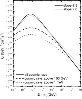
Figure 2: Contribution of cosmic rays of different energies to the hadronic $\gamma$-ray emissivity. The medium density is normalized to 1 cm^-3 and the cosmic ray spectrum is proportional to $E^{-2.3}$ (black) and $E^{-2.0}$ (grey), with an enhancement of a thousand when compared with the Earth-like one above 1 GeV. The normalization of each spectrum (of each slope) is chosen to respect the value of enhancement. In the case of the harder spectrum of $\alpha=2.0$, we show only the results for the whole cosmic ray spectrum, but a similar decrease in emissivity to that of $\alpha=2.3$ can be observed if lower energy cutoffs are imposed.

We now proceed to the computation of the $\gamma$-ray emissivity produced by a power law spectrum, with a cosmic ray enhancement of 1000 above 1 GeV. As an example, we have assumed $\alpha=2$ and $2.3$. Fig. 2 shows the results for the whole spectrum of cosmic rays (all cosmic rays, i.e., energies above 1 GeV) and for cases when the spectrum has a low energy cutoff (100 GeV and 1 TeV). For the production of secondary electrons, knock-on and pion processes need to be taken into account. Details of the computation can be found in Torres 2004. Numerical results for the knock on emissivity are shown in Fig. 3 left panel for the same spectra we have used before. If the cosmic ray spectrum is modulated, the low energy yield of knock-on electrons gets dramatically reduced. Only when the electron energies ($E_{e}$) are sufficiently large so that the minimum proton energy required to generate them ($E_{p}^{min}$) is larger than the modulation threshold, the emissivities obtained with and without modulation converge.

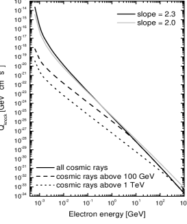
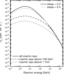
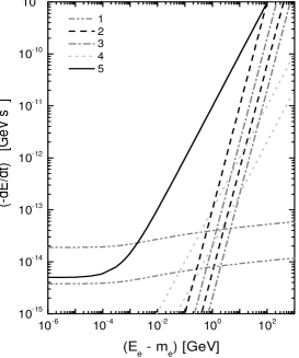
Figure 3: The effect of a modulated cosmic ray spectrum (the same as in Fig. 2 with $\alpha=2.3$ and 2.0) over the electron knock-on emissivity (left) and the positron emissivity (middle) of a medium with density $n=1$ cm^-3. Right: Different losses for assumed parameters: Curves 1 correspond to ionization losses for $n=100$ and 20 cm^-3. Curves 2 correspond to synchrotron losses for $B=50$ and 200 $\mu$G (see text). Curves 3 correspond to inverse Compton losses for a photon energy density of 20 and 100 eV cm^-3. Curves 4 correspond to Bremsstrahlung losses for $n=100$ and 20 cm^-3. Finally, curve 5 correspond to adiabatic losses having a ratio $V$(km s^-1)/$R$(pc)=300 (e.g., a wind velocity of 1500 km s^-1 and a size relevant for the escape of the electrons of 5 pc).

For the charged pion emissivity, as an example, we present numerical results for the case of positrons in Fig. 3 middle panel. As in the case of the neutral pion photon emissivity, a modulated spectrum would produce a much smaller electron and positron emissivities at relatively low energies. This difference can reach several orders of magnitude when comparing with the spectrum obtained when all cosmic rays get to interact.

4.3 Electron energy losses and distribution

Having the emissivities of secondary electrons we calculate the electron distribution solving the diffusion-loss equation. This is $\frac{N(E)}{\tau(E)}-\frac{d}{dE}\left[b(E)N(E)\right]=Q(E),$ where $Q(E)$ represents all the source terms appropriate to the production of electrons and positrons with energy $E$, $\tau(E)$ stands for the confinement timescale, $N(E)$ is the distribution of secondary particles with energies in the range $E$ and $E+dE$ per unit volume, and $b(E)=-\left({dE}/{dt}\right)$ is the rate of energy loss. The energy losses considered are those produced by ionization, inverse Compton scattering, bremsstrahlung, synchrotron radiation, and the expansion of the medium (for a compilation of the relevant formulae see the appendix in Torres 2004). A number of uncertain parameters enters into the computation of these losses. Most notably, these parameters are the medium density $n$ affecting bremsstrahlung and ionization losses, the magnetic field $B$ affecting synchrotron losses, the photon target field affecting inverse Compton losses, and the velocity of the expanding medium and the size relevant for escape, affecting the expansion losses.

Fig. 3 right panel shows the rate of energy losses for a range of parameters. We show results both $n=100$ and 20 cm^-3 and we allow magnetic fields to reach up to 200 $\mu$G in the collective wind region. The latter is made in order to fictitiously enhance –on purpose– the synchrotron losses and to better shown the dominance of the other losses mechanisms over them. Inverse Compton losses are computed using two different normalization for the energy density when the photon target is considered to be a blackbody distribution with $T_{\rm eff}$=50000 K. The expansion losses have the form

$$-\left(\frac{dE}{dt}\right)_{{\rm Adia},e}=\frac{V}{R}\left(\frac{E}{{\rm GeV}}\right){\rm GeV\;s}^{-1}\hskip 85.35826pt$$

$$=3.24\times 10^{-14}\left(\frac{V}{100\,{\rm km\;s}^{-1}}\right)\left(\frac{100{\rm pc}}{R}\right)\left(\frac{E}{{\rm GeV}}\right){\rm GeV\;s}^{-1}$$ (36)

where $V$ is the collective wind of the region, and $R$ its relevant size. In Fig. 3 right panel, to be conservative, we have chosen a ratio $V$(km s^-1)/$R$(pc)=300 (e.g., a –single or collective– wind velocity of 1500 km s^-1 and a size relevant for the escape of the electrons of 5 pc). Fig. 3 right panel shows that the expansion dominates the electron losses $b(E)$, as well as the confinement timescale $\tau(E)$, throughout a wide range of energies. In Fig. 4 we show an example of the resulting secondary electron distribution obtained by numerically solving loss equation. Only at high energies the effect of the cutoff is unnoticeable, whereas it greatly affects the production of secondaries (up to several orders of magnitude) below 10 GeV.

Figure 4: Secondary electron distribution obtained by numerically solving the loss equation. The primary cosmic ray spectrum is the same as in Fig. 2 with $\alpha=2.3$, and results are shown for different low energy cutoffs. The average density is assumed as $n=20$ cm^-3, the magnetic field is assumed as 50 $\mu$G, and the size relevant for escaping the modulating region is 5 pc. The inset shows the total energy loss rate $b(E)$.

As a benchmark, we note that the radio emission from the electron population of Fig. 4 is well below the upper limits imposed with VLA at the location of the Cygnus unidentified HEGRA source (see below for a more detailed discussion, $<200$ mJy at 1.49 GHz, Butt et al. 2003). Even assuming a rather high magnetic field of 50 $\mu$G as in Fig. 4, what is in the case of the HEGRA source discarded by X-ray and radio observations, we obtain $\sim 50$ mJy at the quoted frequency for the non-modulated cosmic ray population. A smaller magnetic field, as is probably to be found in the outer regions, or a modulated production of secondaries will diminish this estimation. We verify too that the limit is respected even when considering that the primary electron population (particularly at low energies) is at the same level than the secondary electron distribution.

4.4 Total $\gamma$-ray flux from a modulated environment

To compute $\gamma$-ray fluxes in a concrete example, and following Section 2, we consider $\sim$2 M_⊙ of target mass being modulated within $\sim$1 pc. The average density is $\sim 25$ cm^-3. This amount of mass is typical of the configurations studied in Section 2 within the innermost $20\,R_{c}\sim 2-8$ pc. To fix numerical values, we consider that the group of stars is at a Galactic distance of 2 kpc. Using the computations of secondary electrons and their distribution, the left panel of Fig. 5 shows the differential (hadronic and leptonic) $\gamma$-ray flux when the proton spectrum has a slope of 2.3 and 2.0. In the latter case, to simplify, we show only the pion decay contribution which dominates at high energies, as is produced by the whole cosmic ray spectrum.

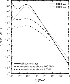
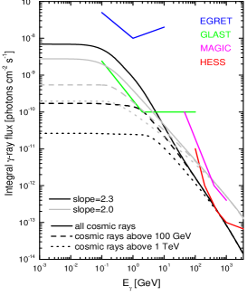
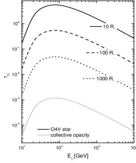
Figure 5: Differential (left) and integral (right) fluxes of $\gamma$-rays emitted in a non-modulated and a modulated environment. The bump at very low energies in the left panel is produced because we show leptonic emission coming only from secondary electrons. Above $\sim 70$ MeV the emission is dominated by neutral pion decay. Also shown are the EGRET, GLAST, MAGIC, and HESS sensitivities. Note that a source can be detectable by IACTs, and not by GLAST, or viceversa, depending on the slope of the cosmic ray spectrum and degree of modulation. Right: Opacities to $\gamma\gamma$ pair production in the soft photon field of an O4V-star at 10, 100, and 1000 $R_{\star}$, and in the collective photon field of an association with 30 stars distributed uniformly over a sphere of 0.5 pc. The closest star to the creation point is assumed to be at 0.16 pc, and the rest are placed following the average stellar density as follows: 1 additional star within 0.1, 2 within 0.25, 4 within 0.32, 8 within 0.40 and 14 within 0.5 pc.

The differential photon flux is given by $F_{\gamma}(E_{\gamma})=[{V}/{4\pi D^{2}}]{Q_{\gamma}(E_{\gamma})}=[{M}/{m_{p}\,4\pi D^{2}}][Q_{\gamma}(E_{\gamma})/n],$ where $V$ and $D$ are the volume and distance to the source, and $M$ the target mass. In those examples where the volume, distance, and/or the medium density are such that the differential flux and the integral flux obtained from it above 100 MeV with the full cosmic ray spectrum is larger than instrumental sensitivity, a modulated spectrum with a 100 GeV or a 1 TeV energy threshold might not produce a detectable source in this energy range. However, the flux will be essentially unaffected at higher energy (see the high energy end of Fig. s 2, 3, and 4). The left panel of Fig. 5 shows that wind modulation can imply that a source may be detectable for the ground-based Cerenkov telescopes without being even close to be detected by instruments in the 100 MeV – 10 GeV regime (like the late EGRET or the forthcoming GLAST). To have further insight on this, the right panel of Fig. 5 presents the integral flux of $\gamma$-rays as a function of energy, together with the sensitivity of ground-based and space-based $\gamma$-ray telescopes. The sensitivity curves shown are for point-like sources, it is expected that extended emission would require about a factor of 2 more flux to reach the same level of detectability. Table 3 summarizes these results. From Table 3 and Fig. 5 it is possible to see that there are plenty of different scenarios (possibly relevant parameters are distance, enhancement, degree of modulation of the cosmic ray spectrum, and slope) for which sources that shine enough for detection at the GLAST domain, may not do so in the IACTs energy range, and viceversa.

Table 2: Examples of results for detection in different telescopes when the configuration of collective stellar winds generates a target of about 2 M_⊙, it is located at 2 kpc, and it is bombarded with a cosmic ray spectrum having an spectral slope $\alpha=2.3$ and 2.0 enhanced a factor of $10^{3}$ above 1 GeV. The full cosmic ray spectrum and different modulated cases, at 100 GeV and 1 TeV, are shown. Except in the case of EGRET, when $\alpha=2.3$ sensitivities are barely above the expected fluxes (see Fig. (5).

Telescope	All	100 GeV	1 TeV
$\alpha=2.3$
EGRET ($E>100$ MeV)	$\times$	$\times$	$\times$
GLAST ($E>100$ MeV)	$\surd$	$\times$	$\times$
MAGIC ($E>50$ GeV)	$\times$	$\times$	$\times$
HESS/VERITAS ($E>100$ GeV)	$\times$	$\times$	$\times$
$\alpha=2.0$
EGRET ($E>100$ MeV)	$\times$	$\times$	$\times$
GLAST ($E>100$ MeV)	$\surd$	$\times$	$\times$
MAGIC ($E>300$ GeV)	$\surd$	$\surd$	$\surd$
HESS/VERITAS ($E>200$ GeV)	$\surd$	$\surd$	$\surd$

5 Opacity to $\gamma$-ray escape

The opacity to pair production of the $\gamma$-rays in the UV stellar photon field of an association can be computed as (Reimer 2003, Torres et al. 2004)

$$\tau(E_{\gamma})=\sum_{i=1}^{N}\int\int_{R_{c,i}}^{\infty}N_{i}(E_{\star})\sigma_{e^{-}e^{+}}(E_{\star},E_{\gamma})dE_{\star}dr_{i},$$ (37)

where $E_{\star}$ is the energy of the soft photons, $E_{\gamma}$ is the energy of the $\gamma$-ray, $R_{c,i}$ is the place where the photon was created with respect to the position of the star number $i$, $r_{i}$ is the distance measured from star number $i$, and $\sigma_{e^{-}e^{+}}(E_{\star},E_{\gamma})$ is the cross section for $\gamma\gamma$ pair production (Cox 1999, p.214). Note that the lower limit of the integral on $\epsilon$ in the expression for the opacity is determined from the condition that the center of mass energy of the two colliding photons should be such that $(1-(mc^{2})^{2}/(\epsilon\,E_{\gamma}))>0$. The stellar photon distribution of star number $i$ at a position $r_{i}$ from the star is that of a blackbody peaking at the star effective temperature ($T_{{\rm eff}\,i}$) and diluted by the distance factor, $N_{i}(E_{\star})=(\pi B(E_{\star}))/(hE_{\star}c)\cdot(R_{\star_{i}}^{2})/(r_{i}^{2})\,$, where $h$ is the Planck constant, $R_{\star_{i}}$ is the star number $i$ radius, and $B(E_{\star})=(2{E_{\star}}^{3})/((hc)^{2})\cdot(e^{E_{\star}/kT_{{\rm eff}\,i}}-1)^{-1}\,$.

The size of the emission region (where the target gas mass is located) that we have considered as an example in the previous sections is of the order of 1 pc. The typical radius of a massive star is 10–20 solar radius $\sim$ 5 $\times 10^{-7}$ pc, so that the most likely creation sites for photons will be far from individual stars. In Fig. 5 (right panel) we show the value of $\tau(E_{\gamma})$ for different photon creation sites distant from a O4V-star 10, 100, and 1000 $R_{\odot}$, with $R_{\star}=12R_{\odot}$ and $T_{\rm eff}=47400$ K. Unless a photon is created hovering onto the star, well within 1000 $R_{\star}$, $\gamma$-ray opacities are very low and can be safely neglected. This is still true for associations in which the number of stars is of some tens. Consider for instance a group of 30 such stars within a region of 0.5 pc (the central core of an association). The stellar density is given by Equation (1), and the number of stars within a circle of radius $R$ progresses as ${\cal N}=N(R/R_{c})^{3}$. Fig. 5 (right panel) shows the collective contribution to the opacity obtained from Equation (37) in this configuration, it is also very low since the large majority of the photons are produced far from individual stars. This, however, is not the case if one considers the collective effect of a much larger association like Cygnus OB 2, particularly at its central region (Reimer 2003). Reimer demonstrated that even when a subgroup of stars like the ones considered here is separated from a super cluster like Cygnus OB2 by about 10 pc, the influence of the latter produces an opacity about one order of magnitude larger than that produced by the local stars. Even in this case, Fig. 5 (right panel) shows that this opacity is not enough to preclude escape from the region of the local enhancement of stellar density. Such is not the case at the very center of Cygnus OB 2.

6 Candidates: Cygnus OB 2 and Westerlund 1

Extensive studies of Galactic and LMC/SMC star clusters and OB associations suggest that star formation occurs almost instantaneously (Massey et al. 1995, Leitherer 1999). Typical age spreads are about 2 Myr or less. This is short in comparison with stellar evolutionary timescales, except for the most massive stars, and so a coeval star formation seems appropriate. In addition, we are particularly interested in the case in which at the position of the stars that are being illuminated by cosmic rays there is no current star formation. If it were, the amount of gas and molecular material in the ISM would be larger than that contained in the winds, and would make the latter a subdominant contribution in the generation of the total TeV flux. In particular, should collision between cosmic rays and nuclei in the ISM be dominant, there would be no modulation. This fact and the opacity to $\gamma$-ray escape that is found in the center of a very massive cluster points to the best scenario: a sub-group of stars located in the outskirts of an association, close to an accelerator region, perhaps a SNR, or the association superbubble itself. The case of Cygnus OB 2 and the TeV source detected by HEGRA, TeV J2032+4131 (Aharonian et al. 2002, 2005b), seems to be a possible realization of this scenario. This TeV source, for which no counterparts at lower energies are presently identified (Butt et al. 2003), constant during the three years of data collection, extended (5.6$\pm 1.7$ arcmin, $\sim 2.7$ pc at 1.7 kpc), separate in about 10 pc (at 1.7 kpc) from the core of the association, and coincident with a significant enhancement of the star number density (see Fig. 1 of Butt et al. 2003) might be suggestive of the scenario outlined in the previous sections. TeV J2032+4131 presents an integral flux of about 3% of that of the Crab [$F_{\gamma}(E_{\gamma}>1$TeV$)=4.5(\pm 1.3)\times 10^{-13}$ photons cm^-2 s^-1], and a $\gamma$-ray spectrum $F_{\gamma}(E_{\gamma})=B({E_{\gamma}}/{{\rm TeV}})^{-\Gamma}$ photons cm^-2 s^-1 TeV^-1, where $B=\,4.7\,(\pm 2.1_{\rm stat}\pm 1.3_{\rm sys})\times 10^{-13}$ and $\Gamma=1.9(\pm 0.3_{\rm stat}\pm 0.3_{\rm sys}).$ Within the kind of models studied in this work, it would be possible to explain, apart from consistency with the flux level, spectrum, and variability, why there is no detectable TeV source at the central core of Cygnus OB 2 (large opacity to photon escape), and why there is no EGRET (and will not be a GLAST source) or other significant radio or X-ray diffuse emission at the position of the HEGRA detection (modulation of cosmic rays).

However, it is worth noticing that the only stars quoted by Butt et al. at the position of TeV J2032+4131 are 10 O and 10 B stars, and not even all of them are within the contours of the source. The quoted stars are similar, late O and early B, and together produce a mass-loss rate of about $1\times 10^{-5}$ M_⊙ yr^-1. This mass-loss rate is low and produces not too dense a collective wind, according to the simulations of Section 2. In addition, typical distances between these stars are of the order of a parsec, so that a central core radius is not well defined. Thus, if we are not missing significant stars in this region, something we might very well be judging on newest and deeper Chandra observations of the region (Butt et al, and Reimer et al. both in preparation) as well as on the expected star density, a better approach to study the possible contribution of stellar winds to this source is just to add that of individual stars (Torres et al. 2004). If only the currenlty known stars exist, the produced flux is too low to produce the source unless a larger enhancement or a low ISM density are invoked. A simple hadronic scenario where an enhanced spectrum interacts with more abundant ISM nuclei can not be discarded at this point, since there is no need to use modulation to explain why there is no source detected by EGRET (the predicted flux in this model is below EGRET sensitivity). However, this model can be tested with GLAST observations (see the example of Fig. 5). Also, MAGIC observations of this region are crucial. We have yet to wait for further data to reach a definitive answer.

Knödlseder (2003) has compiled a sample of massive young star clusters (Cygnus clones) that have been observed in the Galaxy (see his table 2). Westerlund 1 (Wd 1) is a prominent member. The usually adopted distance to the latter is $D\sim 1.1\pm 0.4$ kpc (Piatti et al. 1998), although Clark et al. (2005) favor a distance between 2–4 kpc. The known zoo of massive stars, clearly a lower limit in each category, includes 7 WN, 6 WC, 5 Early transition stars (like LBV, or sgB[e]) and more than 25 OB (Clark and Negueruela 2002, Clark et al. 2005). A luminous blue variable (W243) apparently undergoing an eruption event was also found (Clark & Negueruela 2004). W243’s mass-loss rate alone can be as high as $3-6\times 10^{-4}$ M_⊙ yr^-1. The stellar population of Wd 1 appears to be consistent with an age of the order 4–8 Myr if the cluster is coeval, and with a lower limit for a total mass of about a few thousand M_⊙, most likely to be around a few $\times 10^{5}$ M_⊙ (Clark & Negueruela 2002, Clark et al. 2005). Then, Wd 1 is likely to be one of the most massive young clusters in the Local Group, and in contrast to Cygnus OB2, it is much more compact (a radius of about 0.6 pc) –and thus a better target for pointing instruments. A few stars a bit far from the center (so that high opacities are avoided) subject to illumination by a cosmic ray population with a hard slope would make Wd 1 a $\gamma$-ray source. The HESS observatory has covered the position of Wd 1 when doing the galactic plane scan, although with just a few hours of observation time (Aharonian et al. 2005). We suggest that pointed observations to Wd 1 might result in its detection and that a model like the one presented here can be tested jointly by GLAST and HESS.

Finally, special interest on this model may appear in regards to the serendipitous discovered HESS J1303-631 TeV $\gamma$-ray source (Aharonian et al. 2005c), extended and still unidentified, which is in spatial coincidence with the OB association Cen OB6 (see their Fig. 7), that contain al least 20 known O stars and even 1 WR star.

7 Concluding Remarks

We have studied collective wind configurations produced by a number of massive stars, and obtained densities and expansion velocities of the stellar wind gas that is to be target for hadronic interactions in several examples. We have computed secondary particle production, electrons and positrons from charged pion decay, electrons from knock-on interactions, and solve the appropriate diffusion-loss equation with ionization, synchrotron, bremsstrahlung, inverse Compton, and expansion losses to obtain expected $\gamma$-ray emission from these regions, including in an approximate way the effect of cosmic ray modulation. Examples where different stellar configurations can produce sources for GLAST satellite, and the MAGIC/HESS/VERITAS telescopes in non-uniform ways, i.e., with or without the corresponding counterparts were shown. Finally, we have commented on Cygnus OB 2 and Westerlund 1 as two associations where this scenario could be tested. In the latter case, we have proposed it to be targeted by HESS.

Appendix: Mass loss rates and terminal velocities of individual stars

To estimate how many stars, and of what kind, are needed to get certain averages for the association parameters, we adopt the theoretical wind model C of Leitherer, Robert & Drissen (1992), where it is discussed in more detail. This model, referred to as Model THEOR in Leitherer et al. (1999), is the standard model used in the synthesis program STARBURST99 to compute spectrophotometric and statistics of starburst regions. We remark that mass-loss rates and terminal velocities are indeed uncertain (typically about $\sim 30$%). Varying the mass-loss rate and terminal velocity to those corresponding to other models will have an impact in any $\gamma$-ray luminosity computation. Alternative parameterizations to the ones below for $\dot{M}_{\star}$ and $V_{\infty}$ can be found, for instance, in the work by Vink. et al. (2000).

Table 3: Wind model parameters of WR, O, and B stars.

Stellar	$\log[\dot{M}$ ]	$V_{\infty}$
type	M⊙ yr-1	[km s-1]
WNL	-4.2	1650
WNE	-4.5	1900
WC6-9	-4.4	1800
WC4-5	-4.7	2800
WO	-5.0	3500
O3	-5.2	3190
O4	-5.4	2950
O4.5	-5.5	2900
O5	-5.6	2875
O5.5	-5.7	1960
O6	-5.8	2570
O6.5	-5.9	2455
O7	-6.0	2295
O7.5	-6.2	1975
O8	-6.3	1755
O8.5	-6.5	1970
O9	-6.7	1500
O9.5	-6.8	1500
B0	-7.0	1000
B0.5	-7.2	500
B1	-7.7	500
B1.5	-8.2	500
B2	-8.6	500
B3	-9.5	500
B5	-10.0	500
B7	-10.9	500
B8	-11.4	500
B9	-12.0	500

For WR stars, mass-loss rates are based on observations by van der Hucht et al. (1986) and Prinja et al. (1990). Average terminal velocities have been taken from Prinja (1990). For O and B stars, we shall use the parameterizations of $\dot{M}$ (M_⊙ yr^-1) and $V_{\infty}$ (km s^-1) in terms of stellar parameters (Leitehrer et al. 1992, 1999), that is also part of Model THEOR. A multidimensional fit to $\dot{M}$ (M_⊙ yr^-1) and $V_{\infty}$ (km s^-1) as a function of stellar luminosity $L$, mass $M$, effective temperature $T_{\rm eff}$, and metallicity $Z$, gives

$$\log\dot{M}({\rm M}_{\odot}\,{\rm yr}^{-1}) = -24.06+2.45\log[L({\rm L}_{\odot})]$$ (38)

$$-1.10\log[M({\rm M}_{\odot})]+1.31\log[T_{\rm eff}(K)]$$

$$+0.80\log[Z(Z_{\odot})],$$

$$V_{\infty}({\rm km\,s^{-1}}) = 1.23-0.30\log[L({\rm L}_{\odot})]+0.55\log[M({\rm M}_{\odot})]$$ (39)

$$+0.64\log[T_{\rm eff}(K)]+0.13\log[Z(Z_{\odot})].$$

In order to obtain the mass-loss rates and terminal velocities, we then need to apply a calibration between the spectral sub-types of the O and B stars and their stellar parameters. For early B and O stars we adopt the work by Vacca et al. (1996), see their Tables 5-7. Columns 2 and 3 of Table 1 show the stellar wind parameters resulting from the previous calibration. Since in general, many of the stars in a young association will pertain to luminosity class V, we give the results for this class only, although combining this Section with the work by Vacca et al. (1996), values for other classes could be obtained as needed. We adopt the values of masses as derived using evolutionary codes, since as discussed by Vacca et al. (1996), the cause of the mass discrepancy between results from the former codes and spectroscopic analysis seems to be that the models used in the spectroscopic studies do not properly take into account the effects of the wind extension, mass outflow, and velocity fields, and are thus less reliable. For B stars of late type, we complement the calibration by Vacca et al. (1996) with that of Humphreys & Mc Elroy (1984), see their Table 2, and Schmidt-Kaler (1982), which give the bolometric corrections, ($BC$), and effective temperatures. The total luminosity is then computed using the equation

$$\log(L/L_{\odot})=-0.4(M_{v}+BC-M_{\rm bol\,\odot}),$$ (40)

where $M_{\rm bol\,\odot}=4.75$ mag (Vacca et al. 1996). The masses and visual magnitudes $M_{v}$ of B stars are obtained following the method described in Appendix A of Knödlseder (2000). The star radius of each of the stars can be obtained by the usual relationship $R_{\star}^{2}=L/(4\pi\sigma T_{\rm eff}^{4})$, where $\sigma=5.67\times 10^{-5}$ erg s^-1 cm^-2 K^-4.

It is to be noted that this mass-loss parameterization may yield to an under-estimation for certain stars, and an over-estimation of the terminal velocities, like for example in the case of HD 93129A (Benaglia & Koribalski 2004). We remark that almost 400 Galactic O stars have recently been compiled in the new ‘Galactic O Star Catalogue’ (GOS) by Maíz-Apellániz & Walborn (2002), but there are only about a dozen stars known with spectral types O3.5 or earlier, thus limiting the statistical knowledge for comparison. In any case, this parameterization is enough to show that a group of several tens of early stars can easily reach a $\dot{M}_{\rm assoc}\sim{\cal O}(10^{-5}-10^{-4}$) M_⊙ yr^-1.

References

- (1) Abraham P. B., Brunstein K. A. & Cline T. L. 1966, Physical Review 150, 150
- (2) Aharonian F. 2001, Space Science Reviews 99, 187
- (3) Aharonian F. et al. 2005, Science 307, 1938
- (4) Aharonian F. et al. 2005b, A&A 431, 197
- (5) Aharonian F. et al. 2005c, A&A 439, 1013
- (6) Benaglia P. & Koribalski B. 2004, A&A 416, 171
- (7) Benaglia P., Romero G.E., Stevens I. & Torres D.F. 2001, A&A 366, 605
- (8) Bosch-Ramon V., Aharonian F. A., & Paredes J. M. (2005), A&A 432, 609 (
- (9) Bozhokin S. V. & Bykov A. M. 1994, Astronomy Letters 20, 593
- (10) Butt Y. 2003, ApJ 597, 494
- (11) Bykov, A. M., & Fleishman, G. D. 1992a, MNRAS, 255, 269
- (12) Bykov, A. M., & Fleishman, G. D. 1992b, Sov. Astron. Lett., 18, 95
- (13) Bykov, A. M. 2001, Space Sci. Rev., 99, 317
- (14) Cantó J., Raga A. C. & Rodriguez L. F. 2000, ApJ 536, 896
- (15) Castor, J., McCray, R., & Weaver, R. 1975, ApJ, L107
- (16) Chevallier R. A. & Clegg A.W. 1975, Nature 317, 44
- (17) Clark J. s. & Negueruela I. 2002, A&A 396, L25
- (18) Clark J. S. & Negueruela I. 2004, A&A 413, L15
- (19) Clark J. S., Negueruela I., Crowther P. A. & Goodwin S. P. 2005, A&A 434, 934
- (20) Cesarsky C. & Montmerle T. 1983, Space Sci. Rev. 36, 173
- (21) Cox, A. N. 1999, Allen’s Astrophysical Quantities, Springer Verlag, New York
- (22) Dermer, C. D. 1986, A&A, 157, 223
- (23) Domingo-Santamaría E. & Torres D. F. 2005, A&A, in press. astro-ph/0506240
- (24) Dorman L. 1999, Proceedings of the 26th International Cosmic Ray Conference. August 17-25, 1999. Salt Lake City, Utah, USA. Under the auspices of the International Union of Pure and Applied Physics (IUPAP). Volume 4. Edited by D. Kieda, M. Salamon, and B. Dingus, p.111
- (25) Drury, L. O’C., Aharonian, F. A., & Völk, H. J. 1994, A&A, 287, 959
- (26) GLAST Science Requirements Document, 433-SRD-0001, NASA Goddard Space Flight Center, CH-03, 2003, http://glast.gsfc.nasa.gov/project/cm/mcdl
- (27) Henrichs H. F., Schnerr R. S. & ten Kulve E. 2004, Conference Proceedings of the meeting: “The Nature and Evolution of Disks Around Hot Stars”, Johnson City, TN
- (28) Humphreys R. M. & Mc Elroy D. B. 1984, ApJ 284, 565
- (29) Jokipii, J. R., & Parker, E. N. 1970, ApJ, 160, 735
- (30) Jokipii, J. R., Kóta, J., & Merényi, E. 1993, ApJ, 405, 782
- (31) Kóta, J., & Jokipii, J. R. 1983, ApJ, 265, 573
- (32) Knödlseder J. 2000, A&A 360, 539
- (33) Knödlseder J. 2003, in ’A Massive Star Odyssey: From Main Sequence to Supernova’, Proceedings of IAU Symposium 212, held 24-28 June 2001 in Lanzarote, Canary island, Spain. Edited by Karel van der Hucht, et al. San Francisco: Astronomical Society of the Pacific, 2003., p.505
- (34) Lamers, H. J. G. L. M., & Leitherer, C. 1993, AJ, 412, 771
- (35) Lamers, H. J. G. L. M., et al. 1995, AJ, 455, 269
- (36) Lamers, H. J. G. L. M., & Cassinelli, J. P. 1999, Introduction to Stellar Winds, Cambridge University Press, Cambridge
- (37) Leitherer C., Robert C. & Drissen L. 1992, ApJ 401, 596
- (38) Leitherer C. et al. 1999, ApJ Suppl. Series 123, 3
- (39) Leitherer C. 1999, in ’Proc. of 33rd ESLAB Symp.: Star formation from the small to the large scale’ (F. Favata, A. A. Kaas & A. Wilson eds., ESA SP-445, 2000)
- (40) Maíz-Apellániz, J., & Walborn, N. R. 2002, in “A Massive Star Odyssey: from Main Sequence to Supernova”, eds. K. A. van der Hucht, A. Herrero, & C. Esteban, ASP Conf. Ser. 212, p. 560
- (41) Manchanda R. K. et al. 1996, A&A 305, 457
- (42) Massey, P., Johnson, K. E., & DeGioia-Eastwood, K. 1995, ApJ, 454, 151
- (43) Ozernoy L. M., Genzel R. & Usov V. 1997, MNRAS 288, 237
- (44) Parker E. M. 1958, Phys. Rev., 110, 1445
- (45) Prinja, R. K., et al. 1990, AJ, 361, 607
- (46) Parizot E. et al. 2004, A&A 424, 727
- (47) Reimer A. 2003, Proceedings of the 28th International Cosmic Ray Conference, p.2505
- (48) Romero, G. E., Benaglia, P., & Torres, D. F. 1999, A&A, 348, 868
- (49) Schmidt-Kaler Th., 1982, Landolt-Börnstein Vol. 2
- (50) Smith L. F., Maeder A., 1991, A&A, 241, 77
- (51) Stevens I. R. & Hartwell J. M. 2003, MNRAS 339, 280
- (52) Torres, D. F. 2004, ApJ 617, 966
- (53) Torres D. F., Romero G. E., Dame T. M., Combi J. A. & Butt Y. M. 2003, Physics Reports 382, 303
- (54) Torres D. F., Reimer O., Domingo-Santamaría E. & Digel S. 2004, ApJ 607, L99
- (55) Torres, D. F., Domingo-Santamaría, E., & Romero, G. E. 2004, ApJ 601, L75
- (56) Vacca, W.D., Garmany, C.D., Schull, J.M. 1996, ApJ 460, 914
- (57) Van der Hucht 1986., et al. 1996, AJ, 460, 914
- (58) Völk, H. J., & Forman, M. 1982, ApJ, 253, 188
- (59) Völk H., Aharonian F. A. & Breitschwerdt D. 1996, Space Science Reviews 75, 279
- (60) Weber, E. J., & Davis, L. 1967, ApJ, 148, 217
- (61) White, R. L. 1985, ApJ, 289, 698