PARTICLE DIFFUSION AND ACCELERATION BY SHOCK WAVE IN MAGNETIZED FILAMENTARY TURBULENCE

Abstract

We expand the off-resonant scattering theory for particle diffusion in magnetized current filaments that can be typically compared to astrophysical jets, including active galactic nucleus jets. In a high plasma $\beta$ region where the directional bulk flow is a free-energy source for establishing turbulent magnetic fields via current filamentation instabilities, a novel version of quasi-linear theory to describe the diffusion of test particles is proposed. The theory relies on the proviso that the injected energetic particles are not trapped in the small-scale structure of magnetic fields wrapping around and permeating a filament but deflected by the filaments, to open a new regime of the energy hierarchy mediated by a transition compared to the particle injection. The diffusion coefficient derived from a quasi-linear type equation is applied to estimating the timescale for the stochastic acceleration of particles by the shock wave propagating through the jet. The generic scalings of the achievable highest energy of an accelerated ion and electron, as well as of the characteristic time for conceivable energy restrictions, are systematically presented. We also discuss a feasible method of verifying the theoretical predictions. The strong, anisotropic turbulence reflecting cosmic filaments might be the key to the problem of the acceleration mechanism of the highest energy cosmic rays exceeding $100~{}{\rm EeV}$ ($10^{20}~{}{\rm eV}$), detected in recent air shower experiments.

1 INTRODUCTION

Extremely high energy (EHE) cosmic rays beyond $100~{}{\rm EeV}$ have been observed in a couple of decades (Takeda et al., 1998; Abbasi et al., 2004a), but their origin still remains enigmatic. In regard to the generation of the EHE particles, there are two alternative schemes: the “top-down” scenario that hypothesizes topological defects, Z-bursts, and so on, and the traditional “bottom-up” (see, e.g., Olinto, 2000, for a review). In the latter approach, we explore the candidate celestial objects operating as a cosmic-ray “Zevatron” (Blandford, 2000), namely, an accelerator boosting particle kinetic energy to ZeV ($10^{21}~{}{\rm eV}$) ranges. By simply relating the celestial size to the gyroradius for the typical magnetic field strength, one finds that the candidates are restricted to only a few objects; these include pulsars, active galactic nuclei (AGNs), radio galaxy lobes, and clusters of galaxies (Hillas, 1984; Olinto, 2000). In addition, gamma-ray bursters (GRBs) are known as possible sources (Waxman, 1995). As for the transport of EHE particles from the extragalactic sources, within the GZK horizon (Greisen, 1966; Zatsepin & Kuzmin, 1966) the trajectory of the particles (particularly protons) ought to suffer no significant deflection due to the cosmological magnetic field, presuming its strength of the order of $0.1~{}{\rm nG}$ (see, e.g., Vallée, 2004, for a review). According to a cross-correlation study (Farrar & Biermann, 1998), some super-GZK events seem to be well aligned with compact, radio-loud quasars. Complementarily, self-correlation study is in progress, showing small-scale anisotropy in the distribution of the arrival direction of EHE primaries (Teshima et al., 2003). More recently, the strong clustering has been confirmed, as is consistent with the null hypothesis of isotropically distributed arrival directions (Abbasi et al., 2004b). At the moment, the interpretation of these results is under active debate.

In the bottom-up scenario, the most promising mechanism for achieving EHE is considered to be that of diffusive shock acceleration (DSA; Lagage & Cesarsky, 1983a, b; Drury, 1983), which has been substantially studied for solving the problems of particle acceleration in heliosphere and supernova remnant (SNR) shocks (see, e.g., Blandford & Eichler, 1987, for a review). In general, it calls for the shock to be accompanied by some kinds of turbulence that serve as the particle scatterers (Krymskii, 1977; Bell, 1978; Blandford & Ostriker, 1978). Concerning the theoretical modeling and its application to extragalactic sources such as AGN jets, GRBs, and so forth, it is still very important to know the actual magnetic field strength, configuration, and turbulent state around the shock front. At this juncture, modern polarization measurements by using very long baseline interferometry began to reveal the detailed configuration of magnetic fields in extragalactic jets, for example, the quite smooth fields transverse to the jet axis (1803+784: Gabuzda, 1999). Another noticeable result is that within the current resolution, a jet is envisaged as a bundle of at least a few filaments (e.g., 3C 84: Asada et al. 2000; 3C 273: Lobanov & Zensus 2001), as were previously confirmed in the radio arcs near the Galactic center (GC; Yusef-Zadeh et al., 1984; Yusef-Zadeh & Morris, 1987), as well as in the well-known extragalactic jets (e.g., Cyg A: Perley et al. 1984, Carilli & Barthel 1996; M87: Owen et al. 1989).

The morphology of filaments can be self-organized via the nonlinear development of the electromagnetic current filamentation instability (CFI; Honda, 2004, and references therein) that breaks up a uniform beam into many filaments, each carrying about net one unit current (Honda, 2000). Fully kinetic simulations indicated that this subsequently led to the coalescence of the filaments, self-generating significant toroidal (transverse) components of magnetic fields (Honda et al., 2000a, b). As could be accommodated with this result, large-scale toroidal magnetic fields have recently been discovered in the GC region (Novak et al., 2003). Accordingly, we conjecture that a similar configuration appears in extragalactic objects, particularly AGN jets (Honda & Honda, 2004a). It is also pointed out that the toroidal fields could play a remarkable role in collimating plasma flows (Honda & Honda, 2002). Relating to this point, the AGN jets have narrow opening angles of $\phi_{\rm oa}<10\arcdeg$ in the long scales, although in close proximity to the central engine the angles tend to spread (e.g., $\phi_{\rm oa}\approx 60\arcdeg$ for the M87 jet; Junor et al., 1999). Moreover, there is observational evidence that the internal pressures are higher than the pressures in the external medium (e.g., 4C 32.69: Potash & Wardle 1980; Cyg A: Perley et al. 1984; M87: Owen et al. 1989). These imply that the jets must be self-collimating and stably propagating, as could be explained by the kinetic theory (Honda & Honda, 2002).

In the nonlinear stage of the CFI, the magnetized filaments can often be regarded as strong turbulence that more strongly deflects the charged particles. When the shock propagation is allowed, hence, the particles are expected to be quite efficiently accelerated for the DSA scenario (Drury, 1983; Gaisser, 1990). Indeed, such a favorable environment seems to be well established in the AGN jets. For example, in the filamentary M87 jet, some knots moving toward the radio lobe exhibit the characteristics of shock discontinuity (Biretta et al., 1983; Capetti et al., 1997), involving circumstantial evidence of in situ electron acceleration (Meisenheimer et al., 1996). As long as the shock accelerator operates for electrons, arbitrary ions will be co-accelerated, providing that the ion abundance in the jet is finite (e.g., Rawlings & Saunders, 1991; Kotani et al., 1996). It is, therefore, quite significant to study the feasibility of EHE particle production in the filamentary jets with shocks: this is just the original motivation for the current work.

This paper has been prepared to show a full derivation of the diffusion coefficient for cosmic-ray particles scattered by the magnetized filaments. The present theory relies on a consensus that the kinetic energy density (ram pressure) of the bulk plasma carrying currents is larger than the energy density of the magnetic fields self-generated via the CFI, likely comparable to the thermal pressure of the bulk. That is, the flowing plasma as a reservoir of free energy is considered to be in a high-$\beta$ state. In a new regime in which the cosmic-ray particles interact off-resonantly with the magnetic turbulence having no regular field, the quasi-linear approximation of the kinetic transport equation is found to be consistent with the condition that the accelerated particles must be rather free from magnetic traps; namely, the particles experience meandering motion. It follows that the diffusion anisotropy becomes small. Apparently, these are in contrast with the conventional quasi-linear theory (QLT) for small-angle resonant scattering, according to which one sets the resonance of the gyrating particles bound to a mean magnetic field with the weak turbulence superimposed on the mean field (Drury, 1983; Biermann & Strittmatter, 1987; Longair, 1992; Honda & Honda, 2004b). It is found that there is a wide parameter range in which the resulting diffusion coefficient is smaller than that from a simplistic QLT in the low-$\beta$ regime. We compare a specified configuration of the filaments to an astrophysical jet including AGN jets and discuss the correct treatment of what the particle injection threshold in the present context could be. We then apply the derived coefficient for calculations of the DSA timescale and the achievable highest energy of accelerated particles in that environment. As a matter of convenience, we also show some generic scalings of the highest energy, taking account of the conceivable energy restrictions for both ions and electrons.

In order to systematically spell out the theoretical scenario, this paper is divided into two major parts, consisting of the derivation of the diffusion coefficient (§ 2) and its installation to the DSA model (§ 3). We begin, in § 2.1, with a discussion on the turbulent excitation mechanism due to the CFI, so as to specify a model configuration of the magnetized current filaments. Then in § 2.2, we explicitly formulate the equation that describes particle transport in the random magnetic fluctuations. In § 2.3, the power-law spectral index of the magnetic fluctuations is suggested for a specific case. In § 2.4, we write down the diffusion coefficients derived from the transport equation. In § 3.1, we deal with the subject of particle injection, and in § 3.2, we estimate the DSA timescale, which is used to evaluate the maximum energy of an accelerated ion (§ 3.3) and electron (§ 3.4). Finally, § 4 is devoted to a discussion of the feasibility and a summary.

2 THEORY OF PARTICLE DIFFUSION IN MAGNETIC TURBULENCE SUSTAINED BY ANISOTROPIC CURRENT FILAMENTS

In what follows, given the spatial configuration of the magnetized filaments of a bulk plasma jet, we derive the evolution equation for the momentum distribution function of test particles, which is linear to the turbulent spectral intensity, and then extract an effective frequency for collisionless scattering and the corresponding diffusion coefficient from the derived equation.

2.1 Model Configuration of Magnetized Current Filaments

Respecting the macroscopic transport of energetic particles in active galaxies, there is direct/indirect observational evidence that they are ejected from the central core of the galaxies and subsequently transferred, through bipolar jets, to large-scale radio robes in which the kinematic energy considerably dissipates (e.g., Biretta et al., 1995; Tashiro & Isobe, 2004). In this picture, it is expected that the directional plasma flows will favorably induce huge currents in various aspects of the above transport process (e.g., Appl & Camenzind 1992; Conway et al. 1993; an analogous situation also seems to appear in GRB jets: e.g., Lyutikov & Blandford 2003). Because of perfect conductivity in fully ionized plasmas, hot currents driven in, e.g., the central engine prefer being quickly compensated by plasma return currents. This creates a pattern of the counterstreaming currents that is unstable for the electromagnetic CFI. As is well known, the pattern is also unstable to electrostatic disturbances with the propagation vectors parallel to the streaming direction, but in the present work, we eliminate the longitudinal modes, so as to isolate the transverse CFI. Providing a simple case in which the two uniform currents are carried by electrons, the mechanism of magnetic field amplification due to the CFI is explained as follows. When the compensation of the counterpropagating electron currents is disturbed in the transverse direction, magnetic repulsion between the two currents reinforces the initial disturbance. As a consequence, a larger and larger magnetic field is produced as time increases. For the Weibel instability as an example, the unstable mode is the purely growing mode without oscillations (Honda, 2004), so the temporal variation of magnetic fields is expected to be markedly slow in the saturation regime (more on these is given in §§ 2.2 and 2.3). Note that a similar pattern of quasi-static magnetic fields can be also established during the collision of electron-positron plasmas (Kazimura et al., 1998; Silva et al., 2003) and in a shock front propagating through an ambient plasma with/without initial magnetic fields (Nishikawa et al., 2003). These dynamics might be involved in the organization of the knotlike features in the Fanaroff-Riley (FR) type I radio jets, which appear to be a shock caused by high-velocity material overtaking slower material (e.g., Biretta et al., 1983). Similarly, the cumulative impingement could also take place around the hot spots of the FR type II sources, which arguably reflect the termination shocks. In fact, the filamentary structure has been observed in the hot spot region of a FR II source (Perley et al., 1984; Carilli & Barthel, 1996).

Furthermore, estimating the energy budget in many radio lobes implies that the ram pressure of such current-carrying jets is much larger than the energy density of the magnetic fields (Tashiro & Isobe, 2004); namely, the jet bulk can be regarded as a huge reservoir of free energy. In this regime, the ballistic motion is unlikely to be affected by the self-generated magnetic fields, as is actually seen in the linear feature of jets. As a matter of fact, the GC region is known to arrange numerous linear filaments, including nonthermal filaments (Yusef-Zadeh et al., 2004).

Taking these into consideration, we give a simple model of the corresponding current–magnetic field system and attempt to unambiguously distinguish the present system from the one that appears in the low-$\beta$ plasmas hitherto well studied. In Figure 1, for a given coordinate, we depict the configuration of the linear current filaments and turbulent magnetic fields of the bulk plasma. Recalling that magnetic field perturbations develop in the direction transverse to the initial currents (e.g., Honda, 2004), one supposes the magnetic fields developed in the nonlinear phase to be ${\bf B}=(B_{x},B_{y},0)$ (Montgomery & Liu, 1979; Medvedev & Loeb, 1999), such that the vectors of zeroth-order current density point in the directions parallel and antiparallel to the $z$-direction, i.e., ${\bf J}\sim J{\hat{\bf z}}$, where the scalar $J$ ($\gtrless 0$) is nonuniformly distributed on the transverse $x$-$y$ plane, while uniformly distributed in the $z$-direction. Note that for the fluctuating magnetic field vectors, we have used the simple character (${\bf B}$) without any additional symbol such as “$\delta$,” since the establishment of no significant regular component is expected, and simultaneously, ${\bf J}$ ($\sim\nabla\times{\bf B}$) well embodies the quasi-static current filaments in the zeroth order. For convenience, hereafter, the notations “parallel” ($\parallel$) and “transverse” ($\perp$) are referred to as the directions with respect to the linear current filaments aligned in the $z$-axis, as they are well defined reasonably (n.b. in the review of § 2.4, $\parallel_{b}$ and $\perp_{b}$ with the subscript “$b$” refer to a mean magnetic field line). It is mentioned that the greatly fluctuating transverse fields could be reproduced by some numerical simulations (e.g., Lee & Lampe, 1973; Nishikawa et al., 2003). In an actual filamentary jet, a significant reduction of polarization has been found in the center, which could be ascribed to the cancellation of the small-scale structure of magnetic fields (Capetti et al., 1997), compatible with the present model configuration. In addition, there is strong evidence that random fields accompany GRB jets (e.g., Greiner et al., 2003). The arguments expanded below highlight the transport properties of test particles in such a bulk environment, that is, in a forest of magnetized current filaments.

2.2 The Quasi-linear Type Equation for Cosmic-Ray Transport

We are particularly concerned with the stochastic diffusion of the energetic test particles injected into the magnetized current filaments (for the injection problem, see the discussion in § 3.1). As a rule, the Vlasov equation is appropriate for describing the collisionless transport of the relativistic particles in the turbulent magnetic field, ${\bf B}({\bf r},t)$, where ${\bf r}=(x,y)$ and the slow temporal variation has been taken into consideration. Transverse electrostatic fields are ignored, since they preferentially attenuate over long timescales, e.g., in the propagation time of jets (see § 2.3). The temporal evolution of the momentum distribution function for the test particles, $f_{\bf p}$, can then be described as

$${{\rm D}f_{\bf p}\over{{\rm D}t}}={\partial\over{\partial t}}f_{\bf p}+\left({\bf v}\cdot{\partial\over{\partial{\bf r}}}\right)f_{\bf p}+{q\over c}\left[\left({\bf v}\times{\bf B}\right)\cdot{\partial\over{\partial{\bf p}}}\right]f_{\bf p}=0$$ (1)

for arbitrary particles. Here $q$ is the particle charge, $c$ is the speed of light, and the other notations are standard. We decompose the total distribution function into the averaged and fluctuating part, $f_{\bf p}=\left<f_{\bf p}\right>+\delta f_{\bf p}$, and consider the specific case in which from a macroscopic point of view, the vector ${\bf B}=(B_{x},B_{y},0)$ is randomly distributed on the transverse $x$-$y$ plane (Montgomery & Liu, 1979; Medvedev & Loeb, 1999). Taking the ensemble average of equation (1), $\left<{\rm D}f_{\bf p}/{{\rm D}t}\right>=0$, then yields

$${\partial\over{\partial t}}\left<f_{\bf p}\right>+\left({\bf v}\cdot{\partial\over{\partial{\bf r}}}\right)\left<f_{\bf p}\right>=-{q\over c}\left<\left[\left({\bf v}\times{\bf B}\right)\cdot{\partial\over{\partial{\bf p}}}\right]\delta f_{\bf p}\right>,$$ (2)

where we have used $\left<{\bf B}\right>\simeq{\bf 0}$. Taking account of no mean field implies that we do not invoke the gyration and guiding center motion of the particles. Subtracting equation (2) from equation (1) and picking up the term linear in fluctuations, viz., employing the conventional quasi-linear approximation, we obtain

$${\partial\over{\partial t}}\delta f_{\bf p}+\left({\bf v}\cdot{\partial\over{\partial{\bf r}}}\right)\delta f_{\bf p}=-{q\over c}\left[\left({\bf v}\times{\bf B}\right)\cdot{\partial\over{\partial{\bf p}}}\right]\left<f_{\bf p}\right>.$$ (3)

As usual, equation (3) is valid for $\left<f_{\bf p}\right>\gg|\delta f_{\bf p}|$ (Landau & Lifshitz, 1981). As shown in § 3.1, this condition turns out to be consistent with the aforementioned implication that the injected test particles must be free from the small-scale magnetic traps embedded in the bulk. Relating to this, note that to remove the ambiguity of terminologies, the injected, energetic test particles obeying $f_{\bf p}$ are just compared to the cosmic rays that are shown below to be diffusively accelerated owing to the present scenario. Within the framework of the test particle approximation, the back-reaction of the slow spatiotemporal change of $\left<f_{\bf p}\right>$ to the modulation of ${\bf B}$ (sustained by the bulk) is ignored, in contrast to the case for SNR environments, where such effects often become nonnegligible (e.g., Bell, 2004).

In general, the vector potential conforms to ${\bf B}=\nabla\times{\bf A}$ and $\nabla\cdot{\bf A}=0$. For the standard, plane wave approximation, we carry out the Fourier transformation of the fluctuating components for time and the transverse plane:

$$\delta f_{\bf p}({\bf r},t)=\int\delta f_{{\bf p},{\cal K}}e^{i\left[\left({\bf k}\cdot{\bf r}\right)-\omega t\right]}{\rm d}^{3}{\cal K},$$ (4)

$${\bf A}({\bf r},t)=\int{\bf A}_{\cal K}e^{i\left[\left({\bf k}\cdot{\bf r}\right)-\omega t\right]}{\rm d}^{3}{\cal K},$$ (5)

$${\bf B}({\bf r},t)=\int{\bf B}_{\cal K}e^{i\left[\left({\bf k}\cdot{\bf r}\right)-\omega t\right]}{\rm d}^{3}{\cal K},$$ (6)

and ${\bf B}_{\cal K}=i{\bf k}\times{\bf A}_{\cal K}$, where $i=\sqrt{-1}$, ${\cal K}=\left\{{\bf k},\omega\right\}$, and ${\rm d}^{3}{\cal K}={\rm d}^{2}{\bf k}{\rm d\omega}$. The given magnetic field configuration follows ${\bf A}=A{\hat{\bf z}}$ (${\bf A}_{\cal K}=A_{\cal K}{\hat{\bf z}}$) and ${\bf k}\perp{\hat{\bf z}}$. As illustrated in Figure 1, the scalar quantity $A$ ($\gtrless 0$) is also random on the transverse plane, with no mean value. Making use of equations (4)–(6), equation (3) can be transformed into

$$\delta f_{{\bf p},{\cal K}}={q\over c}\left[\omega-\left({\bf k}\cdot{\bf v}\right)\right]^{-1}\left[{\bf v}\times\left({\bf k}\times{\bf A}_{\cal K}\right)\right]\cdot{{\partial\left<f_{\bf p}\right>}\over{\partial{\bf p}}}.$$ (7)

On the other hand, the right-hand side (RHS) of equation (2) can be written as

$${\rm RHS}=-i{q\over c}\left<\int{\rm d}^{3}{\cal K}^{\prime}e^{i\left[\left({\bf k}^{\prime}\cdot{\bf r}\right)-\omega^{\prime}t\right]}\left\{\left[{\bf v}\times\left({\bf k}^{\prime}\times{\bf A}_{{\cal K}^{\prime}}\right)\right]\cdot{\partial\over{\partial{\bf p}}}\right\}\delta f_{\bf p}\right>.$$ (8)

Substituting equation (4) (involving eq. [7]) into equation (8), equation (2) can be expressed as

$${{{\rm d}\left<f_{\bf p}\right>}\over{{\rm d}t}}=-i{q^{2}\over c^{2}}\left<\int{\rm d}^{3}{\cal K}{\rm d}^{3}{\cal K}^{\prime}e^{i\left\{\left[\left({\bf k}+{\bf k}^{\prime}\right)\cdot{\bf r}\right]-\left(\omega+\omega^{\prime}\right)t\right\}}\right.$$

$$\left.\left[{\bf v}\times\left({\bf k}^{\prime}\times{\bf A}_{{\cal K}^{\prime}}\right)\right]\cdot{\partial\over{\partial{\bf p}}}\left\{{{\left[{\bf v}\times\left({\bf k}\times{\bf A}_{\cal K}\right)\right]}\over{\omega-\left({\bf k}\cdot{\bf v}\right)}}\cdot{\partial\over{\partial{\bf p}}}\right\}\left<f_{\bf p}\right>\right>,$$ (9)

where the definition of the total derivative, ${\rm d}/{\rm d}t\equiv\partial/{\partial t}+{\bf v}\cdot\left({\partial/{\partial{\bf r}}}\right)$, has been introduced. As for the integrand of equation (9), it may be instructive to write down the vector identity of

$${\bf v}\times\left({\bf k}^{(\prime)}\times{\bf A}_{{\cal K}^{(\prime)}}\right)=\left({\bf v}\cdot{\bf A}_{{\cal K}^{(\prime)}}\right){\bf k}^{(\prime)}-\left({\bf k}^{(\prime)}\cdot{\bf v}\right){\bf A}_{{\cal K}^{(\prime)}}.$$ (10)

From the general expression of equation (9), we derive an effective collision frequency that stems from fluctuating field-particle interaction, as shown below.

For convenience, we decompose the collision integral (RHS of eq. [9]) including the scalar products, $\cdot\left(\partial/\partial{\bf p}\right)$, into the four parts:

$${{{\rm d}\left<f_{\bf p}\right>}\over{{\rm d}t}}=\sum_{i,j}I_{ij},$$ (11)

where $i,j=1,2$ and

$$I_{ij}\equiv-i{q^{2}\over c^{2}}\left<\int{\rm d}^{3}{\cal K}{\rm d}^{3}{\cal K}^{\prime}\cdots{\partial\over{\partial p_{i}}}\cdots{\partial\over{\partial p_{j}}}\left<f_{\bf p}\right>\right>.$$ (12)

In the following notations, the subscripts “1” and “2” indicate the parallel ($\parallel$) and perpendicular ($\perp$) direction to the current filaments, respectively. Below, as an example, we investigate the contribution from the integral $I_{11}$ (see Appendix for calculation of the other components). For the purely parallel diffusion involving the partial derivative of only $\partial/\partial p_{\parallel}$, the first term of the RHS of equation (10) does not make a contribution to equation (9).

In the ordinary case in which the random fluctuations are stationary and homogeneous, the correlation function has its sharp peak at $\omega=-\omega^{\prime}$ and ${\bf k}=-{\bf k}^{\prime}$ (Tsytovich & ter Haar, 1995), that is,

$$\left<A_{\cal K}A_{{\cal K}^{\prime}}\right>=|A|_{{\bf k},\omega}^{2}\delta({\bf k}+{\bf k}^{\prime})\delta(\omega+\omega^{\prime}),$$ (13)

where the Dirac $\delta$-function has been used. Here note the relation of $|A|_{{\bf k},\omega}^{2}=|A|_{{\bf-k},-\omega}^{2}$ because we have $A_{{\bf-k},-\omega}=A_{{\bf k},\omega}^{*}$, where the superscript asterisk indicates the complex conjugate; this is valid as far as ${\bf A}({\bf r},t)$ is real, i.e., ${\bf B}({\bf r},t)$ is observable. By using equation (13), the integral component $I_{11}$ can be expressed as

$$I_{11}=i{q^{2}\over c^{2}}\int{\rm d}^{2}{\bf k}{\rm d}\omega|A|_{{\bf k},\omega}^{2}\left({\bf k}\cdot{\bf v}\right){\partial\over{\partial p_{\parallel}}}\left[{{{\bf k}\cdot{\bf v}}\over{\omega-\left({\bf k}\cdot{\bf v}\right)}}{\partial\over{\partial p_{\parallel}}}\left<f_{\bf p}\right>\right],$$ (14)

where the relation of ${\bf A}_{\cal K}\cdot\left(\partial/\partial{\bf p}\right)=A_{\cal K}\left(\partial/\partial p_{\parallel}\right)$ has been used. In order to handle the resonant denominator of equation (14), we introduce the causality principle of $\lim_{\epsilon\rightarrow+0}\left[\omega-\left({\bf k}\cdot{\bf v}\right)+i\epsilon\right]^{-1}\rightarrow{\cal P}\left[\omega-\left({\bf k}\cdot{\bf v}\right)\right]^{-1}-i\pi\delta\left[\omega-\left({\bf k}\cdot{\bf v}\right)\right]$, where ${\cal P}$ indicates the principal value (Landau & Lifshitz, 1981). One can readily confirm that the real part of the resonant denominator does not contribute to the integration. Thus, we have

$$I_{11}={{\pi q^{2}}\over c^{2}}\int{\rm d}^{2}{\bf k}{\rm d}\omega|A|_{{\bf k},\omega}^{2}\left({\bf k}\cdot{\bf v}\right){\partial\over{\partial p_{\parallel}}}\left\{\delta\left[\omega-\left({\bf k}\cdot{\bf v}\right)\right]\left({\bf k}\cdot{\bf v}\right){\partial\over{\partial p_{\parallel}}}\left<f_{\bf p}\right>\right\}.$$ (15)

Equation (15) shows the generalized form of the quasi-linear equation, allowing $|A|_{{\bf k},\omega}^{2}$ to be arbitrary functions of ${\bf k}$ and $\omega$. In the present circumstances, a typical unstable mode of the CFI is the purely growing Weibel mode with $\omega=0$ in collisionless regimes, although in a dissipative regime the dephasing modes with a finite but small value of $\omega=\pm\Delta\omega_{\bf k}$ are possibly excited (Honda, 2004). In the latter case, the spectral lines will be broadened in the nonlinear phase. Nevertheless, it is assumed that the spectrum still retains the peaks around $\omega\approx\pm\Delta\omega$, accompanied by their small broadening of the same order, where $|\Delta\omega|\ll\gamma_{\bf k}\sim\omega_{\rm p}$, and $\gamma_{\bf k}$ and $\omega_{\rm p}/(2\pi)$ are the growth rate and the plasma frequency, respectively. In the special case reflecting the purely growing mode, the spectrum retains a narrow peak at $\omega=0$ with $|\Delta\omega|\sim 0$ (Montgomery & Liu, 1979). Apparently, the assumed quasi-static properties are in accordance with the results of the fully kinetic simulations (Kazimura et al., 1998; Honda et al., 2000a), except for a peculiar temporal property of the rapid coalescence of filaments. Accordingly, here we employ an approximate expression of

$$|A|_{{\bf k},\omega}^{2}\sim|A|_{\bf k}^{2}\delta\left(\omega-\Delta\omega\right)+|A|_{\bf-k}^{2}\delta\left(\omega+\Delta\omega\right),$$ (16)

where $|A|_{\bf k}^{2}=|A|_{\bf-k}^{2}$. Note that when taking the limit of $|\Delta\omega|\rightarrow 0$, equation (16) degenerates into $|A|_{{\bf k},\omega}^{2}\sim 2|A|_{\bf k}^{2}\delta\left(\omega\right)$.

Substituting equation (16) into equation (15) yields

$$I_{11}\sim{{2\pi q^{2}}\over c^{2}}\int{\rm d}^{2}{\bf k}|A|_{\bf k}^{2}\left({\bf k}\cdot{\bf v}\right){\partial\over{\partial p_{\parallel}}}\left\{\delta\left[\Delta\omega-\left({\bf k}\cdot{\bf v}\right)\right]\left({\bf k}\cdot{\bf v}\right){\partial\over{\partial p_{\parallel}}}\left<f_{\bf p}\right>\right\}.$$ (17)

Furthermore, we postulate that the turbulence is isotropic on the transverse plane, though still, of course, allowing anisotropy of the vectors ${\bf A}$ parallel to the $z$-axis. Equation (17) can be then cast to

$$I_{11}\sim{{2\pi q^{2}}\over c^{2}}v_{\perp}{\partial\over{\partial p_{\parallel}}}\int{{\rm d}\theta\over{2\pi}}\cos^{2}\theta\int{\rm d}k2\pi k\delta\left(\Delta\omega-kv_{\perp}\cos\theta\right){k^{2}|A|_{k}^{2}}v_{\perp}{\partial\over{\partial p_{\parallel}}}\left<f_{\bf p}\right>,$$ (18)

where $k=|{\bf k}|$, $v_{\perp}=|{\bf v}_{\perp}|$, and ${\bf k}\cdot{\bf v}={\bf k}\cdot\left({\bf v}_{\perp}+v_{\parallel}{\hat{\bf z}}\right)=kv_{\perp}\cos\theta$.

As concerns the integration for $\theta$, we see that the contribution from the marginal region of the smaller $|\cos\theta|$, reflecting narrower pitch angle, is negligible. In astrophysical jets, the pitch angle distribution for energetic particles still remains unresolved, although the distribution itself is presumably unimportant. Hence, at the moment it may be adequate to simply take an angular average, considering, for heuristic purposes, the contribution from the range of $|\cos\theta|\sim O(1)\gg\epsilon$ for a small value of $\epsilon$. If one can choose $\epsilon\gtrsim|\Delta\omega|/(k_{\rm min}v_{\perp})$, the above relation, $\epsilon\ll|\cos\theta|$, reflects the off-resonant interaction, i.e., $|\Delta\omega|\ll|{\bf k}\cdot{\bf v}|$. The minimum wavenumber, $k_{\rm min}$, is typically of the order of the reciprocal of the finite system size, which is, in the present circumstances, larger than the skin depth $c/\omega_{\rm p}$. These ensure the aforementioned relation of $|\Delta\omega|\ll\omega_{\rm p}$ (or $|\Delta\omega|\sim 0$). In addition, the off-resonance condition provides an approximate expression of $\delta\left(\Delta\omega-kv_{\perp}\cos\theta\right)\sim\left(kv_{\perp}|\cos\theta|\right)^{-1}$. Using this expression, the integral for the angular average can be approximated by $\sim\int_{0}^{2\pi}\cos^{2}\theta/(2\pi|\cos\theta|){\rm d}\theta=2/\pi$. This is feasible, on account of the negligible contribution from the angle of $|\cos\theta|\lesssim\epsilon$. Then equation (18) reduces to

$$I_{11}\sim{{16\pi q^{2}}\over c^{2}}v_{\perp}{\partial^{2}\over{\partial p_{\parallel}^{2}}}\left<f_{\bf p}\right>\int_{k_{\rm min}}^{k_{\rm max}}{{{\rm d}k}\over k}I_{k},$$ (19)

where we have defined the modal energy density (spectral intensity) of the quasi-static turbulence by $I_{k}\equiv 2\pi k\left(k^{2}|A|_{k}^{2}/4\pi\right)$, such that the magnetic energy density in the plasma medium can be evaluated by $u_{\rm m}\simeq\left<|{\bf B}|^{2}\right>/8\pi=\int_{k_{\rm min}}^{k_{\rm max}}I_{k}{\rm d}k$.

2.3 Spectral Intensity of the Transverse Magnetic Fields

The energy density of the quasi-static magnetic fields, $u_{\rm m}$, likely becomes comparable to the thermal pressure of the filaments (Honda et al., 2000a, b; Honda & Honda, 2002). When exhibiting such a higher $u_{\rm m}$ level, the bulk plasma state may be regarded as the strong turbulence; but recall that in the nonlinear CFI, the frequency spectrum with a sharp peak at $\omega=0$ is scarcely smoothed out, since significant mode-mode energy exchanges are unexpected. This feature is in contrast to the ordinary magnetohydrodynamic (MHD) and electrostatic turbulence, in which a larger energy density of fluctuating fields would involve modal energy transfer. One of the most remarkable points is that as long as the validity condition of the quasi-linear approximation, $\left<f_{\bf p}\right>\gg|\delta f_{\bf p}|$, is satisfied (for details, see § 3.1), the present off-resonant scattering theory covers even the strong turbulence regime. That is, the theory, which might be classified into an extended version of the QLT, does not explicitly restrict the magnetic turbulence to be weak (for instruction, Tsytovich & ter Haar [1995] have considered a generalization of the quasi-linear equation in regard to its application to strong electrostatic turbulence). Apparently, this is also in contrast to the conventional QLT for small-angle resonant scattering, which invokes a mean magnetic field (well defined only for the case in which the turbulence is weak) in ordinary low-$\beta$ plasmas.

In any case, in equation (19) we specify the spectral intensity of the random magnetic fields, which are established via the aforementioned mechanism of the electromagnetic CFI. The closely related analysis in the nonlinear regime was first performed by Montgomery & Liu (1979), for a simple case in which two counterstreaming electron currents compensate for a uniform, immobile ion background. In the static limit of $\omega\rightarrow 0$, they have derived the modal energy densities of fluctuating electrostatic and magnetic fields, by using statistical mechanical techniques. They predicted the accumulation of magnetic energy at long wavelengths, consistent with the corresponding numerical simulation (Lee & Lampe, 1973). It was also shown that at long wavelengths, the energy density of a transverse electrostatic field was comparable to the thermal energy density. However, when allowing ion motions, such an electrostatic field is found to attenuate significantly, resulting in equipartition of the energy into magnetic and thermal components (Honda et al., 2000a, b). That is why we have neglected the electrostatic field in equation (1).

When the spectral intensity of the magnetic fluctuations can be represented by a power-law distribution of the form

$$I_{k}\propto k^{-\alpha},$$ (20)

we refer to $\alpha$ as spectral index. Montgomery & Liu (1979) found that for the transverse magnetic fields accompanying anisotropic current filaments, the spectral index could be approximated by $\alpha\approx 2$ in a wide range of $k$, that is,

$$I_{k}\propto k^{-2}.$$ (21)

Note that the spectral index is somewhat larger than $\alpha_{\rm MHD}\simeq 1-5/3$ for the classical MHD context (Kolmogorov, 1941; Bohm, 1949; Kraichnan, 1965). The larger index is rather consistent with the observed trends of softening of filamentary turbulent spectra in extragalactic jets (e.g., $\alpha\simeq 2.6$ in Cyg A; Carilli & Barthel, 1996, and references therein). Although the turbulent dissipation actually involves the truncation of $I_{k}$ in the short-wavelength regions, we simply take $k_{\rm max}\rightarrow\infty$, excluding the complication. Using equation (20) and the expression of the magnetic energy density $u_{\rm m}$, we find the relation of

$$\int_{k_{\rm min}}^{\infty}{{{\rm d}k}\over k}I_{k}={1\over k_{\rm min}}{{\alpha-1}\over\alpha}{{\left<|{\bf B}|^{2}\right>}\over{8\pi}}$$ (22)

for $\alpha>1$. The spectral details for individual jets (such as the bend-over scales of $I_{k}$, correlation length, and so on; e.g., for the heliosphere, see Zank et al., 1998, 2004) will render the integration of equation (22) more precise, but the related observational information has been poorly updated thus far. For the present purpose, we simply use equation (22), setting $k_{\rm min}=\pi/R$, where $R$ stands for the radius of the jet, which is actually associated with the radius of a bundle of filaments of various smaller radial sizes (e.g., Owen et al., 1989). This ensures that the coherence length of the fluctuating force, $\sim k^{-1}$, is small compared with a characteristic system size, i.e., the transverse size, as is analogous to the restriction for use of the conventional QLT.

2.4 The Diffusion Coefficients

In order to evaluate the diffusion coefficients of test particles, one needs to specify the momentum distribution function, $\left<f_{\bf p}\right>$, in equation (19). As is theoretically known, the Fermi acceleration mechanisms lead to the differential spectrum of ${\rm d}n/{\rm d}E\propto E^{-\beta}$ [or $n(>E)\propto E^{-\beta+1}$; Gaisser 1990], where ${\rm d}n(E)$ defines the density of particles with kinetic energy between $E$ and $E+{\rm d}E$. For the first-order Fermi mechanism involving nonrelativistic shock with its compression ratio of $r\leq 4$, the power-law index reads $\beta=\left(r+2\right)/\left(r-1\right)\geq 2$, accommodated by the observational results. With reference to these, we have the momentum distribution function of $\left<f_{\bf p}\right>\propto|{\bf p}|^{-(\beta+2)}$ for the ultrarelativistic particles having $E=|{\bf p}|c$, such that in the isotropic case, the differential quantity $\left<f_{\bf p}\right>|{\bf p}|^{2}{\rm d}|{\bf p}|/(2\pi^{2})$ corresponds to ${\rm d}n(E)$ defined above (e.g., Blandford & Ostriker, 1978). Then, in equation (19) the partial derivative of the distribution function can be estimated as $\partial^{2}\left<f_{\bf p}\right>/\partial p_{\parallel}^{2}\sim(\beta+2)[\left(\beta+3\right)(p_{\parallel}/|{\bf p}|)^{2}-(p_{\perp}/|{\bf p}|)^{2}](c^{2}/E^{2})\left<f_{\bf p}\right>$, where we have used $|{\bf p}|^{2}=p_{\parallel}^{2}+p_{\perp}^{2}$. Making use of this expression and equation (22), equation (19) can be arranged in the form of $I_{11}\sim\nu_{11}\left<f_{\bf p}\right>$. Here $\nu_{11}$ reflects an effective collision frequency related to the purely parallel diffusion in momentum space, to give

$$\nu_{11}={{2\left(\alpha-1\right)\left(\beta+2\right)\left[\left(\beta+3\right)\psi_{1}^{2}-\psi_{2}^{2}\right]\psi_{2}}\over{\pi\alpha}}{{cq^{2}B^{2}R}\over{E^{2}}},$$ (23)

where we have used the definitions of $B^{2}\equiv\left<|{\bf B}|^{2}\right>$, and $\psi_{1}\equiv p_{\parallel}/|{\bf p}|\gtrless 0$ and $\psi_{2}\equiv p_{\perp}/|{\bf p}|>0$, whereby $\sum_{i}\psi_{i}^{2}=1$.

Similarly, one can calculate the other components of the integral $I_{ij}$ as outlined in the Appendix and arrange them in the form of $I_{ij}\sim\nu_{ij}\left<f_{\bf p}\right>$. As a result, we obtained

$$\nu_{22}={{2\left(\alpha-1\right)\left(\beta+2\right)\left(\beta+4\right)\psi_{1}^{2}\psi_{2}}\over{\pi\alpha}}{{cq^{2}B^{2}R}\over{E^{2}}},$$ (24)

and

$$\nu_{12} = -\nu_{11},$$

$$\nu_{21} = -\nu_{22}.$$ (25)

As would be expected, we confirm a trivial relation of ${{\rm d}\left<f_{\bf p}\right>}/{{\rm d}t}=\sum_{i,j}I_{ij}\sim\sum_{i,j}\nu_{ij}\left<f_{\bf p}\right>=0$, stemming from the orthogonality in the RHS of equation (2).

Now we estimate the spatial diffusion coefficients in an ad hoc manner: $\kappa_{ij}\sim c^{2}\psi_{i}\psi_{j}/(2\nu_{ij})$. It is then found that the off-diagonal components, $\kappa_{12}$ and $\kappa_{21}$, include the factor of ${\rm sgn}(\psi_{1}\gtrless 0)=\pm 1$, implying that these components vanish for an average. For $\psi_{1}^{2}={1\over 3}$ and $\psi_{2}^{2}={2\over 3}$ reflecting the momentum isotropy, the diffusion coefficients can be summarized in the following tensor form:

$$\left(\begin{array}[]{cc}\kappa_{\parallel}&0\\ 0&\kappa_{\perp}\\ \end{array}\right) \sim {\sqrt{6}\pi\alpha\over{8\left(\alpha-1\right)}}{{cE^{2}}\over{q^{2}B^{2}R}}\left[\begin{array}[]{cc}{1\over{\left(\beta+1\right)\left(\beta+2\right)}}&0\\ 0&{2\over{\left(\beta+2\right)\left(\beta+4\right)}}\\ \end{array}\right],$$ (30)

where $\kappa_{\parallel}\equiv\kappa_{11}$ and $\kappa_{\perp}\equiv\kappa_{22}$. The perpendicular component can be expressed as $\kappa_{\perp}={\tilde{\kappa}}\kappa_{\parallel}$, where ${\tilde{\kappa}}\equiv 2(\beta+1)/(\beta+4)$. Note the allowable range of $1\leq{\tilde{\kappa}}<2$ for $\beta\geq 2$; particularly, ${\tilde{\kappa}}\approx 1$ for the expected range of $\beta\approx 2-3$.

It may be instructive to compare the diffusion coefficient of equation (30) with that derived from the previously suggested theories including the QLT. In weakly turbulent low-$\beta$ plasmas, the mean magnetic field with its strength ${\bar{B}}$, which can bind charged particles and assign the gyroradius of $r_{\rm g}=E/(|q|{\bar{B}})$, provides a well-defined direction along the field line; therefore, in the following discussion, we refer, for convenience, to ${\parallel}_{b}$ and ${\perp}_{b}$ as the parallel and perpendicular directions to the mean magnetic field, respectively. For a simplistic QLT, one sets an ideal environment in which the turbulent Alfvén waves propagating along the mean field line resonantly scatter the bound particles, when $k_{{\parallel}_{b}}^{-1}\sim r_{\rm g}$, where $k_{{\parallel}_{b}}$ is the parallel wavenumber (Drury, 1983; Longair, 1992). Assuming that the particles interact with the waves in the inertial range of the turbulent spectrum with its index $\alpha_{b}$, the parallel diffusion coefficient could be estimated as (Biermann & Strittmatter, 1987; Mücke & Protheroe, 2001)

$$\kappa_{{\parallel}_{b}}\sim{1\over{3\left(\alpha_{b}-1\right)\eta_{b}}}{{cr_{\rm g}}\over{\left(k_{{\parallel}_{b},{\rm min}}r_{\rm g}\right)^{\alpha_{b}-1}}}$$ (31)

for $\alpha_{b}\neq 1$ and $r_{\rm g}\leq k_{{\parallel}_{b},{\rm min}}^{-1}$, where $k_{{\parallel}_{b},{\rm min}}^{-1}$ reflects the correlation length of the turbulence and $\eta_{b}$ ($\leq 1$) defines the energy density ratio of the turbulent/mean field. In the special case of $\alpha_{b}=1$, referred to as the Bohm diffusion limit (Bohm, 1949), one gets the ordering $\kappa_{{\parallel}_{b}}\sim\kappa_{\rm B}/\eta_{b}$, where $\kappa_{\rm B}=cr_{\rm g}/3$ denotes the Bohm diffusion coefficient for ultrarelativistic particles. Considering the energy accumulation range of smaller $k_{{\parallel}_{b}}$ for the Kolmogorov turbulence with $\alpha_{b}=5/3$, Zank et al. (1998) derived a modified coefficient that recovered the scaling of equation (31) in the region of $r_{\rm g}\ll k_{{\parallel}_{b},{\rm min}}^{-1}$. As for the more complicated perpendicular diffusion, a phenomenological hard-sphere scattering form of the coefficient is $\kappa_{{\perp}_{b}}=\eta_{b}^{2}\kappa_{{\parallel}_{b}}$ in the Bohm diffusion limit; and Jokipii (1987) suggested a somewhat extended version, $\kappa_{{\perp}_{b}}=\kappa_{{\parallel}_{b}}/[1+(\lambda_{{\parallel}_{b}}/r_{\rm g})^{2}]$ (referred to as $\kappa_{\rm J}$ below), where $\lambda_{{\parallel}_{b}}$ is the parallel mean free path (mfp). A significantly improved theory of perpendicular diffusion has recently been proposed by Matthaeus et al. (2003), including nonlinearity incorporated with the two-dimensional wavevector $k_{{\perp}_{b}}$, whereupon for $\alpha_{b}=5/3$, Zank et al. (2004) have derived an approximate expression of the corresponding diffusion coefficient, although it still exhibits a somewhat complicated form (referred to as $\kappa_{\rm Z}$).

On the other hand, within the present framework the gyroradius of the injected energetic particles cannot be well defined, because of $|\left<{\bf B}\right>|\simeq 0$ (§§ 2.1 and 2.2). Nonetheless, in order to make a fair comparison with the order of the components of equation (30), the variable ${\bar{B}}$ is formally equated with $B=\left<|{\bf B}|^{2}\right>^{1/2}$. In addition, the correlation length is chosen as $k_{{\parallel}_{b},{\rm min}}\sim R^{-1}$, corresponding to the setting in § 2.3. Then the ratio of $\kappa_{ii}$ for ${\tilde{\kappa}}=1$ to equation (31) is found to take a value in the range of

$${\kappa\over{\kappa_{{\parallel}_{b}}}}<\left(\alpha_{b}-1\right)\left({1\over Z}{E\over{100~{}{\rm EeV}}}{{1~{}{\rm mG}}\over B}{{100~{}{\rm pc}}\over{R}}\right)^{\alpha_{b}}$$ (32)

for the expected values of $\alpha$, $\beta\approx 2-3$. Here $\kappa\equiv\kappa_{ii}$ and $q=Z|e|$ have been introduced. Similarly, we get the scaling of $\kappa/\kappa_{\rm B}\sim 10^{-1}(E/ZeBR)$, and $\kappa/\kappa_{\rm J}\sim(E/ZeBR)^{1/3}$ for $\alpha_{b}=5/3$ and $\eta_{b}\sim 10^{-1}$ followed by $\lambda_{{\parallel}_{b}}\gg r_{\rm g}$. Furthermore, considering the parameters given in Zank et al. (2004), which can be accommodated with the above $\eta_{b}\sim 10^{-1}$, we also have $\kappa/\kappa_{\rm Z}\sim(E/ZeBR)^{17/9}$ in the leading order of $\kappa_{\rm Z}$, proportional to $r_{\rm g}^{1/9}$. These scalings are valid for arbitrary species of charged particles; for instance, setting $Z=1$ reflects electrons, positrons, or protons (see footnote 1). Particularly, for $\kappa<\kappa_{{\parallel}_{b}}$ in equation (32), the efficiency of the present DSA is expected to be higher than that of the conventional one based on the simplistic QLT invoking parallel diffusion (Biermann & Strittmatter, 1987). This can likely be accomplished for high-$Z$ particles, as well as electrons with lower maximum energies. Here note that $\kappa$ cannot take an unlimitedly smaller value with decreasing $E$, since the effects of cold particle trapping in the local magnetic fields make the approximation of no guide field (eq. [2]) worse; and the lower limit of $E$ is relevant to the injection condition called for the present DSA. More on these is given in § 3.

To apply the DSA model, one needs the effective diffusion coefficient for the direction normal to the shock front, referred to as the shock-normal direction. For convenience, here we write down the coefficient for the general case in which the current filaments are inclined by an angle of $\phi$ with respect to the shock-normal direction. In the tensor transformation of $\kappa_{\mu\nu}^{\prime}=\Lambda_{\mu}^{\delta}\Lambda_{\nu}^{\epsilon}\kappa_{\delta\epsilon}$, where

$$\kappa^{\prime}=\left(\begin{array}[]{cc}\kappa_{11}^{\prime}&\kappa_{12}^{\prime}\\ \kappa_{21}^{\prime}&\kappa_{22}^{\prime}\\ \end{array}\right),$$ (33)

$$\Lambda=\left(\begin{array}[]{cc}\cos\phi&-\sin\phi\\ \sin\phi&\cos\phi\\ \end{array}\right),$$ (34)

we identify the shock-normal component $\kappa_{\rm n}$ with $\kappa_{11}^{\prime}$. It can be expressed as

$$\kappa_{{\rm n},\zeta}=\kappa_{\parallel,\zeta}\left(\cos^{2}\phi_{\zeta}+{\tilde{\kappa}}_{\zeta}\sin^{2}\phi_{\zeta}\right),$$ (35)

or simply as $\kappa_{{\rm n},\zeta}\approx\kappa_{\zeta}$ for $\tilde{\kappa}_{\zeta}\approx 1$, where the subscripts $\zeta={\rm I}$, ${\rm II}$ indicate the upstream and downstream regions, respectively. The expression of equation (35) appears to be the same as equation (4) in Jokipii (1987). However, note again that now $\parallel$ and $\perp$ refer to the direction of the linear current filaments, compared to an astrophysical jet (§ 2.1 and Fig. 1).

3 PARTICLE ACCELERATION BY SHOCK IN MAGNETIZED
CURRENT FILAMENTS

We consider the particle injection mechanism that makes the present DSA scenario feasible, retaining the validity of the quasi-linear approximation. Then, using the diffusion coefficient (eq. [30]), we estimate the DSA timescale for arbitrary species of charged particles and calculate, by taking the competitive energy loss processes into account, at the achievable highest energies of the particles in astrophysical filaments.

3.1 The Conception of Energy Hierarchy, Transition, and Injection of
Cosmic-Ray Particles

In the usual DSA context, equation (35) that calls equation (30) determines the cycle time for one back-and-forth of cosmic-ray particles across the shock front, which is used below for evaluation of the mean acceleration time (§ 3.2; Gaisser, 1990). Here we note that equation (30) is valid for a high-energy regime in which the test particles with $E$ are unbound to the local magnetic fields, so as to experience the nongyrating motion. As shown below, this limitation can be deduced from the validity condition of the quasi-linear approximation that has been employed in § 2.2. Using equations (4) and (7), the validity condition $\left<f_{\bf p}\right>\gg|\delta f_{\bf p}|$ can be rewritten as

$$\left<f_{\bf p}\right>\gg\left|{q\over c}\int{\rm d}^{2}{\bf k}e^{i{\bf k}\cdot{\bf r}}\left\{\left({\bf k}\cdot{\bf v}\right)^{-1}\left[{\bf v}\times\left({\bf k}\times{\bf A}_{\bf k}\right)\right]\cdot{{\partial\left<f_{\bf p}\right>}\over{\partial{\bf p}}}\right\}\right|,$$ (36)

where the off-resonance interaction with the quasi-static fluctuations has been considered (§ 2.2). For the momentum distribution function of $\left<f_{\bf p}\right>\propto|{\bf p}|^{-\beta^{\prime}}$ for the statistically accelerated particles with $E=|{\bf p}|c$ (§ 2.4), the RHS of equation (36) is of the order of $\sim[|q{\bf A}({\bf r})|/(c|{\bf p}|)]\left<f_{\bf p}\right>$ for $\beta^{\prime}\sim O(1)$. Therefore, we see that within the present framework, the quasi-linear approximation is valid for the test particles with an energy of $E\gg|qA({\bf r})|$, in a confinement region. Note that this relation ensures the condition that the gyroradius for the local field strength of $|{\bf B}({\bf r})|$ greatly exceeds the filament size (coherence length) of order $\sim k^{-1}$, namely, $E/|q{\bf B}({\bf r})|\gg k^{-1}$ [equivalently, $E\gg|qA({\bf r})|$], except for a marginal region of $k\sim R^{-1}$. Obviously, this means that in the high-energy regime of $E\gg|qA|$, the test particles are not strongly deflected by a local magnetic field accompanying a fine filament with its transverse scale of $\sim k^{-1}$. On the other hand, in the cold regime of $E\ll|qA|$, the test particles are tightly bound to a local magnetic field having the (locally defined) mean strength, violating equation (2). Here it is expected that the bound particles can diffuse along the local field line, and hence, diffusion theories for a low-$\beta$ plasma are likely to be more appropriate, rather than the present theory.

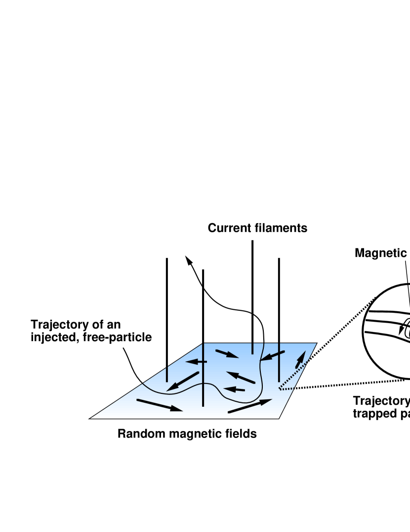
Figure 2: Schematics of the trajectories of a test free particle with energy exceeding a threshold potential energy $|qA|_{\rm th}$, and a gyrating, bound particle with energy below the local potential $|qA(x,y)|$ (light solid curves with arrow). In the energy hierarchy, the transition from the bound state to the free state can be compared to the particle injection for the present DSA, which requires the unbound particles to suffer successive small deflections by the random magnetic fields. For an explanation, see the text. [See the electronic edition of the Journal for a color version of this figure.]

Summarizing the above discussions, there seem to exist two distinct energy regimes for the test particles confined in the system comprising numerous magnetized filaments: the higher energy regime of $E\gg|qA|$, in which the particles are free from the local magnetic traps, and the lower energy regime of $E\ll|qA|$, in which the particles are bound to the local fields, as compared to a low-$\beta$ state. The hierarchy is illustrated in Figure 2, indicating the characteristic trajectories of those particles. When shock propagation is allowed, as seen in actual AGN jets, the shock accelerator can energize the particles in each energy level. At the moment, we are particularly concerned with EHE particle production by a feasible scenario according to which energetic free particles, unbound to small-scale structure of the magnetized filaments, are further energized by the shock. In this aspect, the particle escape from magnetically bound states, due to another energization mechanism, can be regarded as the injection of preaccelerated particles into the concerned diffusive shock accelerator. If the preaccelerator, as well, is of DSA, relying on the gyromotion of bound particles (Drury, 1983; Biermann & Strittmatter, 1987; Zank et al., 2004), the preaccelerator also calls for the injection (in a conventional sense) in a far lower energy level, owing to, e.g., the Maxwellian tail, or the energization of particles up to the energies where the pre-DSA turns on (for a review, see Berezinskiĭ et al., 1990). The energy required for this injection, the so-called injection energy, could be determined by, e.g., the competition with collisional resistance. In order to distinguish from this commonly used definition of “injection,” we refer to the corresponding one, owing to the particle escape from the magnetic traps, as the “transition injection,” in analogy to the bound-free transition in atomic excitation. The energy required to accomplish of the transition injection is formally denoted as $E_{\rm inj}\sim|qA|_{\rm th}$, where $|qA|_{\rm th}$ represents a threshold potential energy. That is, the particles with $q$ and the energy exceeding $E_{\rm inj}$ are considered to spaciously meander to experience successive small deflection by the fields of many filaments (Fig. 2), such that the present theory is adequate for describing the particle diffusion. This scattering property can be compared to that for the conventional QLT in low-$\beta$ regimes: an unperturbed (zeroth order) guiding center trajectory of gyrating particles bound to a mean magnetic field must be a good approximation for many coherence lengths of particle scatterer.

If both the injection and transition injection work, the multistep DSA can be realized. In the stage of $E\ll|qA({\bf r})|$, many acceleration scenarios that have been proposed thus far (DSA: e.g., Drury 1983; Biermann & Strittmatter 1987; shock drift acceleration: e.g., Webb et al. 1983; some versions of the combined theories: e.g., Jokipii 1987; Ostrowski 1988; for a review, see, e.g., Jones & Ellison 1991) can be candidates for the mechanism of the preacceleration up to the energy range of $E\sim|qA({\bf r})|$, although before achieving this energy level, the acceleration, especially for electrons, might be, in some cases, knocked down by the energy loss, such as synchrotron cooling, collision with photons, and so on. The relevant issues for individual specific situations are somewhat beyond the scope of this paper (observability is discussed in § 4). Here we just briefly mention that in the termination regions of large-scale jets where the bulk kinetic energy is significantly converted into the magnetic and particle energies, a conventional DSA mechanism involving large-scale MHD turbulence might work up to EHE ranges (Honda & Honda [2004b] for an updated scenario of oblique DSA of protons).

3.2 Timescale of the Diffusive Shock Acceleration

In the following, we focus on the DSA of energetic free particles after the transition injection. Let us consider a typical case of $\phi_{\rm I}=\phi_{\rm II}=0^{\circ}$ in equation (35), reflecting a reasonable situation that a shock wave propagates along the jet comprising linear filaments. Since the vectors of the random magnetic fields are on the plane transverse to the current filaments, this plane is perpendicular to the shock-normal direction. That is, the shock across the perpendicular magnetic fields is considered. In this case, no irregularity of magnetic surfaces in the shock-normal direction exists, because of $k_{\parallel}=0$. However, this does not mean that the particle flux diffusively across the shock surface is in free-streaming; note that the particles crossing the local fields with nonsmall pitch angles suffer the orthogonal deflection.

Anyhow, the injected particles are off-resonantly scattered by the filamentary turbulence, to diffuse, migrating back and forth many times between the upstream and downstream regions of the shock. As a consequence, a small fraction of them can be stochastically accelerated to very high energy. This scenario is feasible, as long as the filamentary structure can exist around the discontinuity, as seen in a kinetic simulation for shock propagation (Nishikawa et al., 2003) and an actual filamentary jet (Owen et al., 1989). The timescale of this type of DSA is of the order of the cycle time for one back-and-forth divided by the energy gain per encounter with the shock (Gaisser, 1990). Here the cycle time is related to the mean residence time of particles (in regions I and II), which is determined by the diffusive particle flux across the shock, dependent on $\kappa_{{\rm n},\zeta}$ (eq. [35]). For the moment, the shock speed is assumed to be nonrelativistic. Actually, this approximation is reasonable, since the discrete knots (for FR I) and hot spots (for FR II), which are associated with shocks (e.g., Biretta et al., 1983; Carilli & Barthel, 1996), preferentially move at a nonrelativistic speed, slower than the speed of the relativistic jets (e.g., Meisenheimer et al., 1989; Biretta et al., 1995). When taking the first-order Fermi mechanism into consideration for calculation of the energy gain, the mean acceleration time can be expressed as (Lagage & Cesarsky, 1983a, b; Drury, 1983)

$$t_{\rm acc}\simeq{3\over{U_{\rm I}-U_{\rm II}}}\left({\kappa_{\rm n,I}\over U_{\rm I}}+{\kappa_{\rm n,II}\over U_{\rm II}}\right),$$ (37)

where $U_{\rm I}$ and $U_{\rm II}$ are the flow speed of the upstream and downstream regions in the shock rest frame, respectively. The present case of $\phi_{\zeta}=0$ (in eq. [35]) provides $\kappa_{{\rm n},\zeta}=\kappa_{\parallel,\zeta}$, where $\kappa_{\parallel,\zeta}$ is given in equation (30). Here note the relation of $B_{\rm I}=B_{\rm II}$, derived from the condition that the current density, ${\bf J}_{\zeta}\sim\nabla\times{\bf B}_{\zeta}$, must be continuous across the shock front. When assuming $\alpha_{\rm I}=\alpha_{\rm II}$ and $\beta_{\rm I}=\beta_{\rm II}$, we arrive at the result

$$t_{a,{\rm acc}}\simeq{{3\sqrt{6}\pi\alpha r\left(r+1\right)}\over{8\left(\alpha-1\right)\left(\beta_{a}+1\right)\left(\beta_{a}+2\right)\left(r-1\right)}}{cE_{a}^{2}\over{q_{a}^{2}B^{2}RU^{2}}},$$ (38)

where the definitions of $\alpha\equiv\alpha_{\zeta}$, $\beta_{a}\equiv\beta_{\zeta}$, $B\equiv B_{\zeta}$, and $U\equiv U_{\rm I}=rU_{\rm II}$ have been introduced. Equation (38) is valid for arbitrary species of particles “$a$” having energy $E_{a}$, spectral index $\beta_{a}$, and charge $q_{a}$. Note that for the plausible ranges of the values of $\alpha$, $\beta_{a}$, and $r$, the value of equation (38) does not significantly change. The $\phi_{\zeta}$ dependence is also small, because of ${\tilde{\kappa}}\approx 1$, reflecting three-dimensional rms deflection of unbound particles (§ 3.1 and Fig. 2). In the scaling laws shown below, for convenience we use the typical values of $\alpha=2$ (Montgomery & Liu, 1979) and $r=4$ (for the strong shock limit), although we indicate, in equation (43), the parameter dependence of the numerical factor.

3.3 The Highest Energy of an Accelerated Ion

In equation (38) for ions ($a=$”i”), we set $q_{\rm i}=Z|e|$ (see footnote 1) and $\beta_{\rm i}=3$ (e.g., Stecker & Salamon, 1999; de Marco et al., 2003). By balancing equation (38) with the timescale of the most severe energy loss process, we derive the maximum possible energy defined as $E_{\rm i,max}\equiv E_{\rm i}$. In the environment of astrophysical filaments including extragalactic jets, the phenomenological time balance equation can be expressed as

$$t_{{\rm i},{\rm acc}}={\rm min}\left(t_{\rm sh},t_{\rm i,syn},t_{\rm n\gamma},t_{\rm nn^{\prime}}\right),$$ (39)

where $t_{\rm sh}$, $t_{\rm i,syn}$, $t_{\rm n\gamma}$, and $t_{\rm nn^{\prime}}$ stand for the timescales of the shock propagation (§ 3.3.1; eq. [40]), the synchrotron loss for ions (§ 3.3.2; eq. [44]), the photodissociation of the nucleus (§ 3.3.3; e.g., eq. [47]), and the collision of nucleus “${\rm n}$” with target nucleus “${\rm n}^{\prime}$” (§ 3.3.4; e.g., eq. [50]), respectively. In addition, the energy constraint ascribed to the spatial scale, i.e., the quench caused by the particle escape, should also be taken into account (§ 3.3.5). The individual cases are investigated below.

3.3.1 The Case Limited by the Shock Propagation Time

In the actual circumstances of astrophysical jets, the propagation time of a shock through the jet, $t_{\rm sh}$, restricts the maximum possible energy of accelerated particles. The shock propagation time may be interpreted as the age of knots or hot spots (Honda & Honda, 2004b), which can be crudely estimated as $\sim L/U_{\rm prop}$, where $L$ represents a distance from the central engine to the knot or hot spot being considered and $U_{\rm prop}$ an average speed of their proper motion. When assuming $U\sim U_{\rm prop}$, we get the scaling

$$t_{\rm sh}\sim 1\times 10^{11}{L\over{1~{}{\rm kpc}}}{{0.1c}\over{U}}~{}~{}{\rm s}.$$ (40)

For the case in which the shock is currently alive as is observed in AGN jets, $t_{\rm sh}$ cannot be compared to the “lifetime” of the accelerator that is considered in SNR shocks (e.g., Gaisser, 1990).

It is mentioned that in AGN jets, the timescale of adiabatic expansion loss might be estimated as $t_{\rm ad}\approx 3L/\left(2\Gamma U_{r}\right)$, where $\Gamma$ and $U_{r}$ represent the Lorentz factor of jet bulk flows and the speed of radial expansion, respectively (Mücke et al., 2003). The fact that the jets are collimating well with an opening angle of $\phi_{\rm oa}\lesssim 10\arcdeg$ means $U_{\rm prop}/U_{r}\gtrsim O(10)$; thereby, $t_{\rm sh}\lesssim t_{\rm ad}$ for $\Gamma\lesssim{\cal O}(10)$. Thus, it is sufficient to pay attention to the limit due solely to the shock propagation time. These circumstances are also in contrast with those in the SNRs, where the flows are radially expanding without collimation, and the shock propagation time (or lifetime) just reflects the timescale of adiabatic expansion loss (e.g., Longair, 1992).

In equation (39), let us first consider the case of $t_{\rm i,acc}=t_{\rm sh}$. By equating (38) with (40), we obtain the following expression for the maximum possible energy of an accelerated ion:

$$E_{{\rm i},{\rm max}}\sim 70~{}Z{B\over{1~{}{\rm mG}}}\left({L\over{1~{}{\rm kpc}}}\right)^{1/2}\left({R\over{100~{}{\rm pc}}}\right)^{1/2}\left({U\over{0.1c}}\right)^{1/2}~{}~{}{\rm EeV}.$$ (41)

Note the ratio of $L/R\sim 360/(\pi\phi_{\rm oa}\sin\phi_{\rm va})\sim 10-100$ for the narrow opening angle of AGN jets of $\phi_{\rm oa}\sim 1\arcdeg-10\arcdeg$ and not-so-small viewing angle $\phi_{\rm va}$ (e.g., for the M87 jet, $L\simeq 23R-33R$ for $\phi_{\rm oa}\simeq 6\fdg 9$ [Reid et al. 1989] and $\phi_{\rm va}=42\fdg 5\pm 4\fdg 5$ [Biretta et al. 1995] or $30\arcdeg-35\arcdeg$ [Bicknell & Begelman 1996]). Equation (41) (and eq. [52] shown below) corresponds to the modified version of the simple scaling originally proposed by Hillas (1984).

Concerning the abundance of high-$Z$ elements and their acceleration to EHE regimes, the following points 1–4 may be worth noting:

1. Radial metallicity gradients are expected to be enhanced in elliptical galaxies (e.g., Kobayashi, 2004). Along with this, a significant increase of heavy elements has been discovered in the central region of the nearby giant elliptical galaxy M87 (Gastaldello & Molendi, 2002), which contains a confirmed jet.

2. A variety of heavy ions including iron have been detected in a microquasar jet (SS 433; Kotani et al., 1996).

3. The Haverah Park data favor proton primaries below an energy of $\sim 50~{}{\rm EeV}$, whereas they appear to favor a heavier composition above it (Ave et al., 2000).

4. The recent Fly’s Eye data of $\sim 320~{}{\rm EeV}$ are compatible with the assumption of a hadron primary between proton and iron nuclei (Risse et al., 2004).

With reference to this observational evidence, we take the possibility of acceleration of (or deceleration by) heavy particles into consideration and indicate the charge ($Z$) and/or atomic number ($A$) dependence of the maximum possible energies and loss timescales.

3.3.2 The Case Limited by the Synchrotron Cooling Loss

The particles deflected by the random magnetic fields tend to emit unpolarized synchrotron photons, which can be a dominant cooling process. For relativistic ions, the timescale can be written as $t_{\rm i,syn}\simeq 36\pi^{2}(A/Z)^{4}[m_{\rm p}^{4}c^{7}/(e^{4}B^{2}E_{\rm i})]$, where $m_{\rm p}$ denotes the proton rest mass (Gaisser, 1990). In this expression, the energy of an accelerated ion, $E_{\rm i}$, can be evaluated by equating $t_{\rm i,acc}$ with $t_{\rm i,syn}$. That is, we have

$${E_{\rm i}\over{Am_{\rm p}c^{2}}}=\xi(\alpha,\beta_{\rm i},r)\left[{A\over Z^{2}}{{m_{\rm p}}\over{m_{\rm e}}}{R\over r_{0}}\left({U\over c}\right)^{2}\right]^{1/3}.$$ (42)

Here the dimensionless factor $\xi$ is given by

$$\xi(\alpha,\beta,r)=\left[{{4\sqrt{6}\left(\alpha-1\right)\left(\beta+1\right)\left(\beta+2\right)\left(r-1\right)}\over{\alpha r\left(r+1\right)}}\right]^{1/3},$$ (43)

and $r_{0}=e^{2}/(4\pi m_{\rm e}c^{2})$ stands for the classical radius of the electron, where $m_{\rm e}$ is the electron rest mass. Substituting equation (42) into the expression of $t_{\rm i,syn}$, the cooling timescale can be expressed as a function of the physical parameters of the target object. As a result, we find

$$t_{\rm i,syn}\sim 3\times 10^{15}{1\over Z^{2/3}}\left({A\over{2Z}}\right)^{8/3}\left({{1~{}{\rm mG}}\over B}\right)^{2}\left({{100~{}{\rm pc}}\over{R}}\right)^{1/3}\left({{0.1c}\over{U}}\right)^{2/3}~{}~{}{\rm s}.$$ (44)

Practically, this expression can be used in equation (39) for making a direct comparison with the other loss timescales. For example, in the FR sources with $B\lesssim 1~{}{\rm mG}$ (Owen et al., 1989; Meisenheimer et al., 1989, 1996; Rachen & Biermann, 1993), we have $t_{\rm i,syn}\gg t_{\rm sh}$, so that the synchrotron cooling loss is ineffective. It should, however, be noted that in blazars with $B\gtrsim 0.1~{}{\rm G}$ (Kataoka et al., 1999; Mücke & Protheroe, 2001; Aharonian, 2002), equation (44) becomes, in some cases, comparable to equation (40).

When the equality of $t_{\rm i,acc}=t_{\rm i,syn}$ is fulfilled in equation (39), equation (42) just provides the maximum possible energy of the accelerated ion, which scales as

$$E_{\rm i,max}\sim 2A^{2/3}\left({A\over{2Z}}\right)^{2/3}\left({R\over{100~{}{\rm pc}}}\right)^{1/3}\left({U\over{0.1c}}\right)^{2/3}~{}~{}{\rm ZeV}.$$ (45)

The important point is that $t_{\rm i,acc}$ and $t_{\rm i,syn}$ are both proportional to $B^{-2}$, so that the $B$ dependence of $E_{\rm i,max}$ is canceled out. This property also appears in the case of electron acceleration attenuated by the synchrotron cooling (§ 3.4.1). In equation (45), it appears that for heavier ions, $E_{\rm i,max}$ takes a larger value. In the actual situation, however, the extremely energetic ions possess a long mfp, and therefore, acceleration may be quenched by the particle escape, as discussed in § 3.3.5.

3.3.3 The Case Limited by the Collision with Photons

Here we focus on the proton-photon collision that engenders a pion-producing cascade. The characteristic time of the collision depends on the target photon spectrum $n(\epsilon_{\rm ph})$ in the acceleration site, where $n(\epsilon_{\rm ph})$ is the number density of photons per unit energy interval for photon energy $\epsilon_{\rm ph}$. For $n(\epsilon_{\rm ph})\propto\epsilon_{\rm ph}^{-2}$ (e.g., Bezler et al., 1984), typical for the FR sources (Rachen & Biermann, 1993), the timescale can be expressed as $t_{{\rm p}\gamma}\sim[u_{\rm m}/(\chi u_{\rm ph})]t_{\rm p,syn}$, where $\chi\sim 200$ for the average cross section of $\sigma_{\gamma{\rm p}}\sim 900~{}{\rm\mu barns}$ (Biermann & Strittmatter, 1987), $u_{\rm ph}$ denotes the average energy density of target photons, and $t_{\rm p,syn}=t_{\rm i,syn}|_{A=Z=1}$ (the subscript “p” indicates proton). Thus, the expression of $t_{{\rm p}\gamma}$ includes $E_{\rm p}$, i.e., the energy of the accelerated proton. This can be evaluated by equating $t_{\rm p,acc}$ with $t_{{\rm p}\gamma}$, to have the form of

$${E_{\rm p}\over{m_{\rm p}c^{2}}}={{\xi(\alpha,\beta_{\rm i},r)}\over{\left(\chi\eta_{u}\right)^{1/3}}}\left[{{m_{\rm p}}\over{m_{\rm e}}}{R\over r_{0}}\left({U\over c}\right)^{2}\right]^{1/3},$$ (46)

where the definition $\eta_{u}\equiv u_{\rm ph}/u_{\rm m}$ has been introduced. Substituting equation (46) into the expression of $t_{{\rm p}\gamma}$, we obtain the following scaling of the photomeson cooling time:

$$t_{{\rm p}\gamma}\sim 6\times 10^{15}\left({200\over\chi}\right)^{2/3}\eta_{u}^{1/3}{{10^{-10}~{}{\rm erg}~{}{\rm cm}^{-3}}\over{u_{\rm ph}}}\left({{100~{}{\rm pc}}\over{R}}\right)^{1/3}\left({{0.1c}\over{U}}\right)^{2/3}~{}~{}{\rm s}.$$ (47)

Note that for $\eta_{u}=\chi^{-1}\sim 5\times 10^{-3}$, we have $t_{{\rm p}\gamma}=t_{\rm p,syn}$.

If the equality of $t_{\rm p,acc}=t_{{\rm p}\gamma}$ is satisfied in equation (39), then equation (46) gives the maximum possible energy, which scales as

$$E_{\rm p,max}\sim 200\left({200\over\chi}\right)^{1/3}\left(1\over\eta_{u}\right)^{1/3}\left({R\over{100~{}{\rm pc}}}\right)^{1/3}\left({U\over{0.1c}}\right)^{2/3}~{}~{}{\rm EeV}.$$ (48)

For $\eta_{u}=\chi^{-1}$, equation (48) is identical with equation (45) for $A=Z=1$.

3.3.4 The Case Limited by the Collision with Particles

The nucleus-nucleus collisions involving spallation reactions can also be a competitive process in high-density regions. For proton-proton collision, the timescale can be simply evaluated by $t_{\rm pp^{\prime}}=(n_{\rm p^{\prime}}\sigma_{\rm pp^{\prime}}c)^{-1}$, where $n_{\rm p^{\prime}}$ is the number density of target protons, and $\sigma_{\rm pp^{\prime}}\approx 40~{}{\rm mbarns}$ denotes the cross section in high-energy regimes. The timescale can be rewritten as

$$t_{\rm pp^{\prime}}\simeq 8.3\times 10^{14}{{1~{}{\rm cm}^{-3}}\over{n_{\rm p^{\prime}}}}~{}~{}{\rm s}.$$ (49)

It is found that for tenuous jets with $n_{\rm p^{\prime}}\ll 1~{}{\rm cm}^{-3}$, the value of equation (49) is larger than the conceivable value of equation (40); that is, the collisional loss is ineffective.

For the collision of an accelerated proton with a nonproton nucleus, the timescale can be evaluated by the analogous notation, $t_{\rm p{\rm N}^{\prime}}=(n_{A^{\prime}}\sigma_{{\rm p}A^{\prime}}c)^{-1}$, where $n_{A^{\prime}}$ is the fractional number density of the target nuclei having atomic number $A^{\prime}>1$. Here we use an empirical scaling of the cross section, $\sigma_{{\rm p}A^{\prime}}\approx\pi r_{0}^{2}A^{\prime 2/3}$, where $r_{0}\simeq 1.4\times 10^{-13}~{}{\rm cm}$, although the value of $r_{0}$ may be an overestimate for very high energy collisions (e.g., Burbidge, 1956). Combining $t_{\rm p{\rm N}^{\prime}}$ with $t_{\rm pp^{\prime}}$, in general the timescale for collision of a proton with a nucleus of an arbitrary composition can be expressed as

$$t_{\rm pn^{\prime}}\simeq 5.4\times 10^{14}{1\over{0.65n_{\rm p^{\prime}}+\sum_{A^{\prime}>1}n_{A^{\prime}}A^{\prime 2/3}}}~{}~{}{\rm s},$$ (50)

where $n_{\rm p^{\prime}}$ and $n_{A^{\prime}}$ are both in units of ${\rm cm}^{-3}$.

In equation (39), we consider the case of $t_{\rm p,acc}=t_{\rm pn^{\prime}}$. By equating (38) with (50), we obtain the following expression for the maximum possible energy of an accelerated proton:

$$E_{\rm p,max}\sim 200\left({{100~{}{\rm cm}^{-3}}\over{n_{\rm p^{\prime}}+1.5\sum_{A^{\prime}>1}n_{\rm A^{\prime}}A^{\prime 2/3}}}\right)^{1/2}{B\over{1~{}{\rm mG}}}\left({R\over{100~{}{\rm pc}}}\right)^{1/2}{U\over{0.1c}}~{}~{}{\rm EeV}.$$ (51)

As for the collision of an arbitrary accelerated nucleus with a target nucleus, we can analogously estimate $t_{\rm nn^{\prime}}$ and $E_{\rm i,max}$. In particular, the heavier nucleus–proton collision is more important, since its timescale $t_{\rm np^{\prime}}$ is of the order of $t_{\rm pp^{\prime}}/A^{2/3}$: for larger $A$ and $n_{\rm p^{\prime}}$, it can be comparable to the other loss timescales. For example, the parameters of $A=56$ (iron) and $n_{\rm p^{\prime}}\sim 100~{}{\rm cm}^{-3}$ lead to $t_{\rm np^{\prime}}\sim 4\times 10^{11}~{}{\rm s}$. For the case of $t_{\rm i,acc}=t_{\rm np^{\prime}}$ in equation (39), we have the scaling of $E_{\rm i,max}\sim 0.6Z^{2/3}(2Z/A)^{1/3}E_{\rm p,max}$, where $E_{\rm p,max}$ is of equation (51) for $n_{\rm p^{\prime}}\gg\sum_{A^{\prime}>1}n_{A^{\prime}}A^{\prime 2/3}$.

3.3.5 Quenching by Particle Escape

The particle escape also limits its acceleration; that is, the spatioscale of the system brings on another energy constraint. Relating to this point, in § 2.4 we found the relation of ${\tilde{\kappa}}\approx 1$, meaning that the anisotropy of the spatial diffusion coefficient is small. It follows that the radial size of the jet (rather than $L$) affects the particle confinement. Recall here that in the interior of a jet the magnetic field vectors tend to be canceled out, whereas around the envelope the uncanceled, large-scale ordered field can appear (Honda & Honda, 2004a). From the projected view of the jet, on both sides of the envelope the magnetic polarities are reversed.

The spatially decaying properties of such an envelope field in the external tenuous medium or vacuum might influence the transverse diffusion of particles. The key property that should be recalled is that for $r\gg k^{-1}$ distant from a filament, the magnetic field strength is likely to slowly decay, being proportional to $\sim(kr)^{-1}$ (Honda, 2000; Honda & Honda, 2002). It is, therefore, expected that as long as the radial size of the largest filament, i.e., correlation length, is comparable to the radius of the jet (§ 2.3), the long-range field pervades the exterior of the jet, establishing the “magnetotail” with the decay property of $\sim(k_{\rm min}r)^{-1}$ for $r\gg k_{\rm min}^{-1}(\sim R)$. In fact, in a nearby radio galaxy, the central kiloparsec-scale “hole” of the inner radio lobe containing a jet is filled with an ordered, not-so-weak (rather strong) magnetic field of the order of $10-100~{}{\rm\mu G}$ (Owen et al., 1990), whose magnitude is comparable to (or $\sim 10~{}\%$ of) that in the jet (Owen et al., 1989; Heinz & Begelman, 1997). Presumably, the exuding magnetic field plays an additional role in confining the leaky energetic particles with their long mfp of $\lambda_{\perp}(\sim c\psi_{2}/\nu_{22})\sim R$.

In this aspect, let us express an effective confinement radius as $R_{\rm c}={\tilde{\rho}}R$, where ${\tilde{\rho}}\gtrsim 1$, and impose the condition that the accelerator operates for the particles with the transverse mfp of $\lambda_{\perp}\leq R_{\rm c}$. Then the equality gives the maximum possible energy in the form of

$$E_{\rm i,max}\sim 200~{}Z{\tilde{\rho}}^{1/2}{B\over{1~{}{\rm mG}}}{R\over{100~{}{\rm pc}}}~{}~{}{\rm EeV}.$$ (52)

Values of $E_{\rm i,max}$ (and $E_{\rm p,max}$) derived from the time balance equation (39) cannot exceed that of equation (52). It appears that equation (52) can be compared to the energy scaling derived from, in the simplest model, the maximum gyroradius in a uniform magnetic field.

3.4 The Highest Energy of an Accelerated Electron

In a manner simiar to that explained in § 3.3, we find the generic scaling for the achievable highest energy of electrons. In equation (38) for electrons ($a=$”e”), we set $q_{\rm e}=-|e|$ and $\beta_{\rm e}=2$ (e.g., Meisenheimer et al., 1989; Rachen & Biermann, 1993; Wilson & Yang, 2002). By balancing equation (38) with the timescale of a competitive energy loss process, we derive the maximum possible energy defined as $E_{\rm e,max}\equiv E_{\rm e}$. The time balance equation can be written as

$$t_{{\rm e},{\rm acc}}={\rm min}\left(t_{\rm e,syn},t_{\rm ic},t_{\rm br}\right),$$ (53)

where $t_{\rm e,syn}$, $t_{\rm ic}$, and $t_{\rm br}$ stand for the timescales of the synchrotron loss for electrons (§ 3.4.1; eq. [55]), the inverse Compton scattering (§ 3.4.2; eq. [58]), and the bremsstrahlung emission loss (§ 3.4.3; eq. [61]), respectively. For positrons the method is so analogous that we omit the explanation.

3.4.1 The Case Limited by the Synchrotron Cooling Loss

For electrons, the synchrotron cooling is a familiar loss process, and the timescale can be expressed as $t_{\rm e,syn}\simeq 36\pi^{2}m_{\rm e}^{4}c^{7}/(e^{4}B^{2}E_{\rm e})$. In this expression, the energy of an accelerated electron, $E_{\rm e}$, can be evaluated by equating $t_{\rm e,acc}$ with $t_{\rm e,syn}$, to give

$${E_{\rm e}\over{m_{\rm e}c^{2}}}=\xi(\alpha,\beta_{\rm e},r)\left[{R\over r_{0}}\left({U\over c}\right)^{2}\right]^{1/3}.$$ (54)

Substituting equation (54) into the aforementioned expression of $t_{\rm e,syn}$, the cooling timescale can be expressed as a function of the physical parameters of the target object:

$$t_{\rm e,syn}\sim 1\times 10^{6}\left({{1~{}{\rm mG}}\over B}\right)^{2}\left({{100~{}{\rm pc}}\over{R}}\right)^{1/3}\left({{0.1c}\over{U}}\right)^{2/3}~{}~{}{\rm s}.$$ (55)

This can be used in equation (53) for comparison with the other loss timescales.

When the equality of $t_{\rm e,acc}=t_{\rm e,syn}$ is satisfied in equation (53), equation (54) gives the maximum possible energy, which scales as

$$E_{\rm e,max}\sim 50\left({R\over{100~{}{\rm pc}}}\right)^{1/3}\left({U\over{0.1c}}\right)^{2/3}~{}~{}{\rm PeV}.$$ (56)

According to the explanation given in § 3.3.2, equation (56) is independent of $B$ (see also eq. [45]). The striking thing is that for plausible parameters, the value of $E_{\rm e,max}$ is significantly larger than that obtained in the context of the simplistic QLT invoking the Alfvén waves (Biermann & Strittmatter, 1987). This enhancement is, as seen in equation (32), attributed to the smaller value of the diffusion coefficient for electrons, which leads to a shorter acceleration time, i.e., a smaller value of equation (37), and thereby to a higher acceleration efficiency.

3.4.2 The Case Limited by the Inverse Compton Scattering

For the case of $\eta_{u}>1$, the inverse Compton scattering of accelerated electrons with target photons can be a dominant loss process. Actually, the environments of AGN jets often allow the synchrotron self-Compton (SSC) and/or external Compton (EC) processes. The characteristic time of the inverse Comptonization can be estimated as $t_{\rm ic}\sim(t_{\rm e,syn}/\eta_{u})(\sigma_{\rm T}/\sigma_{\rm KN})$, where $\sigma_{\rm T}=8\pi r_{0}^{2}/3$ and $\sigma_{\rm KN}(\epsilon_{\rm ph}E_{\rm e})$ denote the total cross sections in the Thomson limit of $\epsilon_{\rm ph}E_{\rm e}\ll m_{\rm e}^{2}c^{4}$ and the Klein-Nishina regime of $\epsilon_{\rm ph}E_{\rm e}\gtrsim m_{\rm e}^{2}c^{4}$, respectively (e.g., Longair, 1992). The expression of $t_{\rm ic}$ includes $E_{\rm e}$, which is determined by numerically solving the balance equation of $t_{\rm e,acc}=t_{\rm ic}$. Because of $\sigma_{\rm KN}\leq\sigma_{\rm T}$, the value of $E_{\rm e}$ is found to be in the region of

$${E_{\rm e}\over{m_{\rm e}c^{2}}}\geq{{\xi(\alpha,\beta_{\rm e},r)}\over{\eta_{u}^{1/3}}}\left[{R\over r_{0}}\left({U\over c}\right)^{2}\right]^{1/3},$$ (57)

in the whole range of $\epsilon_{\rm ph}$. Note that the equality in equation (57) reflects the Thomson limit of $\sigma_{\rm KN}/\sigma_{\rm T}=1$. Substituting the value of $E_{\rm e}$ into the expression of $t_{\rm ic}$, we can evaluate the scattering time, which takes a value in the range of

$$t_{\rm ic}\geq 5\times 10^{8}\eta_{u}^{1/3}{{10^{-10}~{}{\rm erg}~{}{\rm cm}^{-3}}\over{u_{\rm ph}}}\left({{100~{}{\rm pc}}\over{R}}\right)^{1/3}\left({{0.1c}\over{U}}\right)^{2/3}~{}~{}{\rm s}.$$ (58)

For a given parameter $\eta_{u}$, the larger value of $u_{\rm ph}$ depresses the lower bound of $t_{\rm ic}$, though the Klein-Nishina effects prolong the timescale. It should be noted that the evaluation of $t_{\rm ic}$ along equation (58) is, in equation (53), meaningful only for $\eta_{u}\geq 1$; that is, the relation of $\eta_{u}<1$ ensures $t_{\rm ic}>t_{\rm e,syn}$.

For the case of $t_{\rm e,acc}=t_{\rm ic}$ in equation (53), $E_{\rm e}$, conforming to equation (57), gives the maximum possible energy, which takes the value of

$$E_{\rm e,max}\geq 50\left({1\over{\eta_{u}}}\right)^{1/3}\left({R\over{100~{}{\rm pc}}}\right)^{1/3}\left({U\over{0.1c}}\right)^{2/3}~{}~{}{\rm PeV}$$ (59)

for $\eta_{u}\geq 1$. Again, note that the Thomson limit sets the lower bound of $E_{\rm e,max}$. It is found that the Klein-Nishina effects enhance the value of $E_{\rm e,max}$ in the regime of $\epsilon_{\rm ph}\gtrsim m_{\rm e}^{2}c^{4}/E_{\rm e,max}$. Note here that $E_{\rm e,max}$ cannot unlimitedly increase in actual circumstances but tends to be limited by the synchrotron cooling. Combining equation (56) with equation (59), therefore, we can express the allowed domain of the variables as follows:

$$1\geq{E_{\rm e,max}\over{50~{}{\rm PeV}}}\left({{100~{}{\rm pc}}\over R}\right)^{1/3}\left({{0.1c}\over U}\right)^{2/3}\geq{1\over{\eta_{u}^{1/3}}}.$$ (60)

Note that the upper bound reflects the synchrotron limit. In the critical case of $\eta_{u}=1$ reflecting the energy equipartition, the generic equation (60) degenerates into equation (56).

3.4.3 The Bremsstrahlung Loss

The bremsstrahlung emission of electrons in the Coulomb field of nuclei whose charge is incompletely screened also affects the acceleration. The timescale can be evaluated by the notation $t_{\rm br}=(n_{Z^{\prime}}\sigma_{{\rm rad,e}Z^{\prime}}c)^{-1}$, where $n_{Z^{\prime}}$ is the fractional number density of the target nuclei having charge number $Z^{\prime}$ and $\sigma_{{\rm rad,e}Z^{\prime}}$ describes the radiation cross section (e.g., Heitler, 1954). When the screening effects are small, for interaction with a heavy composite we have

$$t_{\rm br}\simeq 1.4\times 10^{16}\left\{\left[22+{\rm ln}\left(E_{\rm e}/1~{}{\rm PeV}\right)\right]\sum_{Z^{\prime}}n_{Z^{\prime}}Z^{\prime 2}\right\}^{-1}~{}~{}{\rm s},$$ (61)

where $n_{Z^{\prime}}$ is in units of ${\rm cm}^{-3}$.

In the peculiar environments of high density, enhanced metallicity, and lower magnetic and photon energy densities, equation (61) may be comparable with equation (55) or (58). In ordinary AGN jets, however, the corresponding physical parameters seem to be marginal. Note also that the bremsstrahlung timescale for ion-ion interactions is larger, by the order of $(A^{2}/Z^{4})(m_{\rm p}/m_{e})^{2}\sim 10^{7}/Z^{2}$, than the value of equation (61), and found to largely exceed the value of equation (40), namely, the age of the accelerator. That is why the ion bremsstrahlung has been excluded in equation (39).

4 DISCUSSION AND SUMMARY

The feasibility of the present model could be verified by the measurement of energetic photons emanating from a source, typically, bright knots in nearby AGN jets. In any case, the electrons with energy $E_{\rm e,max}$, given in equation (60), emit the most energetic synchrotron photons, whose frequency may be estimated as $\nu^{\ast}\sim(E_{\rm e,max}/m_{\rm e}c^{2})^{2}(eB/m_{\rm e}c)$, where the mean field strength ${\bar{B}}$ has been compared to the rms strength $B$. For $E_{\rm e,max}\sim 10~{}{\rm PeV}$ as an example, the frequencies of $\nu^{\ast}\gtrsim 10^{22}~{}{\rm Hz}$ are found to be achieved for $B\gtrsim 10~{}{\rm\mu G}$. In the gamma-ray bands, however, the energy flux of photons from the synchrotron originator is predicted to be often overcome by that produced by the inverse Comptonization of target photons. In this case, as far as the condition of $\epsilon_{\rm ph}E_{\rm e,max}\gg(m_{\rm e}c^{2})^{2}$ is satisfied, the boosted photon energy is given by $\epsilon_{\rm ph}^{\prime}\sim E_{\rm e,max}$, independent of the target photon energy $\epsilon_{\rm ph}$, thereby irrespective of SSC or ECs. This is in contrast to another case of $\epsilon_{\rm ph}E_{\rm e,max}\ll(m_{\rm e}c^{2})^{2}$, in which one has $\epsilon_{\rm ph}^{\prime}\sim\epsilon_{\rm ph}(E_{\rm e,max}/m_{\rm e}c^{2})^{2}$ dependent on $\epsilon_{\rm ph}$. Apparently, for the extremely high energy ranges of $E_{\rm e,max}$ achieved in the present scheme, the former condition is more likely satisfied for a wide range of $\epsilon_{\rm ph}$. Therefore, in the circumstances that the source is nearby such that collision with the cosmic infrared background, involving photon-photon pair creation, is insignificant, $\epsilon_{\rm ph}^{\prime}$ ($\sim E_{\rm e,max}$) just gives the theoretical maximum of gamma-ray energy, although the Klein-Nishina effects also take part in lowering the flux level. This means, in turn, that a comparison of the $\epsilon_{\rm ph}^{\prime}$ value (multiplied by an appropriate Doppler factor) with the observed highest energy of the Compton emissions might constitute a method to verify the present DSA for electrons.

The case for this method is certainly solidified when the operation of the transition injection (§ 3.1) is confirmed. Making use of the inherent property that the synchrotron photons emitted by electrons having an energy above $|eA({\bf r})|$ reduce their polarization, the energy hierarchy can be revealed by the polarization measurements, particularly, with wide frequency ranges and high spatioresolution. According to the reasoning that the critical frequency above which the measured polarization decreases, $\nu_{\rm c}({\bf r})$, ought to be of the order of $\sim[|eA({\bf r})|/m_{\rm e}c^{2}]^{2}[|e{\bf B}({\bf r})|/m_{\rm e}c]$, the related coherence length can be estimated as $k_{\rm c}^{-1}\sim c\{\nu_{\rm c}({\bf r})[m_{\rm e}c/|e{\bf B}({\bf r})|]^{3}\}^{1/2}$. Note that when the locally defined gyroradius reaches this critical scale, the bound electrons are released. In actual circumstances, $\nu_{\rm c}$ and the polarization for a fixed frequency band are, if anything, likely to increase near the jet surface, where the large-scale coherency could appear (§ 3.3.5). This may be responsible for the results of the polarization measurement of a nearby filamentary jet, which indicate a similar transverse dependence (Capetti et al., 1997). In the sense of $E_{\rm e,max}/E_{\rm inj}|_{q=-|e|}\ll E_{\rm i,max}/E_{\rm inj}|_{q=Z|e|}$, the transition injection condition for electrons is more restrictive than that for ions. Thus, observational evidence of the present DSA scenario for energetic electrons will, if it is obtained, strongly suggest that the same scenario operates for ion acceleration, providing its finite abundance.

To summarize, we have accomplished the modeling of the diffusive shock accelerator accompanied by the quasi-static, magnetized filamentary turbulence that could be self-organized via the current filamentation instability. The new theory of particle diffusion relies on the following conditions analogous to those for the conventional QLT: (1) the test particles must not be strongly deflected by a fine filament but suffer the cumulative small deflection by many filaments, and (2) the transverse filament size, i.e., the coherence length of the scatterer, is limited by the system size transverse to the filaments; whereas, more importantly, it is dependent on neither the gyration, the resonant scattering, nor the explicit limit of the weak turbulence. We have derived the diffusion coefficient from the quasi-linear type equation and installed it in a DSA model that involves particle injection associated with the bound-free transition in the fluctuating vector potential. By systematically taking the conceivable energy restrictions into account, some generic scalings of the maximum energy of particles have been presented. The results indicate that the shock in kiloparsec-scale jets could accelerate a proton and heavy nucleus to $10-100~{}{\rm EeV}$ and ${\rm ZeV}$ ranges, respectively. In particular, for high-$Z$ particles, and electrons as well, the acceleration efficiency is significantly higher than that derived from a simplistic QLT-based DSA, as is deduced from equation (32). Consequently, the powerful electron acceleration to ${\rm PeV}$ ranges becomes possible for the plausible parameters.

We expect that the present theory can be, mutatis mutandis, applied for solving the problem of particle transport and acceleration in GRBs (Nishikawa et al., 2003; Silva et al., 2003). The topic is of a cross-disciplinary field closely relevant to astrophysics, high-energy physics, and plasma physics involving fusion science; particularly, the magnetoelectrodynamics of filamentary turbulence is subject to the complexity of “flowing plasma.” In perspective, further theoretical details might be resolved, in part, by a fully kinetic approach allowing multiple dimensions, which goes far beyond the MHD context.

Appendix A CALCULATION OF THE INTEGRAL COMPONENTS $I_{12}$, $I_{21}$, AND $I_{22}$

For instruction, we write down the derivation of equations (24) and (25) for the collisionless scattering of injected test particles by magnetized current filaments having the configuration illustrated in Figure 1. Making use of equation (10), $I_{ij}$ for $ij\neq 11$ (eq. [12]) can be explicitly written as

$$I_{12}=-i{q^{2}\over c^{2}}\int{\rm d}^{2}{\bf k}{\rm d}\omega|A|_{{\bf k},\omega}^{2}\left({\bf k}\cdot{\bf v}\right){\partial\over{\partial p_{\parallel}}}\left\{\left[\omega-\left({\bf k}\cdot{\bf v}\right)\right]^{-1}v_{\parallel}\left({\bf k}\cdot{\partial\over{\partial{\bf p}_{\perp}}}\right)\left<f_{\bf p}\right>\right\},$$ (A1)

$$I_{21}=-i{q^{2}\over c^{2}}\int{\rm d}^{2}{\bf k}{\rm d}\omega|A|_{{\bf k},\omega}^{2}v_{\parallel}\left({\bf k}\cdot{\partial\over{\partial{\bf p}_{\perp}}}\right)\left\{\left[\omega-\left({\bf k}\cdot{\bf v}\right)\right]^{-1}\left({\bf k}\cdot{\bf v}\right){\partial\over{\partial p_{\parallel}}}\left<f_{\bf p}\right>\right\},$$ (A2)

$$I_{22}=i{q^{2}\over c^{2}}\int{\rm d}^{2}{\bf k}{\rm d}\omega|A|_{{\bf k},\omega}^{2}v_{\parallel}\left({\bf k}\cdot{\partial\over{\partial{\bf p}_{\perp}}}\right)\left\{\left[\omega-\left({\bf k}\cdot{\bf v}\right)\right]^{-1}v_{\parallel}\left({\bf k}\cdot{\partial\over{\partial{\bf p}_{\perp}}}\right)\left<f_{\bf p}\right>\right\},$$ (A3)

where we have used a standard correlation function (eq. [13]) reflecting random magnetic fluctuations on the transverse plane to the linear current filaments (see Fig. 1). Recalling the causality principle and noticing that the real part does not contribute to the integration, we get

$$I_{12}=-{{\pi q^{2}}\over c^{2}}\int{\rm d}^{2}{\bf k}{\rm d}{\omega}|A|_{{\bf k},\omega}^{2}\left({\bf k}\cdot{\bf v}\right){\partial\over{\partial p_{\parallel}}}\left\{\delta\left[\omega-\left({\bf k}\cdot{\bf v}\right)\right]v_{\parallel}\left({\bf k}\cdot{\partial\over{\partial{\bf p}_{\perp}}}\right)\left<f_{\bf p}\right>\right\},$$ (A4)

$$I_{21}=-{{\pi q^{2}}\over c^{2}}\int{\rm d}^{2}{\bf k}{\rm d}{\omega}|A|_{{\bf k},\omega}^{2}v_{\parallel}\left({\bf k}\cdot{\partial\over{\partial{\bf p}_{\perp}}}\right)\left\{\delta\left[\omega-\left({\bf k}\cdot{\bf v}\right)\right]\left({\bf k}\cdot{\bf v}\right){\partial\over{\partial p_{\parallel}}}\left<f_{\bf p}\right>\right\},$$ (A5)

$$I_{22}={{\pi q^{2}}\over c^{2}}\int{\rm d}^{2}{\bf k}{\rm d}{\omega}|A|_{{\bf k},\omega}^{2}v_{\parallel}\left({\bf k}\cdot{\partial\over{\partial{\bf p}_{\perp}}}\right)\left\{\delta\left[\omega-\left({\bf k}\cdot{\bf v}\right)\right]v_{\parallel}\left({\bf k}\cdot{\partial\over{\partial{\bf p}_{\perp}}}\right)\left<f_{\bf p}\right>\right\}.$$ (A6)

Again, we use an ad hoc equation (16), valid for a quasi-static mode that retains the narrow spectral peak around $\omega\sim 0$. Assuming that the magnetic turbulence is isotropic on the transverse plane, the angular average of equations (A4)–(A6) is carried out. Taking account of the off-resonant scattering of particles by the quasi-static random fields gives

$$I_{12}\sim-{{16\pi q^{2}}\over c^{2}}v_{\perp}{\partial\over{\partial p_{\parallel}}}\left({v_{\parallel}\over v_{\perp}}\right){\partial\over{\partial p_{\perp}}}\left<f_{\bf p}\right>\int_{k_{\rm min}}^{k_{\rm max}}{{{\rm d}k}\over k}I_{k},$$ (A7)

$$I_{21}\sim-{{16\pi q^{2}}\over c^{2}}v_{\parallel}{\partial^{2}\over{\partial p_{\perp}\partial p_{\parallel}}}\left<f_{\bf p}\right>\int_{k_{\rm min}}^{k_{\rm max}}{{{\rm d}k}\over k}I_{k},$$ (A8)

$$I_{22}\sim{{16\pi q^{2}}\over c^{2}}v_{\parallel}{\partial\over{\partial p_{\perp}}}\left({v_{\parallel}\over v_{\perp}}\right){\partial\over{\partial p_{\perp}}}\left<f_{\bf p}\right>\int_{k_{\rm min}}^{k_{\rm max}}{{{\rm d}k}\over k}I_{k},$$ (A9)

where the ordering and the definition of $I_{k}$ are the same as those denoted in § 2.2. For a given momentum distribution function of $\left<f_{\bf p}\right>\propto|{\bf p}|^{-(\beta+2)}$ for the test particles with an ultrarelativistic energy of $E=|{\bf p}|c=c(p_{\parallel}^{2}+p_{\perp}^{2})^{1/2}$, the partial derivatives can be estimated as

$${\partial\over{\partial p_{\parallel}}}\left({v_{\parallel}\over v_{\perp}}\right){\partial\over{\partial p_{\perp}}}\left<f_{\bf p}\right> \sim \left(\beta+2\right)\left[\left(\beta+3\right)\psi_{1}^{2}-\psi_{2}^{2}\right]{c^{2}\over E^{2}}\left<f_{\bf p}\right>$$ (A10)

$$= {\partial^{2}\over{\partial p_{\parallel}^{2}}}\left<f_{\bf p}\right>,$$

$${\partial^{2}\over{\partial p_{\perp}\partial p_{\parallel}}}\left<f_{\bf p}\right> \sim \left(\beta+2\right)\left(\beta+4\right)\psi_{1}\psi_{2}{c^{2}\over E^{2}}\left<f_{\bf p}\right>$$ (A11)

$$= {\partial\over{\partial p_{\perp}}}\left({v_{\parallel}\over v_{\perp}}\right){\partial\over{\partial p_{\perp}}}\left<f_{\bf p}\right>,$$

where $\psi_{1}\equiv p_{\parallel}/|{\bf p}|$ and $\psi_{2}\equiv p_{\perp}/|{\bf p}|$. Using equations (A10) and (A11), and equation (22) concerning the $k$-space integration for $k_{\rm max}\rightarrow\infty$, one can arrange equations (A7)–(A9) in the form of $I_{ij}\sim\nu_{ij}\left<f_{\bf p}\right>$ to obtain the expressions of equations (24) and (25).

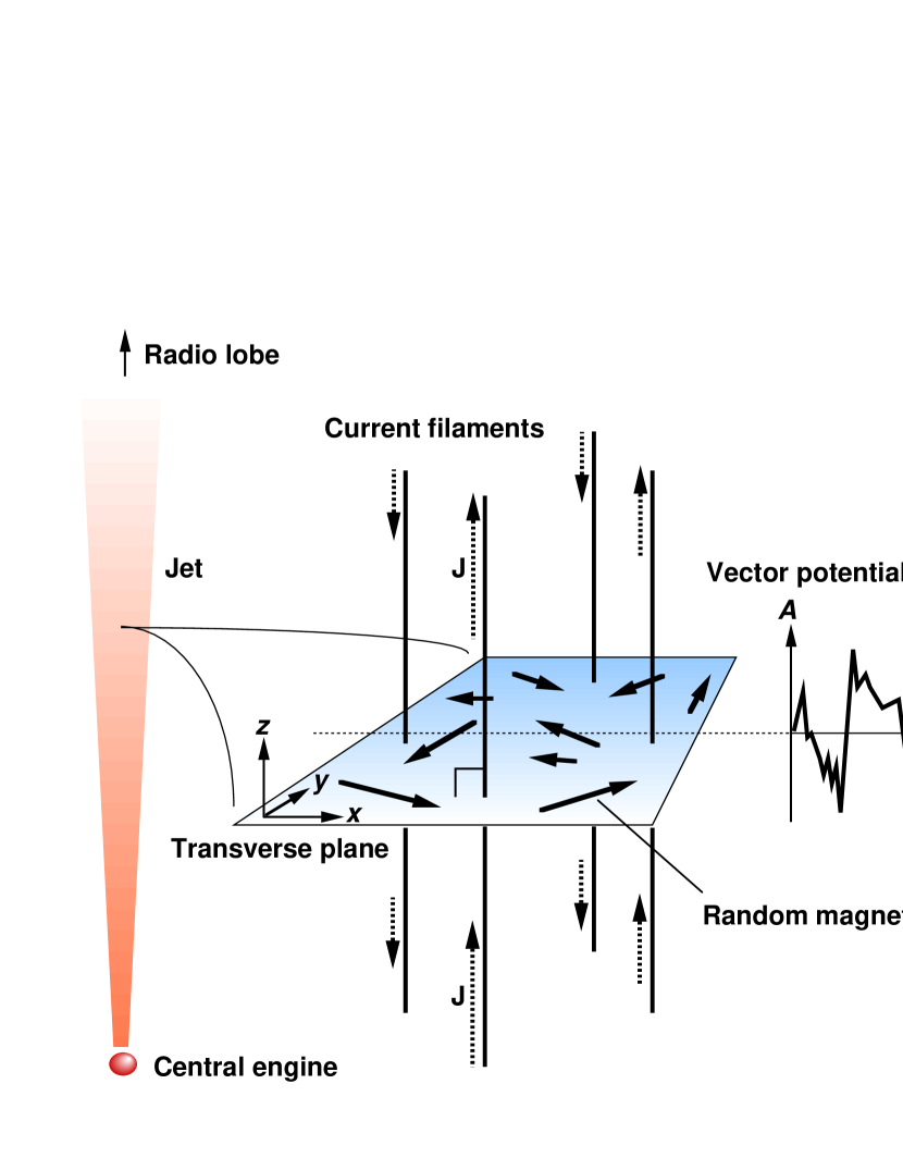
Figure 1: Schematics of the midscale configuration of zeroth-order current density vectors ${\bf J}\sim J{\hat{\bf z}}$ (dotted arrows along the “poles” representing current filaments) and magnetic field vectors ${\bf B}=(B_{x},B_{y},0)$ (bold solid arrows randomly distributed on the shaded plane), and a spatial profile of the vector potential ${\bf A}=A{\hat{\bf z}}$ (bold curve), embodying the magnetized current filaments that constitute the bulk of a large-scale jet. Here the scalar $A(x,y)$ has been depicted as a function of $x$ for a fixed $y$. [See the electronic edition of the Journal for a color version of this figure.]

References

- Abbasi et al. (2004a) Abbasi, R. U., et al. 2004a, Phys. Rev. Lett., 92, 151101
- Abbasi et al. (2004b) ———. 2004b, ApJ, 610, L73
- Aharonian (2002) Aharonian, F. A. 2002, MNRAS, 332, 215
- Appl & Camenzind (1992) Appl, S., & Camenzind, M. 1992, A&A, 256, 354
- Asada et al. (2000) Asada, K., Kameno, S., Inoue, M., Shen, Z.-Q., Horiuchi, S., & Gabuzda, D. C. 2000, in Astrophysical Phenomena Revealed by Space VLBI, ed. H. Hirabayashi, P. G. Edwards, & D. W. Murphy (Sagamihara: ISAS), 51
- Ave et al. (2000) Ave, M., Hinton, J. A., Vázquez, R. A., Watson, A. A., & Zas, E. 2000, Phys. Rev. Lett., 85, 2244
- Bell (1978) Bell, A. R. 1978, MNRAS, 182, 147
- Bell (2004) ———. 2004, MNRAS, 353, 550
- Berezinskiĭ et al. (1990) Berezinskiĭ, V. S., Bulanov, S. V., Dogiel, V. A., Ginzburg, V. L., Ptuskin, V. S. 1990, Astrophysics of Cosmic Rays (Amsterdam: North-Holland)
- Bezler et al. (1984) Bezler, M., Kendziorra, E., Staubert, R., Hasinger, G., Pietsch, W., Reppin, C., Trümper, J., & Voges, W. 1984, A&A, 136, 351
- Bicknell & Begelman (1996) Bicknell, G. V., & Begelman, M. C. 1996, ApJ, 467, 597
- Biermann & Strittmatter (1987) Biermann, P. L., & Strittmatter, P. A. 1987, ApJ, 322, 643
- Biretta et al. (1983) Biretta, J. A., Owen, F. N., & Hardee, P. E. 1983, ApJ, 274, L27
- Biretta et al. (1995) Biretta, J. A., Zhou, F., & Owen, F. N. 1995, ApJ, 447, 582
- Blandford (2000) Blandford, R. D. 2000, Phys. Scr., T85, 191
- Blandford & Eichler (1987) Blandford, R. D., & Eichler, D. 1987, Phys. Rep., 154, 1
- Blandford & Ostriker (1978) Blandford, R. D., & Ostriker, J. P. 1978, ApJ, 221, L29
- Bohm (1949) Bohm, D. 1949, in The Characteristics of Electrical Discharges in Magnetic Fields, ed. A. Guthrie & R. K. Wakerling (New York: McGraw-Hill), 77
- Burbidge (1956) Burbidge, G. R. 1956, ApJ, 124, 416
- Capetti et al. (1997) Capetti, A., Macchetto, F. D., Sparks, W. B., & Biretta, J. A. 1997, A&A, 317, 637
- Carilli & Barthel (1996) Carilli, C. L., & Barthel, P. D. 1996, A&A Rev., 7, 1
- Conway et al. (1993) Conway, R. G., Garrington, S. T., Perley, R. A., & Biretta, J. A. 1993, A&A, 267, 347
- de Marco et al. (2003) de Marco, D., Blasi, P., & Olinto, A. V. 2003, Astropart. Phys., 20, 53
- Drury (1983) Drury, L. O’C. 1983, Rep. Prog. Phys., 46, 973
- Farrar & Biermann (1998) Farrar, G. R., & Biermann, P. L. 1998, Phys. Rev. Lett., 81, 3579
- Gabuzda (1999) Gabuzda, D. C. 1999, New A Rev., 43, 691
- Gaisser (1990) Gaisser, T. K. 1990, Cosmic Rays and Particle Physics (Cambridge: Cambridge Univ. Press)
- Gastaldello & Molendi (2002) Gastaldello, F., & Molendi, S. 2002, ApJ, 572, 160
- Greiner et al. (2003) Greiner, J., et al. 2003, Nature, 426, 157
- Greisen (1966) Greisen, K. 1966, Phys. Rev. Lett., 16, 748
- Heinz & Begelman (1997) Heinz, S., & Begelman, M. C. 1997, ApJ, 490, 653
- Heitler (1954) Heitler, W. 1954, The Quantum Theory of Radiation (London: Oxford Univ. Press)
- Hillas (1984) Hillas, A. M. 1984, ARA&A, 22, 425
- Honda (2000) Honda, M. 2000, Phys. Plasmas, 7, 1606
- Honda (2004) ———. 2004, Phys. Rev. E, 69, 016401
- Honda & Honda (2002) Honda, M., & Honda, Y. S. 2002, ApJ, 569, L39
- Honda & Honda (2004a) ———. 2004a, ApJ, 617, L37
- Honda et al. (2000a) Honda, M., Meyer-ter-Vehn, J., & Pukhov, A. 2000a, Phys. Plasmas, 7, 1302
- Honda et al. (2000b) ———. 2000b, Phys. Rev. Lett., 85, 2128
- Honda & Honda (2004b) Honda, Y. S., & Honda, M. 2004b, ApJ, 613, L25.
- Jokipii (1987) Jokipii, J. R. 1987, ApJ, 313, 842
- Jones & Ellison (1991) Jones, F. C., & Ellison, D. C. 1991, Space Sci. Rev., 58, 259
- Junor et al. (1999) Junor, W., Biretta, J. A., & Livio, M. 1999, Nature, 401, 891
- Kataoka et al. (1999) Kataoka, J., et al. 1999, ApJ, 514, 138
- Kazimura et al. (1998) Kazimura, Y., Sakai, J. I., Neubert, T., & Bulanov, S. V. 1998, ApJ, 498, L183
- Kobayashi (2004) Kobayashi, C. 2004, MNRAS, 347, 740
- Kolmogorov (1941) Kolmogorov, A. N. 1941, CR Acad. Sci. URSS, 30, 301
- Kotani et al. (1996) Kotani, T., Kawai, N., Matsuoka, M., & Brinkmann, W. 1996, PASJ, 48, 619
- Kraichnan (1965) Kraichnan, R. H. 1965, Phys. Fluids, 8, 1385
- Krymskii (1977) Krymskii, G. F. 1977, Soviet Phys. Dokl., 22, 327
- Lagage & Cesarsky (1983a) Lagage, P. O., & Cesarsky, C. J. 1983a, A&A, 118, 223
- Lagage & Cesarsky (1983b) ———. 1983b, A&A, 125, 249
- Landau & Lifshitz (1981) Landau, L. D., & Lifshitz, E. M. 1981, Physical Kinetics (Oxford: Pergamon)
- Lee & Lampe (1973) Lee, R., & Lampe, M. 1973, Phys. Rev. Lett., 31, 1390
- Lobanov & Zensus (2001) Lobanov, A. P., & Zensus, J. A. 2001, Science, 294, 128
- Longair (1992) Longair, M. S. 1992, High Energy Astrophysics, Vol.1: Particles, Photons and Their Detection (Cambridge: Cambridge Univ. Press)
- Lyutikov & Blandford (2003) Lyutikov, M., & Blandford, R. D. 2003, preprint (astro-ph/0312347)
- Matthaeus et al. (2003) Matthaeus, W. H., Qin, G., Bieber, J. W., & Zank, G. P. 2003, ApJ, 590, L53
- Medvedev & Loeb (1999) Medvedev, M. V., & Loeb, A. 1999, ApJ, 526, 697
- Meisenheimer et al. (1989) Meisenheimer, K., Röser, H.-J., Hiltner, P. R., Yates, M. G., Longair, M. S., Chini, R., & Perley, R. A. 1989, A&A, 219, 63
- Meisenheimer et al. (1996) Meisenheimer, K., Röser, H.-J., & Schlötelburg, M. 1996, A&A, 307, 61
- Montgomery & Liu (1979) Montgomery, D., & Liu, C. S. 1979, Phys. Fluids, 22, 866
- Mücke & Protheroe (2001) Mücke, A., & Protheroe, R. J. 2001, Astropart. Phys., 15, 121
- Mücke et al. (2003) Mücke, A., Protheroe, R. J., Engel, R., Rachen, J. P., & Stanev, T. 2003, Astropart. Phys., 18, 593
- Nishikawa et al. (2003) Nishikawa, K.-I., Hardee, P., Richardson, G., Preece, R., Sol, H., & Fishman, G. J. 2003, ApJ, 595, 555
- Novak et al. (2003) Novak, G., et al. 2003, ApJ, 583, L83
- Olinto (2000) Olinto, A. V. 2000, Phys. Rep., 333, 329
- Ostrowski (1988) Ostrowski, M. 1988, MNRAS, 233, 257
- Owen et al. (1990) Owen, F. N., Eilek, J. A., & Keel, W. C. 1990, ApJ, 362, 449
- Owen et al. (1989) Owen, F. N., Hardee, P. E., & Cornwell, T. J. 1989, ApJ, 340, 698
- Perley et al. (1984) Perley, R. A., Dreher, J. W., & Cowan, J. J. 1984, ApJ, 285, L35
- Potash & Wardle (1980) Potash, R. I., & Wardle, J. F. C. 1980, ApJ, 239, 42
- Rachen & Biermann (1993) Rachen, J. P., & Biermann, P. 1993, A&A, 272, 161
- Rawlings & Saunders (1991) Rawlings, S., & Saunders, R. 1991, Nature, 349, 138
- Reid et al. (1989) Reid, M. J., Biretta, J. A., Junor, W., Muxlow, T. W. B., & Spencer, R. E. 1989, ApJ, 336, 112
- Risse et al. (2004) Risse, M., Homola, P., Gora, D., Pekala, J., Wilczynska, B., & Wilczynski, H. 2004, Astropart. Phys., 21, 479
- Silva et al. (2003) Silva, L. O., Fonseca, R. A., Tonge, J. W., Dawson, J. M., Mori, W. B., & Medvedev, M. V. 2003, ApJ, 596, L121
- Stecker & Salamon (1999) Stecker, F. W., & Salamon, M. H. 1999, ApJ, 512, 521
- Takeda et al. (1998) Takeda, M., et al. 1998, Phys. Rev. Lett., 81, 1163
- Tashiro & Isobe (2004) Tashiro, M., & Isobe, N. 2004, Astron. Herald, 97, 400
- Teshima et al. (2003) Teshima, M., et al. 2003, Proc. 28th Int. Cosmic-Ray Conf. (Tsukuba), 437
- Tsytovich & ter Haar (1995) Tsytovich, V. N., & ter Haar, D. 1995, Lectures on Non-linear Plasma Kinetics (Berlin: Springer)
- Vallée (2004) Vallée, J. P. 2004, New A Rev., 48, 763
- Waxman (1995) Waxman, E. 1995, Phys. Rev. Lett., 75, 386
- Webb et al. (1983) Webb, G. M., Axford, W. I., & Terasawa, T. 1983, ApJ, 270, 537
- Wilson & Yang (2002) Wilson, A. S., & Yang, Y. 2002, ApJ, 568, 133
- Yusef-Zadeh et al. (2004) Yusef-Zadeh, F., Hewitt, J., & Cotton, W. 2004, ApJS, 155, 421
- Yusef-Zadeh & Morris (1987) Yusef-Zadeh, F., & Morris, M. 1987, ApJ, 322, 721
- Yusef-Zadeh et al. (1984) Yusef-Zadeh, F., Morris, M., & Chance, D. 1984, Nature, 310, 557
- Zank et al. (2004) Zank, G. P., Li, G., Florinski, V., Matthaeus, W. H., Webb, G. M., & le Roux, J. A. 2004, J. Geophys. Res., 109, A04107
- Zank et al. (1998) Zank, G. P., Matthaeus, W. H., Bieber, J. W., & Moraal, H. 1998, J. Geophys. Res., 103, 2085
-
Zatsepin & Kuzmin (1966)
Zatsepin, G. T., & Kuzmin, V. A. 1966, J. Exp. Theor. Phys. Lett., 4, 78