Investigation of Diffuse Hard X-ray Emission from the Massive Star-Forming Region NGC 6334

Abstract

Chandra ACIS–I data of the molecular cloud and HII region complex NGC 6334 were analyzed. The hard X-ray clumps detected with ASCA (Sekimoto et al., 2000) were resolved into 792 point sources. After removing the point sources, an extended X-ray emission component was detected over a $5\times 9$ pc² region, with the 0.5–8 keV absorption-corrected luminosity of 2$\times 10^{33}$ ergs s^-1 . The contribution from faint point sources to this extended emission was estimated as at most $\sim 20$%, suggesting that most of the emission is diffuse in nature. The X-ray spectrum of the diffuse emission was observed to vary from place to place. In tenuous molecular cloud regions with hydrogen column density of $0.5\sim 1\times 10^{22}$ cm^-2, the spectrum can be represented by a thermal plasma model with temperatures of several keV. The spectrum in dense cloud cores exhibits harder continuum, together with higher absorption more than $\sim 3\times 10^{22}$ cm^-2. In some of such highly obscured regions, the spectrum show extremely hard continua equivalent to a photon index of $\sim 1$, and favor non-thermal interpretation. These results are discussed in the context of thermal and non-thermal emissions, both powered by fast stellar winds from embedded young early-type stars through shock transitions.

1 Introduction

X-rays provide a powerful diagnostic tool of massive star-forming regions (MSFRs). X-ray photons penetrate dense gas and dust cores more deeply than optical and even near infrared lights. Not only serving as a probe, the X-ray emission itself provides evidence that some unexpected energetic processes are operating in MSFRs. Therefore, since the surprising discovery of X-ray emission from the Orion nebula (Giacconi et al., 1974), vigorous X-ray studies on MSFRs have been made with Einstein, ROSAT, and ASCA. Especially, the hard X-ray ($>$ 2 keV) imaging spectroscopy with ASCA has for the first time revealed several clumps in MFSRs, each showing a high temperature (3–10 keV) and a high luminosity (10^32-34 ergs s^-1 ) (e.g., Yamauchi et al. 1996; Hofner and Churchwell 1997; Nakano et al. 2000; Sekimoto et al. 2000). Thanks to its superb angular resolution, these X-ray clumps in MSFRs have been resolved into hundreds of stars with Chandra (e.g., Garmire et al. 2000; Feigelson et al. 2002, 2003; Hofner et al. 2002; Kohno et al. 2002; Nakajima et al. 2003).

Besides individual stars at various evolutionary stages, Chandra first enabled a detailed examination of diffuse X-ray emission in MSFRs. Theoretically, such a phenomenon had long been expected both around individual OB stars (Dyson and de Vries, 1972; Castor et al., 1975; Weaver et al., 1977) as well as in MSFRs (Chevalier and Clegg, 1985). The reported detections of extended soft X-rays ($\lesssim$ 1 keV) associated with MSFRs before Chandra (e.g., the Carina Nebula, Seward and Chlebowski 1982; 30 Doradus nebula in the Large Magelanic Cloud, Wang 1999) were consistent with these predictions. However, even in Galactic MSFRs, it has remained difficult to date to quantify whether the extended X-ray emission really exists, because MSFRs are usually too complex to be resolved by the past X-ray telescopes.

With Chandra, Townsley et al. (2003) indeed reported detections of diffuse soft X-ray emission in two nearby MSFRs, M17 (at a distance of $D=$ 1.6 kpc from the Sun) and the Rosette Nebula ($D=$ 1.4 kpc). They concluded that at least the emission in M17 is diffuse, and explained the phenomenon in terms of stellar-wind shock model (Dyson and de Vries, 1972; Castor et al., 1975; Weaver et al., 1977). Its spectrum was very soft, represented by a two temperature plasma model ($kT=0.13+0.6$ keV). Another Chandra result is the possible detection of diffuse hard X-ray emission from RCW 38 ($D=$ 1.7 kpc; Wolk et al. 2002), which could be of non-thermal origin because a part of the emission show hard continua with a photon index of $1.3\sim 1.6$. Similar phenomena may have also been detected from more distant galactic MSFRs, including the Arches cluster (Wang et al., 2002; Yusef-Zadeh et al., 2002), the Quintuplet cluster (Wang et al., 2002) near the Galactic central, and NGC 3603 at $D=$ 7 kpc (Moffat et al., 2002), although their larger distances make it difficult to remove, even with Chandra, contributions from unresolved point sources.

Thus, the search for diffuse X-ray emission from MSFRs is becoming a new topic explored with Chandra. In the present paper, we describe the analysis of Chandra data of NGC 6334, and report on the discovery of diffuse hard X-ray emission from this representative MSFR.

2 Previous X-ray Results on NGC 6334

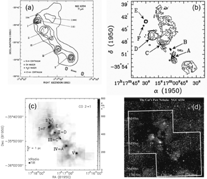
Figure 1: Images of NGC 6334 in; (a) the FIR 71$\mu$m emission (Loughran et al. 1986); (b) radio 18 cm continuum emission (Sarma et al. 2000); (c) CO $J$=2-1 (Kraemer et al. 1999); and (d) NIR (the 2$\mu$m All Sky Survey Atlas image). Roman numerals and Arabic characters designate the FIR cores and HII regions, respectively. In the CO map, crosses and diamonds indicate the positions of the FIR cores and radio peaks. In the NIR map, three colors (blue, green and red) correspond to J (1.2$\mu$m), H (1.6$\mu$m), and K_s (2.2$\mu$m) bands, respectively, and squares indicate the two fields-of-view of the Chandra observations.

NGC 6334 is a nearby ($D=$ 1.7 kpc yielding a plate scale of 1${}^{\prime\prime}=$0.01 pc; Neckel 1978) MSFR, with the bolometric luminosity reaching $L_{\rm bol}\sim 4\times 10^{39}$ ergs s^-1 (Loughran et al., 1986) which is one of the highest of this class. As shown in figure 1, it contains several star-forming sites defined in wide wavelength ranges. Although designations of these sites depend on the observing wavelength, we here follow two commonly used ones; the far-infrared (FIR) cores named I(N), I, II, III, IV, and V (figure 1a); and the radio sources named A, C, D, E, and F (figure 1b). Not all of these are detected in both wavelength ranges (see Kraemer et al. 1999 table 4 for nomenclature). Each site is known to be powered by one or more massive stars, either zero-age main sequence stars (ZAMS) or protostars (e.g., Rodriguez et al. 1982; Harvey and Gatley 1983; Straw et al. 1989). These sites coincide with the dense molecular clouds (figure 1c), the densest part of which appears as the central dark lane in the near-infrared (NIR) map (figure 1d). The central FIR core (III) has no radio masers or outflows that indicate early stages of stellar evolution, but hosts HII regions. It is therefore thought to be most evolved. On the other hand, the FIR cores I, IV and V have outflows and masers, suggesting that the star formation has just started there. The core I (N) has no HII region but masers and an outflow, so that this core is regarded as one of the youngest massive star-forming sites.

In X-rays, NGC 6334 was first detected with the Einstein satellite as 2E1717.1-3548 (Harris et al., 1990), which coincides in position with the FIR core III. With ASCA, Matsuzaki (1999), Matsuzaki et al. (1999) and Sekimoto et al. (2000) found hard X-ray clumps associated with the FIR and radio sources; five FIR cores (I, II, III, IV, and V) were visible in the 2–10 keV band. The region-integrated spectrum exhibits a temperature of 9 keV, which is the highest among the MSFRs observed with ASCA. The X-rays are absorbed by a large absorption column density ($N_{\rm H}\sim 1\times 10^{22}$ cm^-2), suggesting that the emission originates from embedded young massive stars. The region-integrated 0.5–10 keV X-ray luminosity, 6$\times$10³³ ergs s^-1 , makes NGC 6334 one of the most X-ray luminous MSFRs ever observed with ASCA. Thus, NGC 6334 is without doubt an attractive target to search for diffuse hard X-rays, and if detected, to investigate their properties and emission mechanism.

3 Observation and Data Reduction

We conducted two 40 ksec observations of NGC 6334 with Chandra, on 2002 August 31 and 2002 September 2. In order to cover the whole nebula, we placed the aimpoint at the J2000 co-ordinates of (17^h 20^m 53.^s45, $-$35^d 47^m 19.^s33) and (17^h 20^m 00.^s44, $-$35^d 56^m 22.^s26) in the August and September observations, respectively. Hereafter we call the former “north field” and the latter “south field”, according to their declinations. The two fields of view partially overlap (see figure 1 d). The Advanced CCD Imaging Spectrometer (ACIS–I0, I1, I2, I3, S2, and S3) was utilized. In this paper, we analyze only the data from the four ACIS–I chips, because the point spread function (PSF) of the telescope becomes significantly broader at the positions of the ACIS–S chips.

We started data reduction with the Level 1 event files provided by the Chandra X-ray Center, and followed the standard data reduction procedures using the CIAO (Chandra Interactive Analysis of Observations) software package version 2.3 and the calibration data base (caldb) version 2.18. We corrected pulse heights for the charge transfer inefficiency (CTI), and removed the ACIS pixel randomization to improve image quality. No background flares occurred in the north-field observation, while nearly half the south-field exposure was affected by them. We then conducted flare filtering, by excluding those portions where the 0.5–8 keV count rate was $>$1.2 times the quiescent average of the south-field observation ($\sim$4$\times 10^{-7}$ ct s^-1 pixel^-1). We have thus obtained 39.4 and 19.4 ksec exposure times for the north and south observations, respectively.

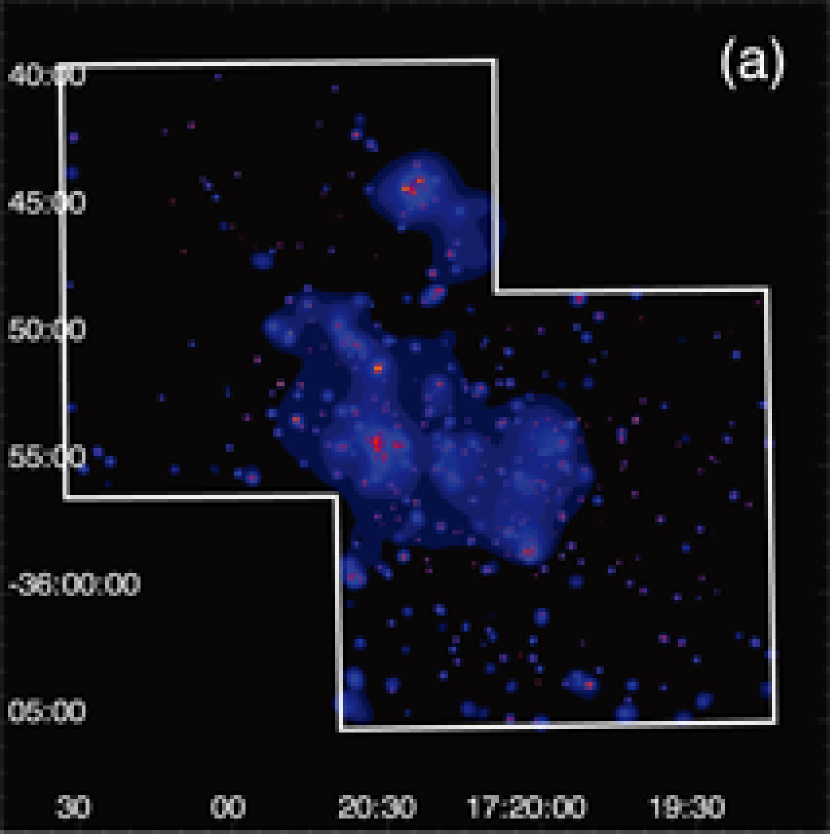
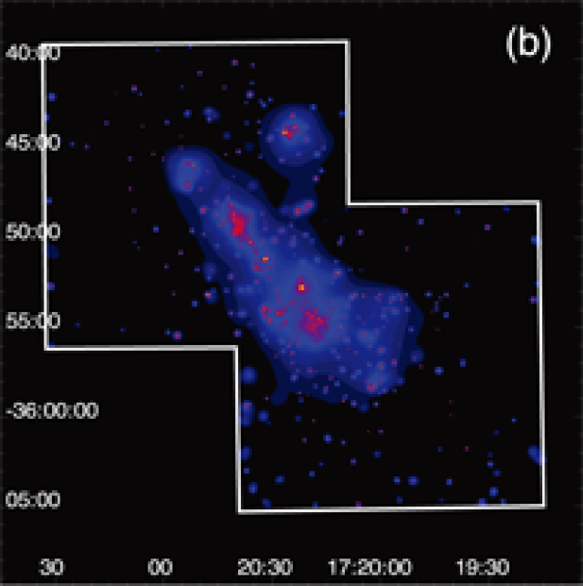
Figure 2: Adaptively smoothed X-ray images of NGC 6334 in the (a) 0.5–2 and (b) 2–8 keV bands, displayed on the J2000 coordinates. They are corrected for the exposure and vignetting, but the background is not subtracted. The CIAO program csmooth is utilized. The two observed fields are merged together. The ACIS–I fields of view are shown in white lines. The intensity is plotted logarithmically from 1.0$\times 10^{-9}$ to 2.9$\times 10^{-6}$ counts s^-1 pixel^-1 cm^-2 in panel (a), while from 1.8$\times 10^{-9}$ to 2.9$\times 10^{-6}$ in panel (b).

Using these data sets, we created X-ray images in the 0.5–2 and 2–8 keV bands, as shown in figure 2. We observe a number of point sources and also indication of extended structures. However, it is not clear at this stage whether they really represent diffuse emission or simply a sum of point sources which cannot be resolved even with Chandra. Therefore, before analyzing the data for suggested extended emission, we conduct point source analysis in the next section.

4 Point Source Analysis

The wavdetect program was utilized to detect point sources (Freeman et al. 2002). We used images in three bands (0.5–2, 2–8, and 0.5–8 keV) independently, in order not to miss very soft or strongly absorbed sources. The significance criterion and wavelet scales were set as 1$\times 10^{-6}$ and 1 to 16 pixels in multiples of $\sqrt{2}$, respectively. As a result, we have detected 449 and 390 sources in the north and south fields, respectively. Among them, 42 sources in the north field have counterparts in the south field within the position-dependent angular resolution, approximately defined in Feigelson et al. (2002). Excluding these overlaps, the total source number becomes 792.

We extracted events of the individual point sources using regions given by the wavdetect program. The background was extracted around each source excluding other point sources, and then scaled to the on-source area. The scaled background counts amount to $\sim$1-8 % of the raw source counts near the aimpoint, while $\sim$20-40 % for sources at $8^{\prime}$. After subtracting the background, the detected sources exhibit net signal counts (hereafter netcounts) of $\sim$2 to 3000. Although faint sources less than $\;\buildrel<\over{\sim}\;$5 netcounts have low significance ($\lower 2.15277pt\hbox{$\;\buildrel<\over{\sim}\;$}2\sigma$), we here take them as possible point sources, in order not to include their counts into the potentially extended emission. We then produced source-number histograms as a function of logarithm of netcounts, in 6 separate annular regions (0-2, 2-4, 4-6, 6-8, 8-10 and $>$10 arcminites from the aimpoint) in each ACIS–I field. Reflecting a roughly power-law like source intensity distribution (see §5.3 for details), the source number first increases toward lower counts, reaches a maximum, and then decreases due to the sensitivity limit. We regard this maximum of the histogram as representing the completeness limit of the point-source detection. In both observations, the completeness limit estimated in this way monotonically increases with the angular distance from $\sim$10 to $\sim$30 netcounts, due to the PSF broadening. When utilizing a typical count-to-flux conversion factor of $\sim 2\times 10^{-11}$ ergs s^-1 cm s^-2 (netcounts/s)^-1 obtained from spectral fitting of the 163 bright ($>30$ netcounts) sources, 10 netcounts corresponds to the 0.5–8 keV X-ray flux of $\sim 0.5\times 10^{-14}$ and $\sim 1\times 10^{-14}$ ergs s^-1 cm s^-2 , in the north and south fields, respectively. At an assumed distance of 1.7 kpc, these fluxes translate to $\sim 2\times 10^{30}$ and $\sim 4\times 10^{30}$ ergs s^-1 . Detailed point source analyses will be presented elsewhere (Ezoe et al. in preparation).

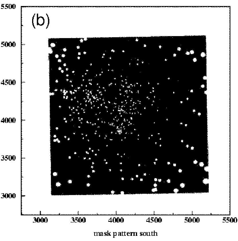
Figure 3: Point-source mask patterns for the (a) north and (b) south field observations, generated using the mask radius given by the ChaRT program.

We have so far utilized signal extraction regions specified by the wavedetect routine. Although these regions are optimum for the source detection, they are usually too small to thoroughly remove photons from the point source. Accordingly, we defined new circular regions around individual sources, based on the “Chandra Ray Tracer” (ChaRT). Specifically, we calculated the encircled-photon fraction as a function of energy and separation angle from the aimpoint (0, 1, 2, 3, 5, 7, 10, and 15 arcminites). For each source, we looked up the results, using interpolation if necessary, and chose a radius to include $\sim 98$ % of photons at the Al K$\alpha$-line energy (1.497 keV). Figure 3 shows point-source mask patterns, obtained by summing up these larger regions around the individual point sources. In this procedure, 8% and 7% of the whole ACIS–I area have been excluded from the north and south field, respectively.

5 Analysis of Extended X-ray Emission

5.1 Images

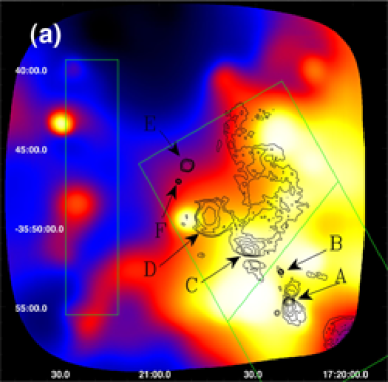
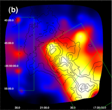
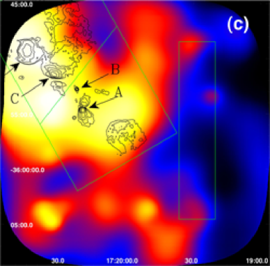
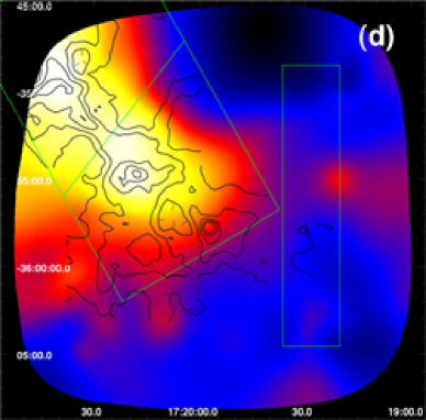
Figure 4: Adaptively smoothed images of the extended emission in the 0.5–2 keV (left) and 2–7 keV (right) bands, obtained by removing point sources using the mask patterns of figure 3. The top and bottom panels correspond to the north and south observations respectively. They are corrected for the exposure and vignetting, but the background is not subtracted. Squares and trapezoids indicate regions utilized in the spectral analysis. Contours indicate the 18 cm radio continuum (Sarma et al. 2000, left) and the CO $J$=2-1 maps (Kraemer et al. 1999, right).

We applied the point-source masks (figure 3) to the raw ACIS images to remove point sources, and then created images of the residual emission using the CIAO tools dmfilth and csmooth. The former fills holes in the image with values interpolated from surrounding regions, and the latter adaptively smoothes the filled image. We utilized default parameters (kernel sizes and significances) in the csmooth routine. We corrected these images for the vignetting and exposure times. Figure 4 shows the images of the residual emission in two energy bands, obtained in this way. To retain the best positional resolution available, we here show the two images separately instead of merging them together. In addition, the energy range is restricted to below 7 keV, to avoid the strong instrumental Ni K$\alpha$ line in the ACIS background.

As is clear from the procedure, the images shown in figure 4 are thought to represent the apparently extended emission noticed in figure 2, although they must be examined carefully against possible contribution from fainter (and hence individually undetectable) point sources. The overlapping region appears in somewhat different ways between the north and south field images. This is due to the position-dependent angular resolution as described in §4.

5.2 Spectrum

5.2.1 Region definition

In order to analyze the spectrum of the extended emission, we define in figure 4 a rectangle of $\sim 10^{\prime}\times 18^{\prime}$, elongated along the linearly aligned cores, and call it “extended emission region”, or EER for short. Using the equilateral line from the two aimpoints, we further subdivide this EER into two trapezoids. When analyzing the north-eastern and south-western trapezoids, we use only the north and south field observation data, respectively. This ensures that the overlapping region is always placed within $\sim 8^{\prime}$ of either of the two aimpoints.

Because NGC 6334 is located on the Galactic plane, it is contaminated by the diffuse emission along the Galactic ridge (e.g., Kaneda et al. 1997; Valinia and Marshall 1998; Ebisawa et al. 2001). In order to remove this unwanted component, we need to subtract local background rather than those from blank skies. We have therefore chosen two square background regions where the extended emission is relatively weak (see figure 4). Hereafter we collectively call them “background region” or BR for short, and utilize the events summed over them as our background. The total area of the EER is 2.80/2.55$\times 10^{6}$ pixel² before/after excluding the areas around point sources. These areas correspond to 191/174 arcmin² or 47/43 pc² in 1.7 kpc. Thus, the excluded area is $\sim$10 %. Similary, those of the BR are 1.57/1.50$\times 10^{6}$ pixel².

We then extracted spectra from the EER. The weighted arf and rmf files were calculated using the CIAO programs mkwarf and mkwrmf, respectively, which take account of position-dependent detector responses such as vignetting and energy resolution. The apply_acisabs script was utilized when creating arf files, to correct them for the recent decrease in the ACIS quantum efficiency. We thus obtained two sets of spectrum, arf, and rmf files corresponding to the two observations, and then added them together considering the difference in their exposure times. In this way, we have acquired the combined spectrum of the EER. We similarly derived a background spectrum from the BR. Below, we utilize them after normalizing to the detector area (pixel²), excluding the removed point sources. Since the effective area (cm²) and also the instrumental background varies from place to place within ACIS–I, we must consider the positional difference of the sky and non X-ray backgrounds between the EER and BR. In the next section, we hence examine the excess emission considering these uncertainties.

5.2.2 Excess emission

Figure 5 (a) compares the spectrum of the EER with that derived from the BR, both normalized to the same detector area. The former is higher than the latter by a factor of two in the 2–5 keV range, while they agree in energies below 0.7 keV and above 7 keV where the instrumental background is dominant. The 0.5–7 keV raw counts of the EER and BR spectra are 22,500$\pm$150 and 14,600$\pm$160, respectively, yielding the excess counts of 7,900$\pm$220. Thus, the excess emission is statistically quite significant.

To further confirm the significance of the extended emission, we investigated the systematic uncertainties in the background. First, we compared the 5–10 keV count rates of two blank-sky spectra, extracted from the EER and BR locations of a blank-sky observation available to us, and examined the instrumental background for any position dependence. We found negligible ($\sim$1 %) difference between the two detector regions. Second, to examine how much the vignetting effect affects the amount of the sky background (Galactic ridge emission and cosmic X-ray background), we compared effective areas of the EER and BR specified by their response files. The BR area was found to be smaller than the EER area by $\sim$5% at $<$5 keV, and by $\sim 15$% at 7 keV; the resultant increase of the sky background is only 4% of the extended emission. Thus, the excess counts in the EER can be concluded to be significant even considering systematic errors.

5.2.3 Comparison with summed point sources

In order to characterize the spectrum of the background-subtracted EER emission, we compare it in figure 5 (b) with the ACIS spectrum summed over the 548 point sources detected within the EER. This figure immediately reveals several important features of the extended emission. Firstly, it is nearly half as luminous as the emission summed over all the detected point sources. Secondly, the extended emission exhibits a harder spectral continuum in the 2–7 keV range. Third, no significant emission line is observed in the EER spectrum, in contrast to the point-source spectrum which shows several emission lines from elements such as S, Ar, and Fe. (Incidentally, the simultaneous presence of these lines is not surprising, since we have added sources with various temperatures). In order to better visualize this, we show the ratio of the two spectra in figure 5 (c). By fitting the spectral ratios with a linear function of energy, given as ($A_{0}+A_{1}\times$Energy), we obtained $A_{0}=0.38\pm 0.03$ and $A_{1}=0.043\pm 0.012$ where errors are 1$\sigma$. The two spectra significantly differs each other.

5.2.4 Flux and luminosity

We conducted spectral fitting to the EER spectrum, to quantify its basic properties such as the X-ray flux and luminosity. We here employed a simple power-law model with an interstellar absorption. Here and hereafter, all quoted errors in the spectral fitting refer to 90 % confidence levels unless otherwise stated. Table 1 lists the obtained parameters, and figure 6 (a) shows the fitting results. The fit was not acceptable with $\chi^{2}/\nu\sim 2$ because of an excess around 2–3 keV, although it contributes only $\sim$5% in the 0.5–7 keV flux. The 0.5–8 keV flux implied by the best-fit model is 5.6$\times 10^{-12}$ ergs s^-1 cm s^-2 before removing the absorption, and the absorption-corrected 0.5–8 keV luminosity reaches 2$\times 10^{33}$ ergs s^-1 .

For comparison, we quantified the summed point-source spectrum in terms of a power-law model. Additionally, three Gaussians were utilized to reproduce the H-like Si K_β (line1), He-like Ar K_α (line2), and a complex of neutral and He-like Fe K_α (line3) lines, seen in the spectrum. We obtained results as shown in table 2 and figure 6 (b); the relatively hard continuum ($\Gamma\sim 1.2$) is considered to arise from a superposition of plasma emission absorbed with different column densities.

We also consider to what extent the EER spectrum is contaminated by photons which escaped from the summed point sources. We then multiplied the above model for the summed point sources by the escape-fraction curve estimated by the ChaRT program, and re-fitted the EER spectrum considering this contribution. This has little changed the results, except an $\sim$10% decrease of the EER flux. Thus, the contamination of the detected point sources is small.

5.3 Luminosity Function

The Chandra data of NGC 6334 thus reveal an apparently extended hard X-ray emission, which remains significant after removing the detected point sources. Although this emission could be truly diffuse, it could alternatively be formed by a collection of faint point sources which are individually undetectable. In order to examine this issue, we utilize the luminosity function of the detected point sources. Here we define it by a cumulative column number density (pc^-2) of those sources of which the absorption-uncorrected 0.5–8 keV luminosity is higher than a specified value, $L$ (ergs s^-1 ).

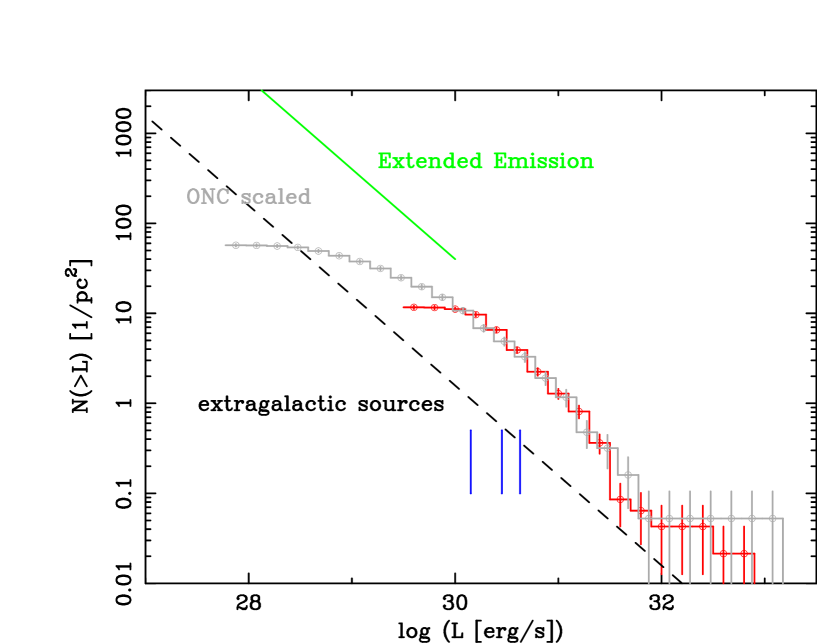
Figure 7: The luminosity function of the point sources within the EER (red), compared with that of ONC (gray) taken from Feigelson et al. (2002). The vertical axis is the column density of the source number, while the horizontal axis absorption-uncorrected 0.5–8 keV luminosity. The ONC curve is scaled considering absorption and source density (see text). Errors are 1$\sigma$ Poisson. The green line indicates the number of putative point sources at a given flux that can account for the observed total surface brightness of the extended emission. Three vertical lines near the bottom are the typical X-ray fluxes of point sources yielding 10, 20, and 30 netcounts in a 40 ksec observation. The dashed line indicates the expected number of extragalactic sources.

Figure 7 shows the luminosity function of the 548 point sources in the EER; we derived $L$ of the bright sources ($\geq$30 netcounts) by spectral fitting. We fitted each spectrum with a plasma emission code called apec (astrophysical plasma emission code) or power-law model, whichever gives a better fit to the data. Details will be presented in Ezoe et al. (in preparation). For the other faint sources ($<$ 30 netcounts), we utilized the count-to-flux conversion factor derived from the summed point sources (figure 6 b); $\sim 2\times 10^{-11}$ ergs s^-1 cm s^-2 (netcounts/s)^-1.

In figure 7, the source number density increases toward lower luminosities, and saturates below $\sim 10$ netcounts, corresponding to the completeness limit estimated in §4. Specifically, the completeness limit becomes about 30 netcounts/(40 ksec), or $5\times 10^{30}$ ergs s^-1 in terms of absorption-uncorrected 0.5–8 keV luminosity. Then, in order to complement the luminosity function below this limit, we have incorporated Chandra results on the Orion Nebula Cluster (ONC) by Feigelson et al. (2002), which also utilize an absorption-uncorrected luminosity function. This is a representative and very nearby ($D=450$pc) MSFR, and the completeness limit of Feigelson et al. (2002), in terms of the 0.5–8 keV luminosity, is lower by a factor of 20 than the present limit for NGC 6334. Furthermore, the stellar mass function of NGC 6334 and that of the Orion Nebula are known to have consistent shapes within errors, as indicated by NIR observations (Straw et al., 1989). Another justification for using the ONC result is provided by the fact that nearby young stellar clusters have very similar low-mass stellar populations, and hence similar X-ray luminosity functions toward the low-luminosity end (Feigelson and Getman, 2004). Therefore, the ONC result is ideal for interpolating the luminosity function of NGC 6334 below our detection limit.

To be more accurate, we would have to compare the two luminosity functions after correcting for the absorption. Considering this, we scaled that of ONC by a factor of 1.3 toward lower luminosities, because typical column densities in ONC and NGC 6334 are $\sim 0.5\times 10^{22}$ and $\sim 1.3\times 10^{22}$ cm^-2, respectively (Feigelson et al. 2002; Dickey and Lockman 1990), and hence a typical YSO with $kT\sim 3$ keV would be subject to a larger correction for absorption if it is in NGC 6334 than in ONC. In the vertical direction, we arbitrarily scaled the luminosity function of ONC by a factor of 0.3, so that it coincides with that of NGC 6334 at the luminosity of the completeness limit. This scaling factor, $<1$, is consistent with the fact that the EER contains not only star-forming cores but also molecular cloud envelopes; the EER contains $\sim$7 star-forming cores in 47.1 pc², while ONC has 1 in 4.9 pc². Thus, the stellar density must be higher in ONC. After these shifts, the two luminosity functions coincide with each other very well within Poisson errors, in luminosities above $5\times 10^{30}$ ergs s^-1 . This reconfirms that the X-ray source population is similar between these two objects, and that the estimation of the completeness limit is reliable.

We estimated the expected flux of unresolved sources by integrating the rescaled ONC luminosity function, from the completeness limit down to the end, $\sim 10^{28}$ ergs s^-1 . From this, we subtracted the number of point sources actually detected in our observations at luminosities below the completeness limit. Then, the estimated unresolved sources have turned out to be 2500 in number, and $\sim 0.5\times 10^{31}$ erg s^-1 pc^-2 in surface brightness. This is only 12 % of the value needed to account for the surface brightness of the extended emission. We further extrapolated the function into 0 ergs s^-1 assuming a slope of 0.4, taken from that of ONC in the 10^29-30 ergs s^-1 range; we found that it reaches at most $\sim$20 %, and hence falls still short of the extended emission.

In order to estimate the expected flux from the background extragalactic sources, we utilized the source density from Giacconi et al. (2001). We converted the flux into the luminosity, and the surface number density of sources into their column density, both assuming that all of them are at the distance of NGC 6334. The flux estimated in this way is negligible (3% in $10^{27}-10^{28}$ ergs s^-1 ). Furthermore, the strong concentration of the extended emission on the EER cannot be explained by background objects.

In conclusion, a large part ($\lower 2.15277pt\hbox{$\;\buildrel>\over{\sim}\;$}80$%) of the extended emission is suggested to be truly diffuse in nature. The spectral difference between the diffuse emission and the point sources (§5.2.3, fig 5 c) independently supports this conclusion.

6 Region-by-region Spectral Analysis

Although the apparently flat continuum of the EER, represented by a power-law index of 0.9, is suggestive of non-thermal emission, such a flat continuum could alternatively be produced by a superposition of thermal components with different absorptions. Accordingly, in this section, we divide the EER into finer regions, and study the spectrum and X-ray absorption as a function of the position.

6.1 Region selection

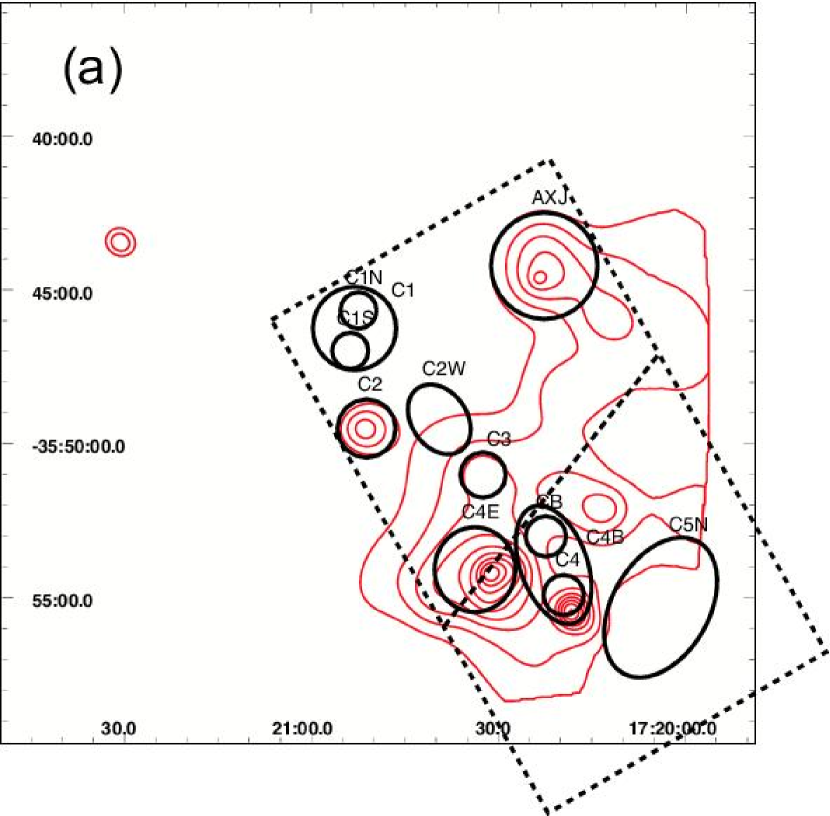
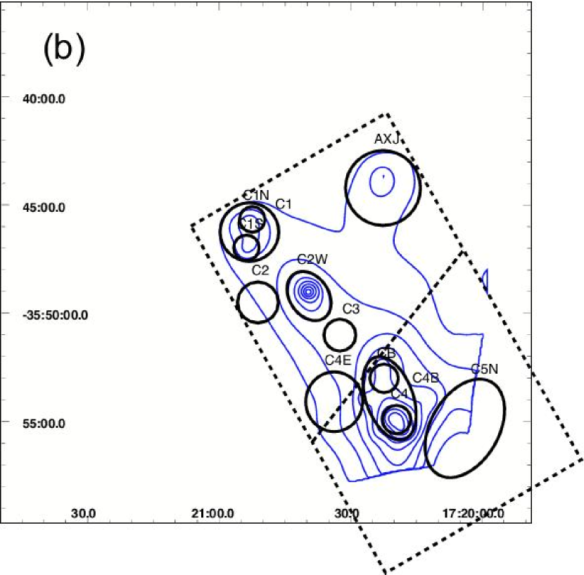
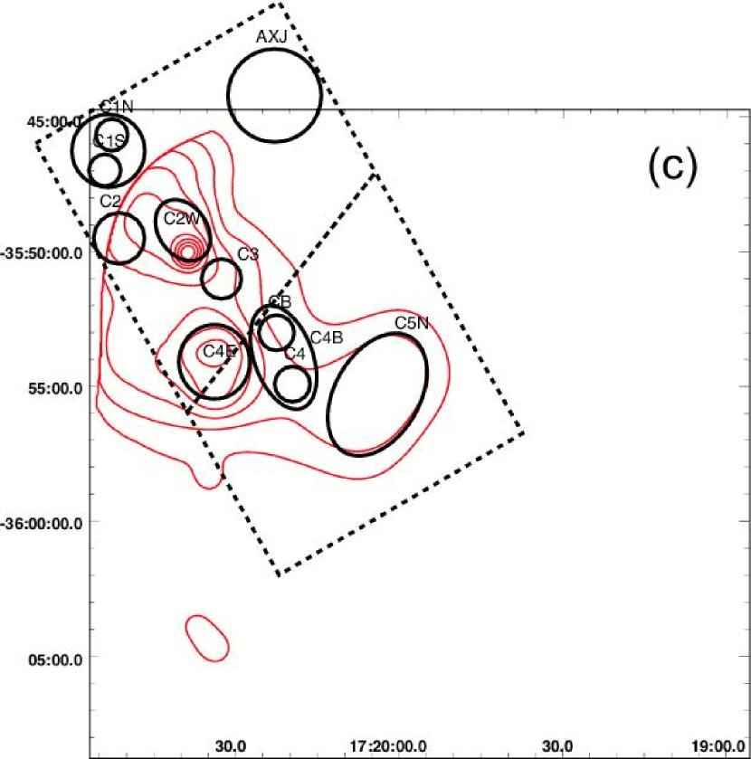
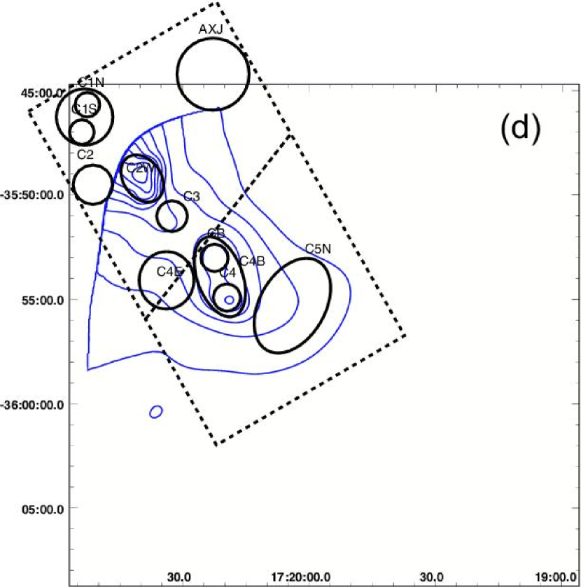
Figure 8: The same as figure 4 but plotted with contours in logarithmic scales. Panels (a) and (c) show the soft band images, while (b) and (d) those in the hard band. Panels (a) and (b) represent the north field while (c) and (d) the south field. Solid circles and ellipses indicate the selected regions to be utilized in the spectral analysis. Two dashed trapezoids represent the EER.

To conduct the spatially-resolved spectroscopy, we have reproduced in figure 8 the two-band images of figure 4, but utilizing this time logarithmic contour representations. The contours are separated by a factor of 1.1 and 1.2 in the background-inclusive brightness in the soft and hard band images, respectively, while the lowest contour represents $\sim$1.3 times the average BBR value in both bands. In reference to these two-band images, let us define characteristic regions, particularly bright clumps, to be utilized in the subsequent analysis.

Figure 8 (a), namely the soft X-ray image of the north field, reveals several bright clumps coincident with the FIR cores or the condensations of massive stars. Referring to this contour map, we then define three circular regions, named C2, C3, and AXJ, with C standing for “FIR core” and AXJ the known X-ray source AXJ 1720.4$-$3544 which is identified with a B0.5e star by Matsuzaki (1999). The C3 region is less clear than the other two, but it is chosen so as to include the known massive ZAMS (O8) at its center.

In the hard X-ray image of the north field (figure 8 b), these three regions become less clear. On the other hand, a bright clump emerges at the position of the FIR core I(N) and I. Accordingly, a new region C1 is defined, together with two more sub-regions in it, C1N and C1S to represent the two independent FIR cores therein. Also, a significant emission can be seen to the west of the FIR core II, coincident with a molecular cloud dark lane and a condensation of embedded stars. Hence, we define another region named C2W region. After all, we have defined 7 regions in the north field (C1, C1N, C1S, C2, C2W, C3, and AXJ).

Similarly, using figure 8 (c) which is the soft X-ray map of the south field, we select two bright soft X-ray regions, C4E and C5N, toward the east and north directions of the core IV and V, respectively. In the hard X-ray map (figure 8 d), a bright clump stand out at the FIR core IV and its north position, which are covered by regions named C4 and CB, respectively. A larger region C4B is employed to sum up C4 and CB. Thus, in the south field, we have defined 5 regions (C4E, C5N, C4, CB and C4B). After all, the EER has been subdivided into 12 representative regions.

6.2 Color-color diagram

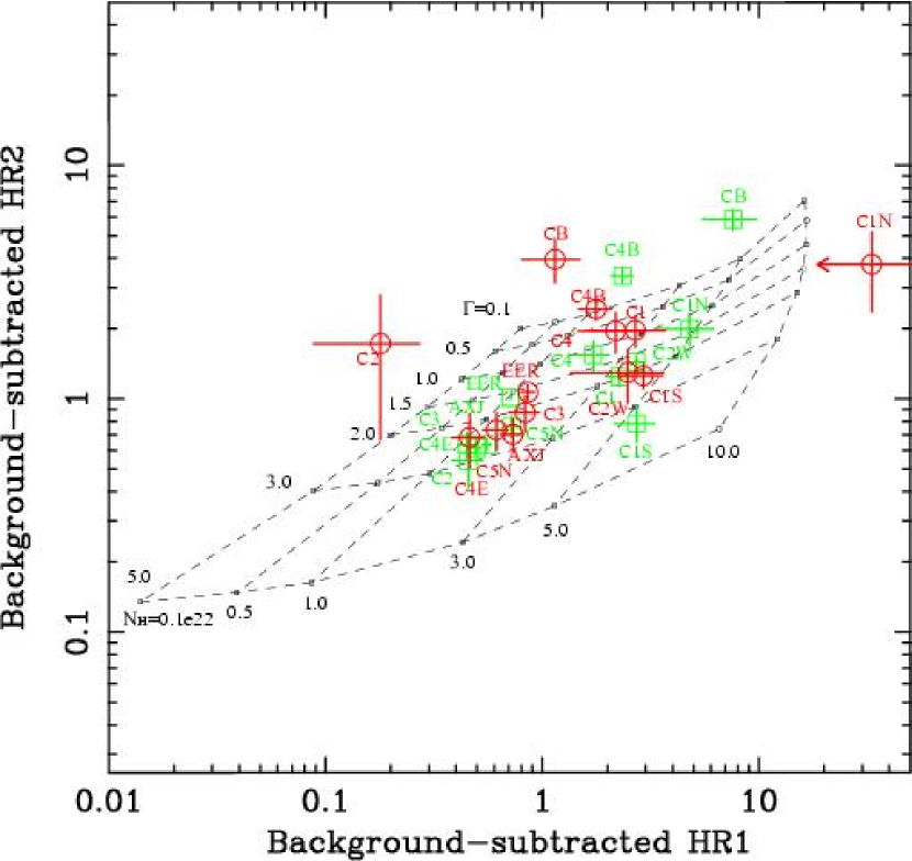
Figure 9: The color-color diagram of the diffuse emission (red) and the summed point sources therein (green), measured in the 12 regions defined in figure 8. The error bars represent $\pm 1\sigma$ statistical uncertainties. Dashed lines are predictions by a family of single power-law models, having different power-law indicies and suffering different interstellar absorptions in a unit of 10²² cm^-2.

To grasp the spectral properties of the 12 regions, we arranged them in figure 9 on a color-color diagram. We divide the 0.5–7 keV band into three finer bands ($S$ 0.5–2.0, $M$ 2.0–3.5, and $H$ 3.5–7 keV), and created two hardness ratio maps by calculating $HR_{1}=M/S$ and $HR_{2}=H/M$. $HR_{1}$ is expected to mainly reflect a difference in an absorption column density, while $HR_{2}$ is more sensitive to the intrinsic continuum hardness. The data points can be clearly subdivided into two groups; (1) ”soft” regions with $HR_{1}\lesssim 1$ and $HR_{2}\lesssim 1$, including AXJ, C2, C3, C4E and C5N; and (2) ”hard” regions with $HR_{1}\gtrsim 1$ and $HR_{2}\gtrsim 1$, including C1, C1N, C1S, C2W, C4, CB, and C4B.

For comparison, green points in figure 9 show the hardness ratios of the summed point sources in the individual regions. The green data are again divided into the two groups; the point sources in the soft regions exhibit smaller values of $HR_{1}$ than those in the hard ones. The $HR_{2}$ values are also different between the two groups, especially in CB and C4B, although these two are contaminated by the bright background AGN (NGC 6334 B). Importantly, most of these summed point sources have similar or even higher values of $HR_{1}$ than the diffuse emission in the same region, suggesting that the latter suffers less absorption.

6.3 Spectral fitting for summed point sources

Before analyzing the diffuse emission spectra, we analyze spectra of the summed point sources with two aims in mind. One is to estimate their absorption column densities, which serve as a measure of absorption affecting the diffuse emissions. The other is to utilize their spectral shapes to estimate the effects of those photons which escape from the point sources into the diffuse emission.

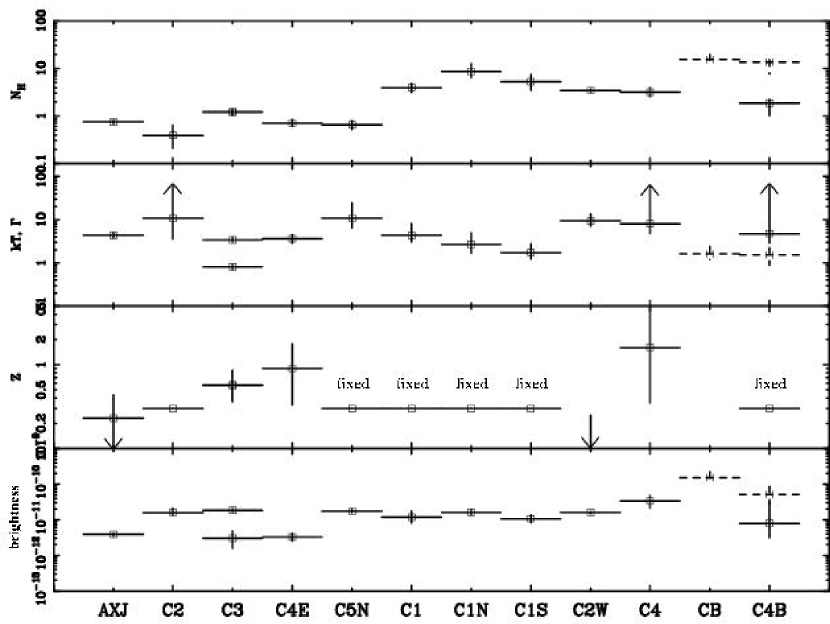
Figure 10: Results of the spectral fitting to the summed point sources in the 12 diffuse emission regions with a single temperature (plus Gaussian) model, or a power-law model (dashed), or a combination of them. From top to bottom panels, plotted are the best-fit values of the absorption column density in 10²² cm^-2, the temperature in keV or photon index, the abundance in solar units, and the uncorrected 0.5–8 keV X-ray surface brightness in ergs s^-1 cm s^-2 pc^-2.

In the same way as in §5.2.3, we prepared the spectrum of the summed point sources in each region, and fitted it with simple models. The spectra in 8 out of the 12 regions have been represented successfully by a single temperature thin-thermal model. The C2W and C3 region required an additional narrow Gaussian and a second thermal plasma model of a rather low temperature, respectively. For the remaining two regions (CB and C4B) which involve the bright AGN (NGC 6334 B), a power-law model and a single temperature plus power-law model, respectively, gave acceptable fits. All the 12 spectra have been successfully reproduced in this way, yielding the results in figure 10.

The obtained absorption column density differs clearly between the soft and hard regions, confirming the inference from the color-color diagram. Specifically, the soft regions have column densities of $(0.5\sim 1)\times 10^{22}$ cm^-2, while the hard ones have $(2\sim 10)\times 10^{22}$ cm^-2. These values are consistent (within a factor of $\sim 3$) with those values estimated in other wavelength ranges, such as the radio CO line (Kraemer et al., 1999) and NIR extinctions (Straw et al., 1989). Furthermore, every spectrum except those from three regions (C3, CB and C4B) has been successfully reproduced by a single temperature plasma model absorbed by a single column density. This ensures that each of the 12 regions has a well-defined value of $N_{\rm H}$. The derived temperatures are moderately high, i.e., several keV, in agreement with the typical X-ray temperature of YSOs. Therefore, the detected point sources can be mostly understood as YSOs suffering from region-dependent absorptions.

6.4 Spectral fitting of the diffuse emission

We then conducted model fitting to the diffuse emission spectrum in each region. In the same way as the EER analysis (§5.2.4), the escape photons from the summed point sources were taken into account by adding their best-fit models, after multiplying with the third-order polynomial function. Unlike the EER case as a whole, this effect is significant ($\sim$20-30% of the diffuse emission in 0.5–7 keV) in a few regions (AXJ, C3, and CB) hosting very bright X-ray sources ($\;\buildrel>\over{\sim}\;$ 1000 netcounts).

6.4.1 Soft regions

We fitted the spectra of the 5 soft regions with a single temperature plasma model. The temperature and the column density were left free to vary, while the heavy element abundances were fixed at 0.3 solar. Results are shown in figure 11, and the derived parameters are listed in table 3. Thus, the fits have been acceptable in all the 5 cases.

As expected from the color-color diagram, all the 5 spectra show relatively low absorption column densities, in the range of $0.4\sim 1.1\times 10^{22}$ cm^-2. The measured absorption agrees, within respective errors, with that of the summed point sources in the same region. The estimated temperatures range from 1 (C2) to 9 keV (C5N), except that in C3 which is not well constrained. The region C3 needs some caution, because its surface brightness is rather low (figure 8a), its diffuse-emission temperature is not well determined (table 3), and its point-source spectrum requires an additional softer continuum (figure 10). Therefore, the absorption column density in this region may still take multiple values.

6.4.2 Hard regions

In the same way, we fitted all the 7 hard-region spectra with a single temperature model. Because photon statistics in the soft X-ray band are rather limited and the $HR_{1}$ in the color-color diagram (figure 9) are similar between the diffuse emission and the summed point sources, we fixed the absorption column densities at those of the summed point sources ($3.5\sim 8.8\times 10^{22}$ cm^-2, see the first line in table 4), except in the C4B region in which we left $N_{\rm H}$ free to vary. The abundance was fixed at 0.3 solar, except in C1 and C1S for which it was left free to reproduce a sign of Fe-K line emission.

The results of this analysis are shown in figure 12 and table 4. All the fits have been acceptable, although that of C4B fit is marginal ($\chi^{2}/\nu\sim 1.4$) because of the data excess in 1–2 keV. As already suggested by the color-color diagram, the diffuse continua in the hard regions are generally flatter than those in the soft regions. Nevertheless, the C1, C1N, C1S and C2W spectra could still be regarded as dominated by thin thermal emission, because the obtained temperatures (5$\sim$10 keV) are not unusual among cosmic hot plasmas, and the C1 spectra (and possibly C1S spectra too) shows the emission feature attributable to Fe-K lines.

Among the four spectra (C1, C1N, C1S, and C2W) with reasonable temperatures, those of C1N, C1S, and C2W show reasonable abundances (solar or sub-solar). However, the C1 spectrum requires a very high ($>$1.9 solar) abundance, because of the strong Fe-K line. If the spectrum is fitted by a phenomenological model consisting of a power-law continuum and a Gaussian, the line center energy is obtained as 6.7${}_{-0.2}^{+1.0}$ keV, with the intrinsic line width of 180 ($<830$) eV and an equivalent width was as huge as 1.5 keV. The center energy implies a highly ionized Fe-K line. Then, if we naturally interpret the C1N spectrum as thermal emission, the large equivalent width may be due to a high local abundance. On the other hand, as suggested in the Galactic ridge X-ray Emission (Masai et al., 2002), the hard continuum of C1N and also the Fe K-line may partially be quasi-thermal, i.e., arising from Coulomb collisions of accelerated (non-thermal) electrons with thermal ions. This quasi-thermal component can create an apparently thermal spectrum of several keV and increase the equivalent width of the ionized Fe-K line. Hence, we cannot reject this non-thermal possibility for the C1N spectrum.

The remaining three spectra (C4, CB, and C4B) lack emission lines and exhibit very flat continua, requiring $kT>10$ keV if adopting thermal interpretation. Such flat continua could be better interpreted as non-thermal emission rather than thermal signals. Accordingly, we refitted them by a power-law model, and actually obtained an comparable or even better fits as shown in figure 13. Furthermore the data excess in the 1–2 keV range, which was observed in the thermal-fit to the C4B spectrum, has disappeared because of a decrease in $N_{\rm H}$. The obtained power-law indices are extremely small ($0\sim 1$) with 90% confidence upperlimits of 1$\sim$1.4.

Although the “soft excess” of the C4B fit in figure 12 has been removed by the power-law modeling, it could alternatively be a result of “leaky absorber” condition; a single thermal emission component reaches us via two (or more) paths with different absorptions. This is particularly likely to be the case with diffuse emission. We hence fitted the C4B spectrum by a sum of two thermal components with independent absorptions, but with their temperatures tied together. The higher absorption was fixed at the 90% upper-limit value of the summed point sources ($4.0\times 10^{22}$ cm^-2). Then, the soft excess has been explained away by the less absorbed ($<$1$\times 10^{22}$ cm^-2) component. However, the common temperature has still remained unrealistically high ($>$30 keV). When the higher absorption is left free to vary, the temperature decreased to 4 keV but the higher absorption increases to 1.1$\times 10^{23}$ cm^-2, which is 3 times higher than the upper-limit absorption obtained from the summed point sources in the same region. Thus, the leaky-absorber assumption does not relax the extreme requirements (a high temperature and a high absorption) for the thermal interpretation.

Finally, we fitted the C4B spectrum by a sum of a power-law and a thermal model, modified by separate absorptions. The results are basically the same as the leaky-absorber model. The power-law component still showed a small photon index ($1.2$) and a strong absorption ($5\times 10^{22}$ cm^-2) to reproduce the hard continuum, while the plasma model with a low temperature of $kT\sim 0.3$ keV and a lower absorption ($2\times 10^{22}$ cm^-2) to explain the soft excess. Hence, the most favored interpretation of the C4B spectrum is still the single power-law model.

7 Discussion

7.1 Emission Mechanism and Energy Supply

We detected extended hard X-ray emission from this representative MSFR, and found that it is likely to be dominated by truly diffuse emission, rather than formed mainly by unresolved faint point sources. Taking it for granted that the emission is of diffuse nature, we showed that it may well be a mixture of thermal and non-thermal components. Below we examine the two possible emission mechanism, and estimate the necessary energy supply.

7.1.1 Non-thermal interpretation

We have found flat continua in some part of the diffuse emission of NGC 6334 (C4, CB, and C4B regions). The best example is the C4B spectrum, which has a photon index of $\Gamma=0.39_{-0.63}^{+0.66}$ with a 0.5–8 keV luminosity of $4\times 10^{32}$ ergs s^-1 . As mentioned in §6.4.2, such flat spectra are more reasonably interpreted as non-thermal emission than thermal signals. Taking this for granted, there can be three candidate emission mechanisms; bremsstrahlung from non-thermal ($>$10 keV) electrons, inverse Compton scattered emission from hundreds-MeV electrons, and synchrotron emission from multi-TeV electrons.

Among the three candidates, we can easily rule out the synchrotron emission based on the observed flat X-ray spectra. In fact, synchrotron emission spectra, observed in various frequencies from various objects (e.g., supernova remnants or SNRs, Koyama et al. 1995; Blazers, Kubo et al. 1998), all exhibit photon indices steeper than 1.5. This is consistent with the generally accepted view that the highly energetic electrons responsible for the synchrotron emission are produced by the standard diffusive shock acceleration mechanism (Longair, 1994), which predict electron spectra with indices $\lower 2.15277pt\hbox{$\;\buildrel>\over{\sim}\;$}2$ and hence the emergent photon indies of $\lower 2.15277pt\hbox{$\;\buildrel>\over{\sim}\;$}1.5$. Furthermore, the electrons must have energies exceeding $\sim 10^{12}$ eV, in order to emit synchrotron X-rays under a typical magnetic field strength of $\sim 100\mu$ G of the cloud cores (Sarma et al., 2000). Such extreme electron energies are difficult to explain.

If assuming the inverse-Compton process, the requirement on the electron energy can be much relaxed, because electrons with energies of several hundred MeV (with a Lorenz factor of $\sim 10^{2-3}$) can produce X-ray photons by scattering off strong IR lights that dominates in the environment considered here. However, the observed flat spectrum makes this interpretation also unlikely for the same reason, because the inverse-Compton emission from a population of energetic electrons has the same spectral slope as their synchrotron spectrum.

The remaining possibility is thus the bremsstrahlung emission by mildly energetic electrons. Unlike the former two mechanisms, the electron energy only have to exceed $\sim 10$ keV which is the highest photon energies observed. In an environment with a high matter density reaching $10^{3-4}$ cm^-3 like in these two cases, the bremsstrahlung loss overwhelms the synchrotron and inverse-Compton losses up to electron energies of $\sim 10$ MeV, and the spectrum of energetic electrons will become flatter than the initially injected spectrum because lower-energy electrons lose energy more quickly than the more energetic ones via the Coulomb loss. This makes a contrast to the synchrotron and inverse-Compton mechanisms, in which the energy loss always steepen the electron spectrum. Such electrons will emit bremsstrahlung with a photon index $\Gamma=1$, as is expected for a mono-energetic case. Actually, Uchiyama (2002) successfully explained a flat ($\Gamma\sim 1$) photon spectrum observed from hard X-ray clumps toward the SNR $\gamma$ Cygni, in terms of this process invoking tens MeV electrons. In our case, the observed flat spectra may be explained in the same manner, and hence the bremsstrahlung emission is the most favorable at least from the viewpoint of spectral shapes.

Although the bremsstrahlung interpretation is feasible from several important aspects, one issue remains; in this energy range, the Coulomb loss overwhelms the bremsstrahlung emission by a factor of $\sim 10^{3-5}$. Therefore, the bremsstrahlung emission is possible, only if a kinetic luminosity of more than $10^{36}$ ergs s^-1 is supplied to the hard X-ray clump at the C4B region. This is examined in §7.2.1.

7.1.2 Thermal interpretation

Since some parts (particularly the soft regions) of the EER are thought to be emitting optically-thin thermal X-rays, we may also examine whether the thermal interpretation is physically feasible. The bolometric luminosity $L_{\rm X}$ of a thin-thermal plasma of a temperature $T$ is expressed, in terms of the electron density $n_{\rm e}$ and the emitting volume $V$ as,

$$\begin{array}[]{ccccc}\mbox{$L_{\rm X}$}&=&\mbox{$\Lambda(T)EM$}&=&\mbox{$\Lambda(T){n_{\rm e}}^{2}V\eta$},\\ \end{array}$$ (1)

where $\Lambda$, $EM$, and $\eta$ denote the cooling function, the volume emission measure, and a filling factor of the emitting plasma ($\leq 1$), respectively.

From the observations, we here assume $kT=5$ keV, $L_{\rm X}=5\times 10^{31}$ ergs s^-1 , and $V=\frac{4\pi}{3}r^{3}$ ($r=$0.5 pc). Also we approximate the cooling function of a low density plasma of a solar metallicity as $1.0\times 10^{-23}\cdot(kT)^{0.5}$ ergs s^-1 cm³ s^-1 which is valid for $kT>$3 keV (Raymond et al., 1976; McKee and Cowie, 1977). Then, equation (1) is solved for $n_{\rm e}$ as

$$\begin{array}[]{ccl}\mbox{$n_{\rm e}$}&=&\mbox{0.4}~{}\eta^{-\frac{1}{2}}~{}{\rm cm}^{-3}~{}(\frac{\mbox{$L_{\rm X}$}}{\mbox{$5\times 10^{31}$ergs s${}^{-1}$}})^{\frac{1}{2}}(\frac{\mbox{$r$}}{\mbox{$0.5$ pc}})^{-\frac{3}{2}}.\\ \end{array}$$ (2)

The total plasma energy $U$ of a single soft region, the plasma pressure $p$, and the radiative cooling time scale $t_{\rm cool}$ are then derived as

$$\begin{array}[]{lcccl}\mbox{$U$}&=&\mbox{$3n_{\rm e}kTV$}&=&\mbox{$1\times 10^{47}$}~{}\eta^{\frac{1}{2}}~{}{\rm ergs}~{}\left(\frac{\mbox{$L_{\rm X}$}}{\mbox{$5\times 10^{31}$ergs s${}^{-1}$}}\right)^{\frac{1}{2}}\left(\frac{\mbox{$kT$}}{\mbox{$5$ keV}}\right)\left(\frac{\mbox{$r$}}{\mbox{$0.5$ pc}}\right)^{\frac{3}{2}},\\ \end{array}$$ (3)

$$\begin{array}[]{lcccl}\mbox{$p$}&=&\mbox{$2n_{\rm e}kT$}&=&\mbox{$4\times 10^{7}$}~{}\eta^{-\frac{1}{2}}~{}{\rm K~{}cm}^{-3}~{}\left(\frac{\mbox{$L_{\rm X}$}}{\mbox{$5\times 10^{31}$ergs s${}^{-1}$}}\right)^{\frac{1}{2}}\left(\frac{\mbox{$kT$}}{\mbox{$5$ keV}}\right)\left(\frac{\mbox{$r$}}{\mbox{$0.5$ pc}}\right)^{-\frac{3}{2}},\\ \end{array}$$ (4)

and

$$\begin{array}[]{lcccl}\mbox{$t_{\rm cool}$}&=&\mbox{$U/L_{\rm X}$}&=&\mbox{$9\times 10^{7}$}~{}\eta^{\frac{1}{2}}~{}{\rm yr}~{}\left(\frac{\mbox{$L_{\rm X}$}}{\mbox{$5\times 10^{31}$ergs s${}^{-1}$}}\right)^{-\frac{1}{2}}\left(\frac{\mbox{$kT$}}{\mbox{$5$ keV}}\right)\left(\frac{\mbox{$r$}}{\mbox{$0.5$ pc}}\right)^{\frac{3}{2}}.\\ \end{array}$$ (5)

The cooling time as estimated above is far longer than the typical age of the massive star-forming regions ($10^{5-6}$ yr), and sound crossing time ($\sim 10^{3}$ yr) in a 5 keV plasma across the region of $\sim 0.5$ pc in size. Therefore, the total energy $U$ must be accumulated over the MSFR age if the plasma is confined, and over the sound crossing time otherwise. Although the thermal plasma pressure of equation (4) is higher than that of the surrounding molecular clouds ($10^{5-6}$ K cm^-3), the plasma may be confined by the surrounding dense HII region, where the pressure is thought to be higher ($10^{7}\sim 10^{8}$ K cm^-3; Rodriguez et al. 1982). The magnetic pressure of the molecular cloud (of the order of $100\mu$ G; Sarma et al. 2000) may help the confinement. Then, the total energy of equation (3) can be understood as an average luminosity of $3\times 10^{33-34}$ ergs s^-1 over the typical age of $10^{5}\sim 10^{6}$ yr. If scaling it to the whole diffuse emission of NGC 6334, the necessary energy input becomes $1\times 10^{35-36}$ ergs s^-1 , which is comparable to that required by the non-thermal interpretation. These values are in fact upper limits, and can be lowered as $\propto\eta^{\frac{1}{2}}$ by assuming a lower filling factor.

7.2 Stellar Winds as the Energy Source

7.2.1 Energetics

Then, what explains the huge luminosity up to $\sim 10^{36-37}$ ergs s^-1 required by either non-thermal or thermal picture ? Since the diffuse emission is clearly localized to the massive star-forming sites, it must have a close connection to the formation of massive stars. Though there are many energetic phenomena (molecular outflows, jets, and HII regions), the most plausible candidate is the fast stellar winds from massive OB stars; the stellar wind may collide with the ambient gas (e.g., dense HII regions), producing shocked regions which may become the source of both thermal and non-thermal X-rays.

This interpretation has been proposed to explain the soft ($kT\lower 2.15277pt\hbox{$\;\buildrel<\over{\sim}\;$}1$ keV) possible diffuse emission in M17 and Rosette Nebula (Townsley et al., 2003). Already in the ASCA era, Matsuzaki (1999) also suggested this possibility to explain the high temperature spectra of the region-integrated emission from NGC 6334. Below, we re-consider this scenario based on our new results, keeping in mind with the long-studied stellar-wind shock theory (Dyson and de Vries, 1972; Castor et al., 1975; Weaver et al., 1977).

Observationally, 7 of the 12 diffuse emission regions (AXJ, C1, C1N, C1S, C3, C4, and C4B) involve at least one OB star candidates (Matsuzaki 1999; Loughran et al. 1986; Straw et al. 1989; Persi et al. 2000). Although the other 5 regions (C2, C2W, C4E, CB and C5N) do not include any OB stars reported in the optical, IR or radio bands, this does not necessarily mean a difficulty with the stellar wind scenario. Actually, the shocked region around each OB star is expected to be rather asymmetric, because of the strong pressure gradient across the dark lane. Then, the emission region may appear rather offset, or even detached, from the central star. Furthermore, some of these regions may host embedded OB stars or represent an interaction among winds from more than one massive stars.

These massive late O- or early B-type stars in individual cores are expected to emit thick and fast stellar winds, each supplying a kinematic luminosity of

$$\begin{array}[]{cccccc}\mbox{$L_{\rm w}$}&=&\mbox{$\frac{1}{2}$}\mbox{$\dot{M}$}\mbox{$v_{\rm w}$}^{2}&=&1\times 10^{35}~{}{\rm ergs}~{}{\rm s}^{-1}~{}\left(\frac{\mbox{$\dot{M}$}}{\mbox{$10^{-7}$ \mbox{M${}_{\odot}$} yr${}^{-1}$}}\right)~{}\left(\frac{\mbox{$v_{\rm w}$}}{\mbox{$2000$ km s${}^{-1}$}}\right)^{2},\\ \end{array}$$ (6)

where $\dot{M}$ and $v_{\rm w}$ denote the mass loss rate and wind velocity, respectively. Thus, modest values of $\dot{M}$ and $v_{\rm w}$, used to normalize equation (6), would be sufficient to give $1\times 10^{35}$ ergs s^-1 per star.

Considering several massive stars, we can readily explain the energy input required by the thermal interpretation. On the other hand, when we consider the non-thermal emission arises from high energy particles accelerated at the shock front, similar to those seen in some SNRs such as SN 1006 (Koyama et al., 1995) and G347.3$-$0.5 (Koyama et al., 1997), the situation will be more difficult. In this shock acceleration case, because of the conversion efficiency of the kinematic energy into sub-MeV electrons, the required energy ($1\times 10^{36}$ ergs s^-1 for C4B region) increases by at least an order of magnitude (Bykov et al., 2000). Hence, the non-thermal interpretation needs a cluster of OB stars or a faster or more massive wind or wind-wind collisions. The most plausible case will be the OB cluster and/or wind-wind collisions, because at least two late O to early B star candidates are detected within C4B region (Straw et al., 1989; Persi et al., 2000). Deep NIR to FIR observations with, e.g., Spitzer is necessary to the OB star population in this region.

7.2.2 Shock temperature

The wind will experience a shock transition at a certain radius from the star, where the ram pressure of the wind becomes equal to the external pressure (e.g., of HII regions). The shell region between the shock and the contact discontinuity is then filled with shocked hot winds or hot bubble, and become the diffuse thermal X-ray source. The maximum temperature $kT_{\rm s}$ behind the shock is given by

$$\begin{array}[]{cccccc}\mbox{$kT_{\rm s}$}&=&\mbox{$\frac{3}{16}$}\mbox{$\mu$}\mbox{$m_{\rm H}$}\mbox{$v_{\rm w}$}^{2}&=&5~{}{\rm keV}~{}~{}\left(\frac{\mbox{$v_{\rm w}$}}{\mbox{$2000$ km s${}^{-1}$}}\right)^{2},\\ \end{array}$$ (7)

where $m_{\rm H}$ is the mass of a hydrogen atom, and $\mu=0.62$ is the mean molecular weight. The observed temperatures of the soft regions in NGC 6334, 1–10 keV, can be explained wind velocities in the range of 1000-3000 km s^-1 as usually seen in OB stars (Prinja, 1990). The actual temperature behind the shock may be considerably lower than that eq. (7), due to thermal conduction from the shocked hot wind to the surrounding cold material (Weaver et al., 1977). However, in high stellar density environment of star-forming cores, the wind-wind shock may be realized and can increase the shock temperature.

7.2.3 Wind confinement

We can estimate the size of expanding hot wind bubble $R_{\rm b}$ or the distance from the central OB star to the contact discontinuity by assuming that the wind energy is equal to the displaced energy of the cold gas. This can be described as

$$\begin{array}[]{cccccc}\frac{1}{2}\mbox{$\dot{M}$}\mbox{$v_{\rm w}$}^{2}t&=&\left(\frac{4}{3}\pi{R_{b}}^{3}\right)\frac{3}{2}p_{\rm s},\\ \end{array}$$ (8)

where $t$ is the time since the wind started blowing, and $p_{\rm s}$ is the thermal pressure of the surrounding material (Chevalier, 1999). Assuming an HII region with a temperature of 10000 K and a density of 10³ cm^-3 as the surrounding material, and the age of a young massive star as 0.1 Myr, we obtain

$$\begin{array}[]{cccccc}R_{b}&=&1~{}{\rm pc}~{}\left(\frac{\mbox{$\dot{M}$}}{\mbox{$10^{-7}$ \mbox{M${}_{\odot}$} yr${}^{-1}$}}\right)^{\frac{1}{3}}~{}\left(\frac{\mbox{$v_{\rm w}$}}{\mbox{$2000$ km s${}^{-1}$}}\right)^{\frac{2}{3}}~{}\left(\frac{\mbox{$p_{\rm s}$}}{\mbox{$10^{7}$ K cm${}^{-3}$}}\right)^{-\frac{1}{3}}~{}\left(\frac{\mbox{$t$}}{\mbox{$10^{5}$ yr}}\right)^{\frac{1}{3}}.\\ \end{array}$$ (9)

This estimation is in a good agreement with the observed size of the 12 diffuse emission regions. The whole diffuse emission region of NGC 6334 ($\sim 5\times 9$ pc²) can be explained by a superposition (7 or more) of this bubble.

If the stellar wind and its confinement are the origin of the observed diffuse X-ray emission, we expect the emission properties to depend on the confining pressure $p_{\rm s}$. Assuming in equation (9) that $\dot{M}$, $v_{\rm w}$, and $t$ are unchanged, we expect $R_{\rm b}\propto p_{\rm s}^{-\frac{1}{3}}$, and hence $n_{\rm e}\propto\dot{M}t/R_{\rm b}^{3}\propto p_{\rm s}$, where $n_{\rm e}$ is the density of the X-ray emitting plasma. Since the X-ray volume emissivity scale as ${n_{\rm e}}^{2}\propto{p_{\rm s}}^{2}$, we expect the absorption-corrected surface brightness to scale as

$$\begin{array}[]{cccccc}S_{\rm X}^{\rm c}\propto{n_{\rm e}}^{2}R_{\rm b}\propto{p_{\rm s}}^{2}\cdot{p_{\rm s}}^{-\frac{1}{3}}\propto{p_{\rm s}}^{\frac{5}{3}}.\par\end{array}$$ (10)

Since the absorption column density $N_{\rm H}$ is an integrated line-of-sight hydrogen density, we may very roughly assume $p_{\rm s}\propto N_{\rm H}$. This yields

$$\begin{array}[]{cccccc}S_{\rm X}^{\rm c}\propto{N_{\rm H}}^{\frac{5}{3}}.\end{array}$$ (11)

Indeed, as shown in figure 14 (a), the observed surface brightness of the 12 regions shows a strong positive correlation to the value of $N_{\rm H}$, and the dependence is consistent with equation (11). This agreement holds even if excluding the hard regions of NGC 6334 which is considered to be dominated by the non-thermal emission. Although the lack of data points in the large absorption and low surface brightness region could be a selection effect, that in the small absorption and large surface brightness region is free from such artifacts.

We similarly compared the absorption with the temperature in figure 14 (b). This is equal to compare their continua hardness. Again we observe a positive correlation between the two quantities. Presumably, in dense environments, the stellar-wind shock becomes stronger. Consequently, the non-thermal emission may be dominant, or the shock temperature increases.

Thus, our Chandra result on NGC 6334 provide a support to a view that the strong stellar winds from young OB stars, confined by dense surrounding gas, give rise to the diffuse hard X-ray emission.

7.3 Possible Contribution to the Galactic Ridge X-ray Emission

Finally, we can roughly estimate the contribution of the diffuse emission in galactic MSFRs. We here utilize the X-ray luminosity-to-mass ratio, in order to estimate the contribution, following to Sekimoto et al. (2000). The total mass of the giant molecular cloud, birth places of massive stars, in our Galaxies are estimated as $1\sim 3\times 10^{9}$ M_⊙ from CO observations (Bronfman et al., 1988; Combes, 1991). The masses of NGC 6334 is estimated as $1.6\times 10^{5}\mbox{M${}_{\odot}$}$ (Dickel et al., 1977). The mass to X-ray luminosity ratio of the diffuse emission becomes $1\times 10^{28}$ ergs s^-1 $\mbox{M${}_{\odot}$}^{-1}$. If we take the mass of GMCs in our Galaxy as $2\times 10^{9}$ M_⊙, we obtain total X-ray luminosity of $2\times 10^{37}$ ergs s^-1 . This is $\sim 10$% of a hard tail of Galactic ridge X-ray emission ($\sim 2\times 10^{38}$ ergs s^-1 in 2–10 keV, Valinia and Marshall 1998). Hence, a certain part of the Galactic ridge emission can be explained by diffuse emission in MSFRs.

8 Conclusion

In the present paper, we have investigated the newly-suggested phenomenon of diffuse X-ray emission associated with the massive star formation NGC 6334 using the Chandra data. We have arrived at the following conclusions.

(1) After removing point sources, the extended X-ray emission is detected with a high significance, exhibiting a 0.5–8 keV luminosity of 2$\times 10^{33}$ ergs s^-1 . It distributes over $\sim 5\times 9$ pc² and becomes bright in the vicinity of massive star-forming cores known in the optical, infrared or radio wavelength ranges. The luminosity function within the extended emission suggests that most of the emission is diffuse in nature.

(2) The diffuse emission outside the dense molecular cloud cores of NGC 6334 show thermal spectra, with the temperature in the range of 1 to 10 keV. In the molecular cloud cores of NGC 6334, the emission exhibits very hard continua (photon indices of $\sim 1$) with significant absorption, which prefer non-thermal interpretation to thermal scenario.

(3) The observed luminosity, temperature, possibly non-thermal emission, and the angular extent of the emission are discussed in terms of shocks which may be produced when fast stellar winds from embedded young massive stars are confined by the thick materials surrounding them.

The authors acknowledge technical advices from Dr. Tai Oshima, Dr. Kensuke Imahishi and Dr. Masahiro Tsujimoto on the ACIS analysis. They also thank Dr. Yasunobu Uchiyama and Prof. Takao Nakagawa for useful discussions and comments. YE is financially supported by the Japan Society for the Promotion of Science.

     

     

     

Figure 5: (a) The ACIS spectrum of the EER (circle) compared with that of the BR (filled square). (b) The background subtracted spectrum of the EER (circle) and that summed over 548 point sources (cross). (c) Ratio of the background-subtracted EER spectrum to the source sum spectrum, as a function of X-ray energy. The best-fit first order polynomial is shown as a solid line.

     

Figure 6: (a) The ACIS–I spectrum of the EER, compared with the best-fit power-law model (solid line). See table 1 for the obtained parameters. (b) The same as panel (a) but for the summed point sources. The solid line indicates the best-fit power-law plus three Gaussian model. See table 2 for the parameters.

     

     

Figure 11: The diffuse emission spectra in the 5 soft regions, fitted with a model consisting of a thermal plasma emission (dashed), and the escape photons from the excluded point sources (dash-dotted). See table 3 for the obtained parameters.

     

     

     

Figure 12: The same as figure 11 but for the 7 hard regions. A narrow Gaussian model is included in C1 and C1S. See table 4 for the obtained parameters.

     

     

Figure 13: The same as figure 12 but for the C4, CB and C4B spectra fitted with a power-law model (panels a through c), and the same C4B spectra fitted with a leaky-absorber thermal model (panel d). See table 5 and 6 for the obtained parameters.

Figure 14: (a) The relation between the absorption column density and the absorption-corrected 0.5–8 keV surface brightness, for the 12 soft and hard regions in NGC 6334. The dashed lines show the prediction of equation (11). (b) The absorption versus temperature diagram. Squares show the reported results of M17 from Townsley et al. (2003) and RCW 38 from Wolk et al. (2002).

Table 1: Parameters derived by the power-law model fitting to the EER spectrum.

model	param
abs.a	$N_{\rm H}$	0.42${}_{-0.18}^{+0.17}$
P.L.b	$\Gamma$	0.85${}_{-0.19}^{+0.17}$
	norm	4.4${}_{-1.0}^{+1.1}\times 10^{-4}$
	$F_{\rm X}$	5.6$\times 10^{-12}$
	$L_{\rm X}$	2.2$\times 10^{33}$
$\chi^{2}/\nu$		64.4 / 34

^a Interstellar absorption, with $N_{\rm H}$ being the hydrogen column density in 10²² cm^-2.
^b Power-law model. $\Gamma$ is the photon index, norm is photon flux at 1 keV in photons cm^-2 s^-1, $F_{\rm X}$ and $L_{\rm X}$ are the X-ray flux and absorption-corrected luminosity in the 0.5–8 keV band, respectively.

Table 2: The same as table 1, but for the summed point-source spectrum fitted with the power-law plus three narrow Gaussian models.

model	param
abs.a	$N_{\rm H}$	0.57${}_{-0.02}^{+0.02}$
P.L.b	$\Gamma$	1.25${}_{-0.03}^{+0.03}$
	norm	1.28${}_{-0.02}^{+0.02}\times 10^{-3}$
line1c	$E_{\rm C}$	2.35${}_{-0.01}^{+0.05}$
	$F_{\rm line}$	3.03${}_{-0.65}^{+0.88}\times 10^{-5}$
	$EW$	69
line2c	$E_{\rm C}$	3.13${}_{-0.10}^{+0.02}$
	$F_{\rm line}$	1.85${}_{-0.69}^{+0.45}\times 10^{-5}$
	$EW$	60
line3c	$E_{\rm C}$	6.60${}_{-0.04}^{+0.10}$
	$F_{\rm line}$	1.64${}_{-0.74}^{+0.68}\times 10^{-5}$
	$EW$	135
	$F_{\rm X}$	9.6$\times 10^{-12}$
$\chi^{2}/\nu$		256.4 / 170

^a Interstellar absorption as defined in table 1.
^b Power-law model as defined in table 1.
^c A narrow Gaussian model. $E_{\rm C}$ is a line center energy in keV, $F_{\rm line}$ is line intensity in photons cm^-2 s^-1, and $EW$ is equivalent width in eV.

Table 3: Results of the single temperature model fits to the soft-region spectra.

model	param	AXJ	C2	C3	C4E	C5N
abs.a	$N_{\rm H}$	1.1$\pm 0.4$	0.38${}_{-0.31}^{+0.28}$	0.60${}_{-0.32}^{+0.75}$	0.68${}_{-0.27}^{+0.38}$	0.58${}_{-0.36}^{+0.44}$
apecb	$kT^{c}$	3.5${}_{-1.1}^{+3.4}$	0.91${}_{-0.16}^{+0.30}$	64 ($>8.4$)	3.2${}_{-1.2}^{+3.6}$	9.1 ($>$3.8)
	normd	3.4${}_{-1.0}^{+1.6}$	0.41$\pm 0.09$	0.94${}_{-0.28}^{+0.24}$	2.6${}_{-0.8}^{+1.4}$	3.3${}_{-0.6}^{+0.9}$
	$F_{\rm X}^{e}$	2.2	0.16	0.98	1.8	3.8
	$L_{\rm X}^{f}$	1.4	0.13	0.42	1.0	1.8
$\chi^{2}/\nu$		55.5 / 45	35.1 / 33	20.7 / 20	18.2 / 26	31.4 / 35

^a Interstellar absorption as defined in table 1.
^b The plasma emission model using the APEC (Astrophysical Plasma Emission Code), with the abundance fixed at 0.3 solar.
^c $kT$ is a plasma temperature in keV.
^d Norm is 10^-18/4$\pi D^{2}$ $EM$ or $EM$/(3.46$\times 10^{51}$ cm^-3) where $D$ is a distance to NGC 6334 and $EM$ is an emission measure in cm^-3.
^e $F_{\rm X}$ is 0.5–8 keV X-ray flux in $10^{-13}$ ergs s^-1 cm s^-2 .
^f $L_{\rm X}$ is 0.5–8 keV absorption-corrected luminosity in $10^{32}$ ergs s^-1 .

Table 4: Results of the single temperature plasma model fits to the hard-region spectra^a.

model		C1	C1N	C1S	C2W
abs.	$N_{\rm H}$	4.0 (fixed)	8.8 (fixed)	5.3 (fixed)	3.5 (fixed)
apec	$kT$	10${}_{-3.8}^{+11}$	$>4.2$	4.3$(>2.6)$	6.5${}_{-2.6}^{+9.3}$
	$Z$	4.9$(>1.9)$	0.3 (fixed)	1.0$(<5.0)$	0.3 (fixed)
	norm	1.6${}_{-0.2}^{+0.7}$	1.0${}_{-0.3}^{+0.3}$	0.87${}_{-0.53}^{+0.98}$	3.2${}_{-0.6}^{+0.9}$
	$F_{\rm X}$	2.7	0.58	0.53	2.2
	$L_{\rm X}$	1.7	0.38	0.49	1.6
$\chi^{2}/\nu$		21.4 / 28	8.1 / 12	14.5 / 14	35.1 / 33
		C4	CB	C4B
abs.	$N_{\rm H}$	3.2 (fixed)	3.2 (fixed)	3.8${}_{-0.7}^{+0.9}$
apec	$kT$	$>10$	$>15$	$>12$
	$Z$	0.3 (fixed)	0.3 (fixed)	0.3 (fixed)
	norm	2.6${}_{-0.8}^{+0.5}$	2.7${}_{-0.6}^{+0.5}$	1.1$\pm 0.2$
	$F_{\rm X}$	2.0	2.1	8.5
	$L_{\rm X}$	1.2	1.2	5.2
$\chi^{2}/\nu$		10.7 / 12	32.3 / 26	61.9 / 44

^a Notations and symbols are the same as table 3, except $Z$ which represents the abundance in the solar unit.

Table 5: Results of the power-law model fits to the C4, CB, and C4B spectra^a.

model	param	C4	CB	C4B
abs.	$N_{\rm H}$	3.2 (fixed)	3.2 (fixed)	1.7${}_{-1.0}^{+1.2}$
P.L.	$\Gamma$	1.0${}_{-0.47}^{+0.44}$	0.56${}_{-0.50}^{+0.49}$	0.39${}_{-0.63}^{+0.66}$
	norm	2.8${}_{-1.4}^{+2.1}$	1.7$\pm 0.3$	4.2${}_{-1.2}^{+1.3}$
	$F_{\rm X}$	2.2	2.8	9.9
	$L_{\rm X}$	1.2	1.3	4.1
$\chi^{2}/\nu$		9.7/12	32.3/26	54.3/44

^a Notations and symbols are the same as table 1, except that norm is in 10^-5 photons cm^-2 s^-1, $F_{\rm X}$ is in $10^{-13}$ ergs s^-1 cm s^-2 , and $L_{\rm X}$ is in $10^{32}$ ergs s^-1 .

Table 6: Results of a leaky-absorber model fit to the C4B spectrum^a.

model	param
abs.1	$N_{\rm H}$	4.0(fixed)
apec1	norm	11${}_{-2}^{+1}$
	$F_{\rm X}$	8.0
	$L_{\rm X}$	4.9
abs.2	$N_{\rm H}$	$<0.92$
apec2	$kT$	$>30$
	norm	0.42${}_{-0.24}^{+0.77}$
	$F_{\rm X}$	0.5
	$L_{\rm X}$	1.9
$\chi^{2}/\nu$		53.7/43

a Notations and symbols are the same as table 3. Abundance is fixed at 0.3 solar.

References

- Bronfman et al. (1988) Bronfman, L., Cohen, R. S., Alvarez, H., May, J., and Thaddeus, P.: 1988, ApJ 324, 248
- Bykov et al. (2000) Bykov, A. M., Chevalier, R. A., Ellison, D. C., and Uvarov, Y. A.: 2000, ApJ 538, 203
- Castor et al. (1975) Castor, J., McCray, R., and Weaver, R.: 1975, ApJ 200, L107
- Chevalier (1999) Chevalier, R. A.: 1999, ApJ 511, 798
- Chevalier and Clegg (1985) Chevalier, R. A. and Clegg, A. W.: 1985, Nature 317, 44
- Combes (1991) Combes, F.: 1991, ARA&A 29, 195
- Dickel et al. (1977) Dickel, H. R., Dickel, J. R., and Wilson, W. J.: 1977, ApJ 217, 56
- Dickey and Lockman (1990) Dickey, J. M. and Lockman, F. J.: 1990, ARA&A 28, 215
- Dyson and de Vries (1972) Dyson, J. E. and de Vries, J.: 1972, A&A 20, 223
- Ebisawa et al. (2001) Ebisawa, K., Maeda, Y., Kaneda, H., and Yamauchi, S.: 2001, Science 293, 1633
- Feigelson et al. (2002) Feigelson, E. D., Broos, P., Gaffney, J. A., Garmire, G., Hillenbrand, L. A., Pravdo, S. H., Townsley, L., and Tsuboi, Y.: 2002, ApJ 574, 258
- Feigelson et al. (2003) Feigelson, E. D., Gaffney, J. A., Garmire, G., Hillenbrand, L. A., and Townsley, L.: 2003, ApJ 584, 911
- Feigelson and Getman (2004) Feigelson, E. D. and Getman, K. V.: 2004, astro-ph p. 0501207
- Freeman et al. (2002) Freeman, P. E., Kashyap, V., Rosner, R., and Lamb, D. Q.: 2002, ApJS 138, 185
- Garmire et al. (2000) Garmire, G., Feigelson, E. D., Broos, P., Hillenbrand, L. A., Pravdo, S. H., Townsley, L., and Tsuboi, Y.: 2000, AJ 120, 1426
- Giacconi et al. (1974) Giacconi, R., Murray, S., Gursky, H., Kellogg, E., Schreier, E., Matilsky, T., Koch, D., and Tananbaum, H.: 1974, ApJS 27, 37
- Giacconi et al. (2001) Giacconi, R., Rosati, P., Tozzi, P., Nonino, M., Hasinger, G., Norman, C., Bergeron, J., Borgani, S., Gilli, R., Gilmozzi, R., and Zheng, W.: 2001, ApJ 551, 624
- Harris et al. (1990) Harris, D., Maccacaro, T., Forman, W., Gioia, I., Primini, F., Hale, J., Schwarz, J., Harnden, F., Tananbum, H., Jones, C., Thurman, J., and Karakashian, T.: 1990, The Einstein Observatory Catalogue of IPC X-ray Sources, Smithsonian Astrophysical Observatory, Cambridge, MA, USA
- Harvey and Gatley (1983) Harvey, P. M. and Gatley, I.: 1983, ApJ 269, 613
- Hofner and Churchwell (1997) Hofner, P. and Churchwell, E.: 1997, ApJ 486, L39+
- Hofner et al. (2002) Hofner, P., Delgado, H., Whitney, B., Churchwell, E., and Linz, H.: 2002, ApJ 579, L95
- Kaneda et al. (1997) Kaneda, H., Makishima, K., Yamauchi, S., Koyama, K., Matsuzaki, K., and Yamasaki, N. Y.: 1997, ApJ 491, 638
- Kohno et al. (2002) Kohno, M., Koyama, K., and Hamaguchi, K.: 2002, ApJ 567, 423
- Koyama et al. (1997) Koyama, K., Kinugasa, K., Matsuzaki, K., Nishiuchi, M., Sugizaki, M., Torii, K., Yamauchi, S., and Aschenbach, B.: 1997, PASJ 49, L7
- Koyama et al. (1995) Koyama, K., Petre, R., Gotthelf, E. V., Hwang, U., Matsuura, M., Ozaki, M., and Holt, S. S.: 1995, Nature 378, 255
- Kraemer et al. (1999) Kraemer, K. E., Deutsch, L. K., Jackson, J. M., Hora, J. L., Fazio, G. G., Hoffmann, W. F., and Dayal, A.: 1999, ApJ 516, 817
- Kubo et al. (1998) Kubo, H., Takahashi, T., Madejski, G., Tashiro, M., Makino, F., Inoue, S., and Takahara, F.: 1998, ApJ 504, 693
- Longair (1994) Longair, M.: 1994, High energy astrophysics, Cambridge University Press, UK
- Loughran et al. (1986) Loughran, L., McBreen, B., Fazio, G. G., Rengarajan, T. N., Maxson, C. W., Serio, S., Sciortino, S., and Ray, T. P.: 1986, ApJ 303, 629
- Masai et al. (2002) Masai, K., Dogiel, V. A., Inoue, H., Schönfelder, V., and Strong, A. W.: 2002, ApJ 581, 1071
- Matsuzaki (1999) Matsuzaki, K.: 1999, Ph.D. thesis, University of Tokyo
- Matsuzaki et al. (1999) Matsuzaki, K., Sekimoto, Y., Kamae, T., Yamamoto, S., Tatematsu, K., and Umemoto, T.: 1999, Astronomische Nachrichten 320, 323
- McKee and Cowie (1977) McKee, C. F. and Cowie, L. L.: 1977, ApJ 215, 213
- Moffat et al. (2002) Moffat, A. F. J., Corcoran, M. F., Stevens, I. R., Skalkowski, G., Marchenko, S. V., Mücke, A., Ptak, A., Koribalski, B. S., Brenneman, L., Mushotzky, R., Pittard, J. M., Pollock, A. M. T., and Brandner, W.: 2002, ApJ 573, 191
- Nakajima et al. (2003) Nakajima, H., Imanishi, K., Takagi, S., Koyama, K., and Tsujimoto, M.: 2003, PASJ 55, 635
- Nakano et al. (2000) Nakano, M., Yamauchi, S., Sugitani, K., and Ogura, K.: 2000, PASJ 52, 437
- Neckel (1978) Neckel, T.: 1978, A&A 69, 51
- Persi et al. (2000) Persi, P., Tapia, M., and Roth, M.: 2000, A&A 357, 1020
- Prinja (1990) Prinja, R. K.: 1990, A&A 232, 119
- Raymond et al. (1976) Raymond, J. C., Cox, D. P., and Smith, B. W.: 1976, ApJ 204, 290
- Rodriguez et al. (1982) Rodriguez, L. F., Canto, J., and Moran, J. M.: 1982, ApJ 255, 103
- Sarma et al. (2000) Sarma, A. P., Troland, T. H., Roberts, D. A., and Crutcher, R. M.: 2000, ApJ 533, 271
- Sekimoto et al. (2000) Sekimoto, Y., Matsuzaki, K., Kamae, T., Tatematsu, K., Yamamoto, S., and Umemoto, T.: 2000, PASJ 52, L31
- Seward and Chlebowski (1982) Seward, F. D. and Chlebowski, T.: 1982, ApJ 256, 530
- Straw et al. (1989) Straw, S. M., Hyland, A. R., and McGregor, P. J.: 1989, ApJS 69, 99
- Townsley et al. (2003) Townsley, L. K., Feigelson, E. D., Montmerle, T., Broos, P. S., Chu, Y., and Garmire, G. P.: 2003, ApJ 593, 874
- Uchiyama (2002) Uchiyama, Y.: 2002, Ph.D. thesis, University of Tokyo
- Valinia and Marshall (1998) Valinia, A. and Marshall, F. E.: 1998, ApJ 505, 134
- Wang (1999) Wang, Q. D.: 1999, ApJ 510, L139
- Wang et al. (2002) Wang, Q. D., Gotthelf, E. V., and Lang, C. C.: 2002, Nature 415, 148
- Weaver et al. (1977) Weaver, R., McCray, R., Castor, J., Shapiro, P., and Moore, R.: 1977, ApJ 218, 377
- Wolk et al. (2002) Wolk, S. J., Bourke, T. L., Smith, R. K., Spitzbart, B., and Alves, J.: 2002, ApJ 580, L161
- Yamauchi et al. (1996) Yamauchi, S., Koyama, K., Sakano, M., and Okada, K.: 1996, PASJ 48, 719
- Yusef-Zadeh et al. (2002) Yusef-Zadeh, F., Law, C., Wardle, M., Wang, Q. D., Fruscione, A., Lang, C. C., and Cotera, A.: 2002, ApJ 570, 665