Distribution of Damped Lyman-$\alpha$ Absorbers in a $\Lambda$ Cold Dark Matter Universe

Abstract

We present the results of a numerical study of a galactic wind model and its implications on the properties of damped Lyman-$\alpha$ absorbers (DLAs) using cosmological hydrodynamic simulations. We vary both the wind strength and the internal parameters of the the wind model in a series of cosmological smoothed particle hydrodynamics (SPH) simulations that include radiative cooling and heating by a UV background, star formation, and feedback from supernovae and galactic winds. To test our simulations, we examine the DLA ‘rate-of-incidence’ as a function of halo mass, galaxy apparent magnitude, and impact parameter. We find that the statistical distribution of DLAs does not depend on the exact values of internal numerical parameters that control the decoupling of hydrodynamic forces when the gas is ejected from starforming regions, although the exact spatial distribution of neutral gas may vary for individual halos. The DLA rate-of-incidence in our simulations at $z=3$ is dominated ($80-90$%) by the faint galaxies with apparent magnitude ${\cal R}_{AB}<25.5$. However, interestingly in a ‘strong wind’ run, the differential distribution of DLA sight-lines is peaked at $M_{\rm halo}=10^{12}\,h^{-1}{M_{\odot}}$ (${\cal R}_{AB}\simeq 27$), and the mean DLA halo mass is $\langle M_{\rm DLA}\rangle=10^{12.4}\,h^{-1}{M_{\odot}}$ (${\cal R}_{AB}\simeq 26$). These mass-scales are much larger than those if we ignore winds, because galactic wind feedback suppresses the DLA cross section in low-mass halos and increases the relative contribution to the DLA incidence from more massive halos. The DLAs in our simulations are more compact than the present-day disk galaxies, and the impact parameter distribution is very narrow unless we limit the search for the host galaxy to only bright Lyman-break galaxies (LBGs). The comoving number density of DLAs is higher than that of LBGs down to ${\cal R}_{AB}=30$ mag if the physical radius of each DLA is smaller than $5\,h_{70}^{-1}\,{\rm kpc}$. We discuss conflicts between current simulations and observations, and potential problems with hydrodynamic simulations based on the cold dark matter model.

1 Introduction

It is widely believed that the galactic wind phenomenon has very strong effects on the process of galaxy formation. We observe winds of hot gas emanating from starburst galaxies such as M82 (McCarthy et al., 1987), and also find evidence for large-scale outflows in the spectrum of high-redshift starforming galaxies such as LBGs (e.g. Pettini et al., 2001; Adelberger et al., 2003). Such galactic winds heat up the intergalactic medium (IGM) and enrich it with heavy elements. Therefore in recent years theorists have incorporated phenomenological models of galactic wind into numerical simulations and studied its influence on galaxy formation and chemical enrichment of the IGM (Theuns et al., 2002; Springel & Hernquist, 2003b; Cen et al., 2005). From those studies, it became clear that the observed metallicity of the Ly-$\alpha$ forest can be only understood if the effect of galactic winds is considered. In this paper, we test the model of galactic wind presently included in our cosmological simulations against the observations of damped Lyman-$\alpha$ absorbers (DLAs).

Within the currently favored hierarchical $\Lam$ cold dark matter (CDM) model, DLAs observed in high redshift quasar absorption lines are considered to arise from radiatively cooled neutral gas in dark matter halos. They are known to dominate the neutral hydrogen mass density at high redshift (e.g., Lanzetta et al., 1995; Storrie-Lombardi & Wolfe, 2000), and hence provide a significant reservoir of cold neutral gas for star formation. If this picture is correct, then DLAs are closely linked to star formation and must be located inside or in the vicinity of galaxies within dark matter halos (hereafter often just ‘halos’). For these reasons, DLAs provide an excellent probe of high redshift galaxy formation that complements the study of high redshift galaxies by the direct observation of stellar light. They also provide useful opportunities to test hydrodynamic simulations of galaxy formation.

Despite significant observational effort over the years (e.g., Wolfe et al., 1986; Lanzetta et al., 1995; Wolfe et al., 1995; Storrie-Lombardi & Wolfe, 2000; Rao & Turnshek, 2000; Prochaska et al., 2001; Prochaska & Wolfe, 2002; Péroux et al., 2003; Chen & Lanzetta, 2003), the true nature of DLA galaxies (i.e., galaxies that host DLAs) is still uncertain, and it is unclear how DLAs are distributed among dark matter halos. The observed large velocity widths of low-ionization lines support a large, thick disk hypothesis (e.g., Wolfe et al., 1986; Turnshek et al., 1989; Prochaska & Wolfe, 1997, 1998), while at the same time there is evidence that a wider range of galaxies could be DLA galaxies (e.g., Le Brun et al., 1997; Kulkarni et al., 2000, 2001; Rao & Turnshek, 2000; Chen & Lanzetta, 2003; Weatherley et al., 2005). Haehnelt, Steinmetz, & Rauch (1998) showed that their SPH simulations were able to reproduce the observed asymmetric profiles of low-ionization absorption lines, and argued that DLAs could be protogalactic gas clumps rather than well-developed massive disks that have settled down. However their simulations did not include the effects of energy and momentum feedback owing to star formation, and they only analyzed a few systems.

To interpret the observations of DLAs, it is useful to define the ‘rate-of-incidence’ distribution as a function of halo mass or associated galaxy magnitude. The ‘rate-of-incidence’ of DLAs (often just ‘DLA incidence’), ${\rm d}N/{\rm d}z$, i.e., the probability of finding a DLA along a line-of-sight per unit redshift, could either be dominated by low-mass halos, or by very massive halos. In the former case, the DLA cross section in low-mass halos is significant, and because the halo mass function in a CDM universe is a steeply increasing function with decreasing halo mass, the net contribution to the DLA rate-of-incidence from low-mass halos dominates over that from massive halos. One of the critical elements that needs to be determined is the DLA cross section as a function of halo mass.

Many authors have used semi-analytic models of galaxy formation based on the hierarchical CDM model to study the distribution of DLAs. Mo et al. (1998) improved the model of Kauffmann (1996) to study the formation of disk galaxies by following the angular momentum distribution, and examined the distribution of DLA rate-of-incidence as a function of halo circular velocity and impact parameter. While these calculations provide insights on what is expected in hierarchical CDM models, they rely on assumptions about the mass fraction of disks and the geometry of the gas distribution relative to those of dark matter halos. Furthermore they are not able to directly account for dynamical effects from violent merging of halos/galaxies and associated heating/cooling of gas. Haehnelt et al. (2000) studied the luminosity and impact parameter distribution of DLAs using simple scaling relationships from both observations and simulations and an analytic halo mass function. There are some recent works that discuss the distribution and the physical properties of DLAs based on semi-analytic models of galaxy formation (Maller et al., 2001; Okoshi et al., 2004; Okoshi & Nagashima, 2005). While these comprehensive semi-analytic models did not require assumptions about the cold gas mass fraction in halos, they still had to make some choices for the geometry of the gas distribution, such as an exponential radial profile of H i column density in the case of Okoshi et al. (2004), focusing on the virialized systems. We will compare our results in this paper to those of the above authors in what follows.

On the other hand, numerical simulations are able to describe dynamical effects in a more realistic manner than semi-analytic models, but instead have resolution and box size limitations owing to finite computational resources. State-of-the-art cosmological hydrodynamic simulations that evolve comoving volumes larger than $\sim(10\,h^{-1}{\rm\,Mpc})^{3}$ can now achieve a spatial resolution of $\sim$ 1 kpc in comoving coordinates, but have the fundamental problem of being unable to produce a large population of realistic disk galaxies with the observed number density at $z=0$ (e.g., Robertson et al., 2004). This is the so-called ‘angular momentum problem’ where the transfer of angular momentum from baryons to dark matter is excessive and the disks in the simulations become too small relative to the real ones. Even so, implementations of the physics of star formation and feedback have improved over the past several years (e.g., Springel & Hernquist, 2002, 2003a, 2003b; Cen et al., 2005), therefore it is of interest to compare results with those obtained from simulations that did not include star formation and feedback (Haehnelt et al., 1998).

In an earlier paper, Nagamine, Springel, & Hernquist (2004b) studied the neutral hydrogen mass density, column density distribution, DLA cross section, and the rate-of-incidence using a series of SPH simulations with varying box size and feedback strength. One of their results was that the DLA cross section in low-mass halos depends on both resolution and the feedback strength. This results in a strong variation in the distribution of DLA incidence which was often neglected in other numerical studies (Katz et al., 1996b; Gardner et al., 1997a, b, 2001). In this paper we first check that our results are not strongly affected by the internal parameters of the wind model that control the decoupling of the hydrodynamic force when the gas is ejected from a star-forming region. Then we examine the DLA rate-of-incidence as functions of dark matter halo mass, apparent magnitude of DLA galaxies, and impact parameter. We compare our results with the observational results by Prochaska et al. (2005) that are derived from the Sloan Digital Sky Survey (SDSS) Data Release 3. We have also improved the accuracy of the dark matter halo mass function by performing more accurate integral of the power spectrum when calculating the mass variance $\sigma(M)$ of the density field.

2 Simulations

We use the GADGET-2 code (Springel, 2005) which employs the Smoothed Particle Hydrodynamics (SPH) technique. It adopts the entropy-conservative formulation of Springel & Hernquist (2002) which largely alleviates the overcooling problem that the previous generation of SPH codes suffered. Our simulations include radiative cooling and heating with a uniform UV background of a modified Haardt & Madau (1996) spectrum (Katz et al., 1996a; Davé et al., 1999), star formation, supernova feedback, a phenomenological model for galactic winds (Springel & Hernquist, 2003b), and a sub-resolution multiphase model of the ISM (Springel & Hernquist, 2003a).

We use a series of simulations of varying box size and particle number (see Table 1) in order to assess the impact of numerical resolution on our results. Also, the strength of galactic wind feedback is varied among the O3 (no wind), P3 (weak wind), and Q3 (strong wind) runs, allowing us to study the consequences of feedback on our results. The adopted cosmological parameters of all runs are $(\Omega_{\rm m},\Omega_{\Lam},\Omega_{\rm b},\sigma_{8},h)=(0.3,0.7,0.04,0.9,0.7)$. We also use the notation $h_{70}=h/0.7$, where $h$ is the Hubble parameter in units of 100 km s^-1  Mpc^-1. In this paper, we only use simulations with a box size of $10h^{-1}{\rm\,Mpc}$ in order to achieve high spatial resolution, and focus on $z=3$ since this is one of the epochs where the largest observational data are available and hence more accurate comparisons to observations are possible.

2.1 Dependence on the wind parameters

The details of the star formation model is given elsewhere (Springel & Hernquist, 2003a, b; Nagamine et al., 2004c), so we will not repeat them here. In the galactic wind model adopted in our simulations, gas particles are stochastically driven out of the dense starforming regions with extra momentum in random directions. The rate and amount of extra kinetic energy is chosen to reproduce observed mass-loads and wind-speeds. The wind mass-loss rate $\dot{M}_{W}$ is assumed to be proportional to the star formation rate, and the wind carries a fixed fraction $\chi$ of SN energy:

$$\dot{M}_{W}=\eta\dot{M}_{\star},$$ (1)

and

$$\frac{1}{2}\dot{M}_{W}v_{w}^{2}=\chi\epsilon_{\rm SN}\dot{M}_{\star}.$$ (2)

A fixed value of $\eta=2$ is adopted for the wind mass-loss rate, and $\chi=0.25$ (weak wind) & 1.0 (strong wind) for the wind energy fraction. Solving for the wind velocity from the above two equations, the two wind models correspond to speeds of $v_{w}=242~{}\,\rm km\,s^{-1}$ and $484~{}\,\rm km\,s^{-1}$, respectively. This wind energy is not included in $\epsilon_{\rm SN}$ discussed above, so in our simulations $(1+\chi)\,\epsilon_{\rm SN}$ is the total SN energy returned into the gas.

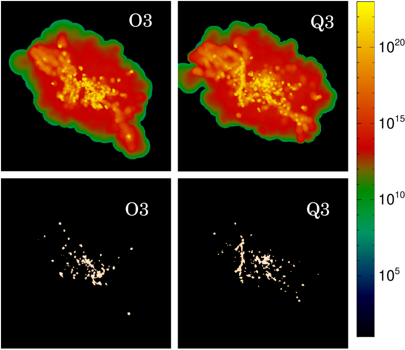
Figure 1: Comparison of ${N_{\rm HI}}$ [cm^-2] (top two panels and the range of values shown on the side with the color gradient) and DLA (bottom two panels) distribution in a dark matter halo of a mass $M_{h}\sim 1.7\times 10^{12}\,h^{-1}{M_{\odot}}$ at $z=3$ for the O3 (no wind) and Q3 (strong wind) run. Each postage stamp is about comoving $400h^{-1}{\rm\,kpc}$ (physical $\sim 100h^{-1}{\rm\,kpc}$) on a side. The DLA cross section in the O3 run is slightly larger than that of the Q3 run.

Figure 1 compares the distribution of ${N_{\rm HI}}$ and DLAs in a dark matter halo with a mass $M_{h}\sim 1.7\times 10^{12}\,h^{-1}{M_{\odot}}$ at $z=3$ for the O3 (no wind, $\chi=0.0$) run and Q3 (strong wind, $\chi=1.0$) runs. The DLA cross section of this halo is slightly higher in the O3 run than the Q3 run. The DLA columns are more concentrated near the center for the O3 run than the Q3 run, because without the wind the neutral gas is able to cool and sink deeper into the potential well. In the Q3 run, the DLA columns are distributed more broadly than the O3 run. In particular in the western side of the halo, there is a filamentary structure of DLA columns arising from overlapping DLA clouds. These DLA clouds may originate from the gas ejected by the wind but later cooled due to high gas density within the halo.

When a gas particle goes into the wind mode, our numerical wind scheme turns off its hydrodynamic interactions for a brief period of time to allow the particle to escape from the dense star-forming region. This is done in order to obtain a well-controlled mass-flux in the wind, which we picture to emanate from the surface of the star-forming region. Without the decoupling, the mass-loading would be boosted when the accelerated wind particle kicks and entrains other particles in the star-forming gas. The brief decoupling is controlled by two internal numerical parameters that limit how long the hydrodynamic forces are ignored. The primary parameter $\zeta_{\rm decoup}=\rho/\rho_{\rm th}$ determines the density $\rho$ in units of the threshold density $\rho_{\rm th}$ for star formation that the escaping wind particle needs to reach before it is allowed to interact normally again. The idea of letting the wind blow from the surface of the ISM is therefore described by the condition $\zeta_{\rm decoup}\leq 1$. A secondary numerical parameter $\ell_{\rm maxtravel}$ is introduced in order to limit the maximum time $t^{\rm max}_{\rm decoup}=\ell_{\rm maxtravel}/v_{w}$ a wind particle may stay decoupled. This length scale was just added as a precaution against the unlikely – but in case of weak winds perhaps possible – event that a wind particle ‘gets stuck’ in the ISM, i.e. cannot climb out of the gravitational potential well far enough to reach the density $\zeta_{\rm decoup}\,\rho_{\rm th}$. We stress that our expectation is that the outcome of our simulations is rather insensitive to the detailed choices for these two parameters, something that we have also confirmed in simulations of isolated galaxies when developing the model. However, in order to test whether this is also the case in our much less well resolved cosmological simulations, we have also ran four test simulations with identical initial conditions as the original Q3 run but with different values of these two internal wind parameters, as summarized in Table 2. In particular, we have varied $\zeta_{\rm decoup}$ by two orders of magnitude around our default choice of $0.1$, and we changed $\ell_{\rm maxtravel}$ between 4 and 100$\,h^{-1}{\rm kpc}$ around our default choice of $20\,h^{-1}{\rm kpc}$.

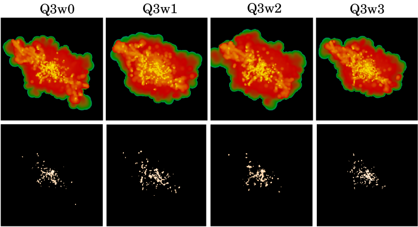
Figure 2: Distributions of ${N_{\rm HI}}$ (top row) and DLAs (bottom row) for the same dark matter halo as in Fig. 1 in the four test runs with the same color scale. Each postage stamp is about comoving $400h^{-1}{\rm\,kpc}$ (physical $\sim 100h^{-1}{\rm\,kpc}$) on a side.

The panels in Figure 2 show the Hi  column density distribution and the DLA distribution for the same halo as in Fig. 1 in the four test runs. The overall distribution of gas is similar between the different runs, but the exact locations of DLAs in each halo are not identical as a result of the changes in the decoupling prescription. Some of the difference is presumably introduced by the randomness involved in the ejection of the gas particles themselves, so that statistical comparisons between the results of the different simulations are warranted.

We hence examine the DLA cross section as a function of halo mass to see whether the distribution of DLAs is statistically different or not. Nagamine et al. (2004b) quantified the relationship between the total DLA cross section $\sigma_{\rm DLA}^{\rm co}$ (in units of comoving $h^{-2}$ kpc²; note that Fig. $2-4$ of Nagamine et al. (2004b) plotted comoving $h_{70}^{-2}\,{\rm kpc}^{2}$) and the dark matter halo mass (in units of $\,h^{-1}{M_{\odot}}$) at $z=3$ as

$$\log\,\sigma_{\rm DLA}^{\rm co}=\alpha\,(\log\,M_{\rm halo}-12)+\beta,$$ (3)

with slopes $\alpha=0.72,0.79,0.84,0.93,1.02$ and the normalization $\beta=3.94,3.99,3.98,4.03,4.18$ for the O3, P3, Q3, Q4, and Q5 runs. The slope $\alpha$ is always positive, and the massive halos have larger DLA cross section, but they are more scarce compared to less massive halos. The quantity $\beta$ gives the value of $\log\sigma_{\rm DLA}^{\rm co}$ at $M_{\rm halo}=10^{12}\,h^{-1}{M_{\odot}}$. Two qualitative trends were noted: (1) As the strength of galactic wind feedback increases (from O3 to Q3 run), the slope $\alpha$ becomes steeper while the normalization $\beta$ remains roughly constant. This is because a stronger wind reduces the gas in low-mass halos at a higher rate by ejecting the gas out of the potential well of the halo. (2) As the numerical resolution is improved (from Q3 to Q5 run), both the slope and the normalization increase. This is because with higher resolution, star formation in low-mass halos can be described better and as a result the neutral gas content is decreased due to winds. On the other hand, a lower resolution run misses the early generation of halos and the neutral gas in them.

Figure 3 shows the distribution of DLA cross section as a function of dark matter halo mass for the four test runs with different decoupling parameters. Open triangles are the median in each halo mass bin. The solid line is the power-law fit to these median points (see Table 3), and the dashed line is the fit to the original Q3 run. The shaded contours in the background give the actual distribution of halos equally spaced in logarithmic scale. Table 3 shows that the distributions of DLA cross sections in the four test runs are rather similar to that of the original Q3 run. There is a slight tendency that the slope is shallower in the four test runs than in the original Q3 run, something that could be related to extensive changes in the time integration and force calculation scheme of the simulation code relative to the older code version used in the original Q3 run, rather than to systematics introduced by the decoupling scheme. In any case, the fluctuations in our results introduced by drastic variations of the internal numerical parameters used in the decoupling scheme are much less than the large differences between the Q3 (strong wind) and O3 runs (no wind), meaning that the decoupling parameters are not a significant source of uncertainty in our results.

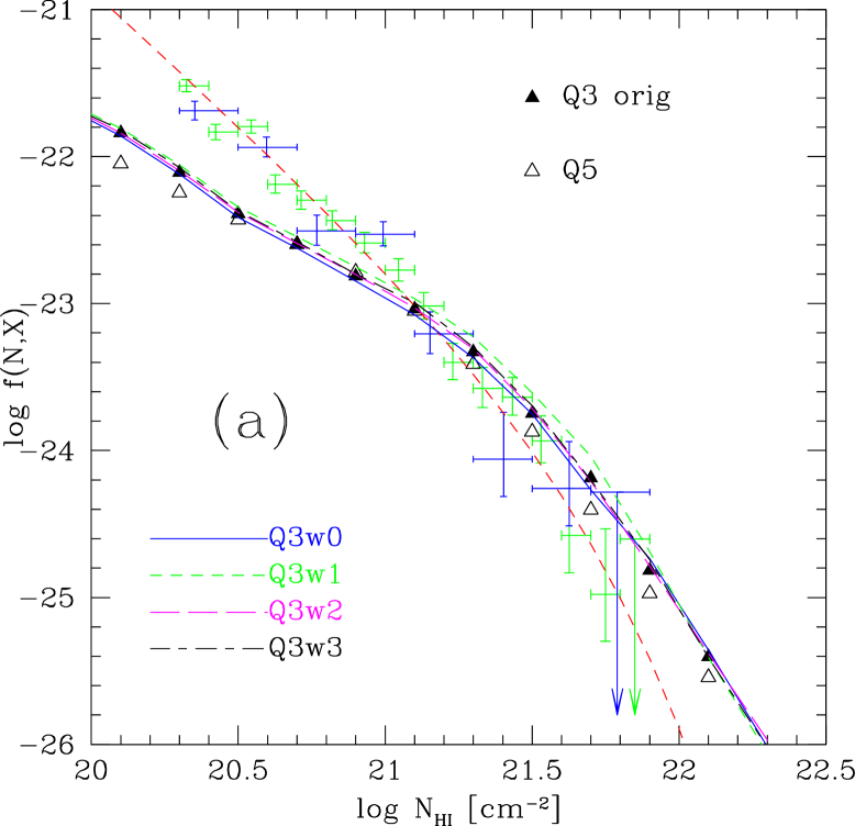
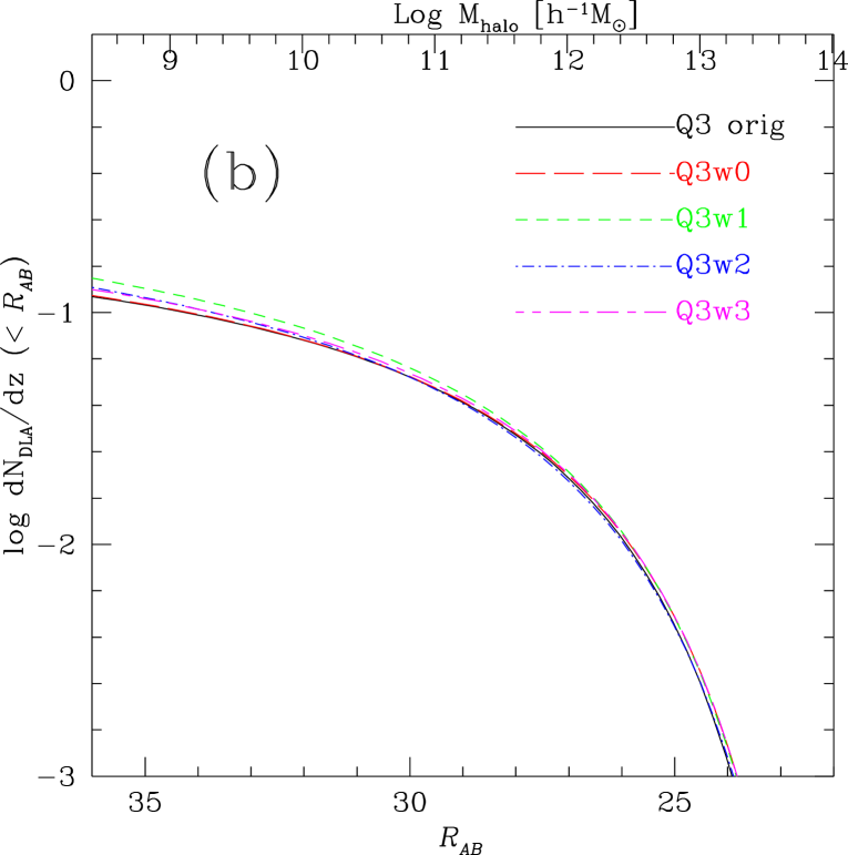
Figure 4: Panel (a): Hi  column density distribution function at $z=3$ for the four test runs with different wind parameters. The data points and the red short-dashed line are from Prochaska et al. (2005). The solid and open triangle is the results from the original Q3 and Q5 runs. Panel (b): Cumulative rate-of-incidence as a function of ${\cal R}_{AB}$ magnitude for the test runs and the original Q3 run. The results of the test runs are not so different from the original Q3 run.

Figure 4 shows the Hi  column density distribution function and the cumulative rate-of-incidence for the four test runs (see Nagamine et al., 2004b, for the definition of these two quantities). These figures also show that the statistical distribution of DLAs in the four test runs is similar to the original Q3 run. Likewise, the impact parameter distribution which we will discuss in Section 6 is also very similar to the original Q3 run for the four test runs. Therefore we focus on the original O3, P3, Q3, and Q5 runs in the following sections.

3 Differential distribution of rate-of-incidence as a function of halo mass

The differential distribution function of DLA incidence can be computed as

$$\frac{{\rm d}N_{\rm DLA}}{{\rm d}z\,{\rm d}\log M}=\frac{{\rm d}r}{{\rm d}z}[\,M\,n(M,z)\,\ln(10)\,]\,\sigma_{\rm DLA}^{\rm co}(M,z),$$ (4)

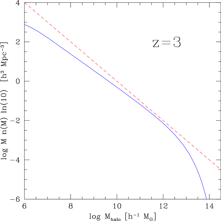
Figure 5: Dark matter halo mass function of Sheth & Tormen (1999) at $z=3$, shown in the form of $M\cdot n(M)$ to ease the interpretation of Equation (4). The red dashed line shows a power-law $n(M)\propto M^{-2}$. We use the transfer function of Eisenstein & Hu (1999) and the power spectrum is normalized to $\sigma_{8}=0.9$.

where $n(M,z)$ is the dark matter halo mass function, and ${\rm d}r/{\rm d}z=c/H(z)$ with $H(z)=H_{0}E(z)=H_{0}\sqrt{\Omega_{\rm m}(1+z)^{3}+\Omega_{\Lam}}$ for a flat universe. We use the Sheth & Tormen (1999) parameterization for $n(M)$ as shown in Figure 5. Note that the dependence on the Hubble constant disappears on the right-hand-side of Equation (4) because ${\rm d}r/{\rm d}z$ scales as $h^{-1}$, $M\,n(M)$ scales as $h^{3}$, and $\sigma_{\rm DLA}$ scales as $h^{-2}$ in the simulation. For the cumulative version of this calculation, see Equation (8) and Figure 5 of Nagamine et al. (2004b). Equation (4) can be derived from the following expression for the DLA area covering fraction on the sky along the line element $c\,{\rm d}t$:

$${\rm d}N_{\rm DLA} = n_{\rm phys}(M)\,{\rm d}M\cdot\sigma_{\rm DLA}^{\rm phys}\,\cdot c\,{\rm d}t$$ (5)

$$= (1+z)^{3}\,n_{\rm co}(M)\,dM\cdot\sigma_{\rm DLA}^{\rm phys}\cdot a\,{\rm d}r$$ (6)

$$= n_{\rm co}(M)\,dM\cdot\sigma_{\rm DLA}^{\rm co}\cdot{\rm d}r,$$ (7)

where we have used $c\,{\rm d}t=a\,{\rm d}r$ and $\sigma_{\rm DLA}^{\rm co}=(1+z)^{2}\,\sigma_{\rm DLA}^{\rm phys}$. Here $a$ is the scale factor, ${\rm d}r$ is the line element in comoving coordinate, and $n_{\rm co}(M)\,{\rm d}M$ and $n_{\rm phys}(M)\,{\rm d}M$ are the comoving and physical number density of halos in the mass range [$M$, $M+{\rm d}M$], respectively. Sometimes the ‘absorption distance’ ${\rm d}X$ is defined as ${\rm d}X\equiv\frac{H_{0}}{c}\,(1+z)^{3}\,c\,{\rm d}t=\frac{H_{0}}{c}\,(1+z)^{2}\,{\rm d}r=\frac{H_{0}}{H(z)}\,(1+z)^{2}\,{\rm d}z=(1+z)^{2}\,{\rm d}z/E(z)$, and is used to express the rate-of-incidence as

$$\frac{{\rm d}N_{\rm DLA}}{{\rm d}X}=\frac{c}{H_{0}}\,n_{\rm co}(M)\,{\rm d}M\cdot\sigma_{\rm DLA}^{\rm phys}.$$ (8)

For $z=3$ and our adopted cosmology, ${\rm d}X/{\rm d}z=3.5867$. In Equations (5) to (8), we left in the dependence on halo masses explicitly, but in practice an integral over a certain range of halo mass has to be performed when comparing with actual observations.

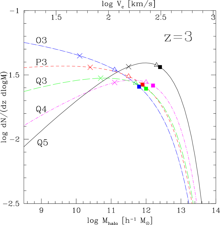
Figure 6: Differential distribution of DLA rate-of-incidence $dN/(dz\,d\log M)$ at $z=3$ as a function of halo mass, computed using Equations (3) and (4). The open crosses indicate the median halo masses $M_{50}$, and the open triangles indicate the 75 percentile of the distribution $M_{75}$. The filled squares indicate the mean DLA halo masses $\langle M_{\rm DLA}\rangle$. The top axis also indicates the circular velocity as computed by Equation (17). The differences in the shape of the distribution arise from the differences in the relationships between DLA cross section and halo mass as given by Equation (3).

We now use the power-law fits for $\sigma_{\rm DLA}^{\rm co}(M,z)$ described above to compute the differential distribution of DLA incidence via Equation (4). The result is shown in Figure 6 for all the simulations at $z=3$. The qualitative features of the curves are easy to understand. Because $n(M)\propto M^{-2}$ at $M\approx 10^{8}-10^{12}\,h^{-1}{M_{\odot}}$ (see Figure 5), the distribution is flat when $\sigma_{\rm DLA}\propto M$. In fact, $n(M)$ is slightly shallower than $M^{-2}$ (more like $M^{-1.8}$), therefore the distribution for the P3 run is almost flat at $10^{8}<M<10^{12}\,h^{-1}{M_{\odot}}$, because $\sigma_{\rm DLA}\propto M^{0.79}$ in this simulation. At masses higher than $10^{12}\,h^{-1}{M_{\odot}}$, the mass function deviates from the $M^{-2}$ power-law significantly, and the distributions for all runs quickly drop off to a small value.

The halo masses where each distribution peaks are listed in the second column of Table 4. The peak halo mass $M_{\rm peak}$ becomes larger as the feedback strength increases. For the O3 run, we indicated $M_{\rm peak}=10^{8.5}\,h^{-1}{M_{\odot}}$ in parentheses because we think that the DLA cross section rapidly falls off at this halo mass based on the work by Nagamine et al. (2004b) and the peak halo mass is simply this cutoff mass-scale. The peak halo mass is significantly larger for the Q4 ($M_{\rm peak}=10^{11.6}\,h^{-1}{M_{\odot}}$) and Q5 ($M_{\rm peak}=10^{12}\,h^{-1}{M_{\odot}}$) runs compared to other runs.

4 Mean & Median halo masses of DLAs

For each distribution shown in Figure 6, we compute the mean DLA halo mass as

$$\quad\langle M_{\rm DLA}\rangle = \frac{\int_{0}^{\infty}M\,\frac{{\rm d}N}{{\rm d}z{\rm d}\log M}{\rm d}\log M}{\int_{0}^{\infty}\frac{{\rm d}N}{{\rm d}z{\rm d}\log M}{\rm d}\log M}$$ (9)

$$= \frac{\int_{0}^{\infty}M^{2}\,n(M)~{}\sigma_{\rm DLA}(M)~{}{\rm d}\log M}{\int_{0}^{\infty}M\,n(M)~{}\sigma_{\rm DLA}(M)~{}{\rm d}\log M},$$ (10)

and the result is summarized in Table 4. The mean halo mass is smaller for the ‘no-wind’ (O3) run, and is larger for the ‘strong-wind’ (Q3 to Q5) runs. This is because of the steepening of the relationship between $\sigma_{\rm DLA}$ and $M_{\rm halo}$ as the feedback strength increases. But the mean halo mass is in the range $M_{\rm DLA}=10^{11.5}-10^{12.5}\,h^{-1}{M_{\odot}}$ for all runs. While this mass-scale is not as large as a Milky Way sized halo ($M_{\rm halo}\simeq 10^{12}-10^{13}M_{\odot}$), it is certainly more massive than that of dwarf galaxies. We also list the mean of $\log M_{\rm DLA}$ for comparison with the results by Bouche et al. (2005). We will discuss the implications of these mass-scales in Section 8.

One can also look at the median halo mass $M_{50}$, below (or above) which 50 percent of the DLA incidence is covered. The quantity $M_{50}$ is defined by the following equation:

$$0.5=\int_{M_{50}}^{\infty}n(M)~{}\sigma_{\rm DLA}(M)~{}{\rm d}M~{}/~{}\int_{0}^{\infty}n(M)~{}\sigma_{\rm DLA}(M)~{}{\rm d}M.$$ (11)

The median halo mass is always smaller than $\langle M_{\rm DLA}\rangle$ for all runs. The values of $M_{50}$ are indicated by the open crosses in Figure 6, and $\langle M_{\rm DLA}\rangle$ are indicated by the filled squares. We emphasize that $M_{50}$ is much smaller than $\langle M_{\rm DLA}\rangle$, and that $\langle M_{\rm DLA}\rangle$ could be biased towards a large value because of the weighting by the halo mass.

Furthermore, in Table 4 we also give the 75 percentile halo mass $M_{75}$, below which 75 percent of the DLA incidence is covered. For example, in the Q5 run, halos with masses $M_{\rm halo}<10^{12.3}\,h^{-1}{M_{\odot}}$ are responsible for 75% of the DLA incidence at $z=3$. The values of $M_{75}$ are shown with open triangles in Figure 6.

5 Luminosity distribution of DLA galaxies

The luminosity distribution of DLA galaxies constrains their nature, facilitating the interpretation of observations of DLA galaxies. Nagamine et al. (2004e) computed the spectra of galaxies in the same simulations used in this paper using the population synthesis model of Bruzual & Charlot (2003, hereafter BClib03) based on the stellar mass, formation time, and metallicity of each stellar particle that makes up simulated galaxies. Using the computed spectra, we sum up the monochromatic luminosity at rest-frame 1655Å  (chosen because it corresponds to the observed-frame ${\cal R}$ band of the $U_{n}G{\cal R}$ system) of all the galaxies enclosed in the maximum radius of each dark matter halo identified by the friends-of-friends grouping algorithm (Davis et al., 1985). The following formula (see Eq.(2) of Night et al., 2006) is used to compute the absolute AB magnitude at 1655Å, because BClib03 outputs its spectrum $L_{\lambda}$ in units of $L_{\odot}$ Å^-1 where $L_{\odot}=3.826\times 10^{33}$ erg s^-1:

$$M_{AB}=-2.5\log(\lambda^{2}L_{\lambda})+13.83.$$ (12)

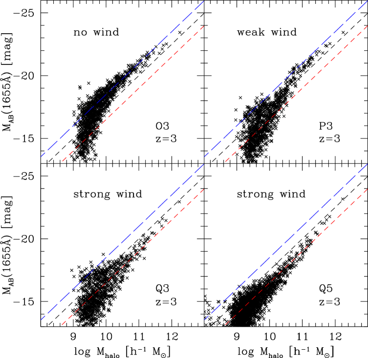
Figure 7: Halo mass vs. absolute AB magnitude at 1655Å  at $z=3$. See text for the description of the three dashed lines.

Figure 7 shows the relationship between $M_{AB}$ and the halo mass for O3, P3, Q3, and Q5 runs at $z=3$. The three dashed lines correspond to

$$M_{AB}=-2.5\,(\log M_{\rm halo}-12)-C_{1},$$ (13)

where $C_{1}=23.5,22.5$, and 21.5 from top to bottom, and $M_{\rm halo}$ is in units of $\,h^{-1}{M_{\odot}}$. We adopt $C_{1}=23.5$ for the O3 run, $C_{1}=22.5$ for the P3 run, and $C_{1}=21.5$ for the Q3 and Q5 runs. This figure shows that, on average, the galaxies in the ‘no-wind’ run (O3) are brighter than those in the ‘strong-wind’ run (Q3 & Q5) by about a factor of six. This was pointed out in Figure 6 of Nagamine et al. (2004e) and was attributed to the suppression of star formation by a strong galactic wind.

Here, the apparent and absolute magnitudes are related to each other as

$$m_{AB}=M_{AB}+2.5\,\log(1+z)+5\,\log(d_{L}/10{\rm pc}),$$ (14)

where $d_{L}$ is the luminosity distance. Notice the positive sign in front of the 2nd term (which is normally negative); this is because of the definition of $M_{AB}$ in Equation (12) (see also Equation (2) of Night et al., 2006). Inserting Equation (13) into Equation (14) and using $d_{L}(z=3)=2.542\times 10^{4}\,h_{70}^{-1}\,{\rm Mpc}$ for our flat $\Lam$ cosmology, we obtain the relation between the apparent magnitude ${\cal R}_{AB}$ and the halo mass $M_{\rm halo}$ as

$${\cal R}_{AB}=-2.5\,\log M_{\rm halo}+C_{2}-5\log h_{70},$$ (15)

where $C_{2}=55.03$ (O3 run), 56.03 (P3 run), and 57.03 (Q3 and Q5 run), and $M_{\rm halo}$ is in units of $\,h^{-1}{M_{\odot}}$. These numerical values are consistent with the ones adopted by Haehnelt et al. (2000), where they assumed $m_{AB}=26.6-7.5\log(v_{c}/200\,\rm km\,s^{-1})=-2.5\,\log M_{\rm halo}+55.7$ for a flat $\Lam$ cosmology. The circular velocity $v_{c}$ at a radius of overdensity 200 is computed as

$$v_{c} \equiv \left(\frac{GM_{\rm halo}}{R_{200}}\right)^{1/2}=\left[GM_{\rm halo}^{2/3}\left(\frac{4\pi}{3}\bar{\rho}\,200\right)^{1/3}\right]^{1/2}$$ (16)

$$= 123.5\,\left(\frac{M_{\rm halo}}{10^{11}\,h^{-1}{M_{\odot}}}\right)^{1/3}\left(\frac{1+z}{4}\right)^{1/2}\,\rm km\,s^{-1}$$ (17)

for our flat $\Lam$ cosmology and $\bar{\rho}$ is the mean density of the universe at redshift $z$.

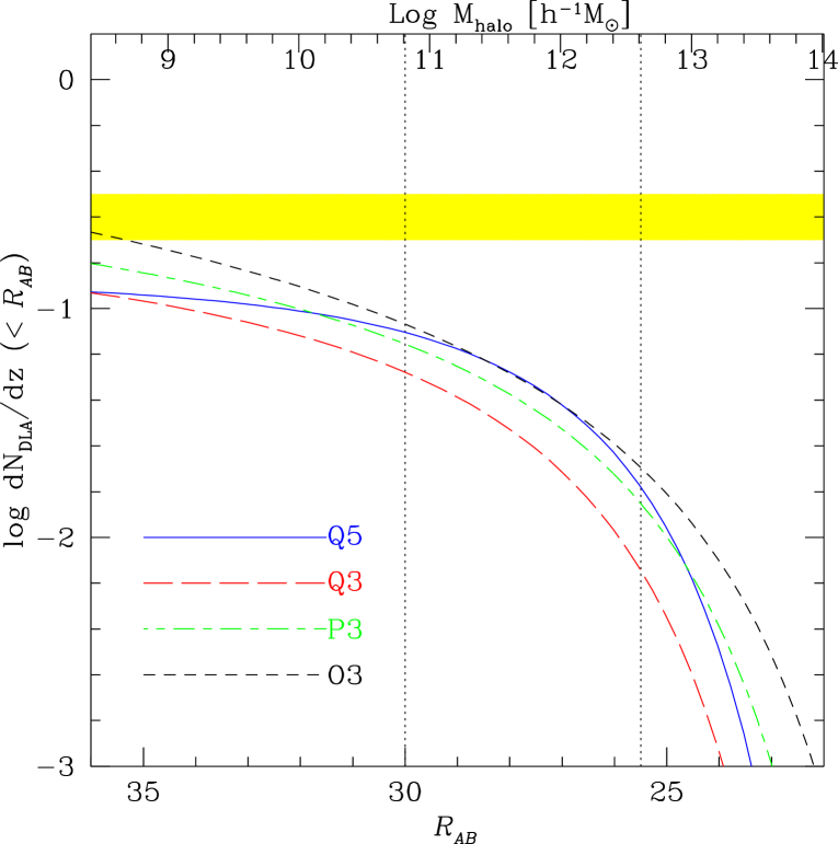
Figure 8: Cumulative distribution function of DLA rate-of-incidence as a function of apparent ${\cal R}_{AB}$ magnitude. The spectroscopic limit ${\cal R}_{AB}=25.5$ and the limiting magnitude ${\cal R}_{AB}=30$ are indicated by the vertical dotted lines. The top axis gives the corresponding halo masses using the relationship for the Q3 and Q5 runs; ${\cal R}_{AB}=-2.5\log M_{\rm halo}+57.03-5\log h_{70}$ (Eq. [15]). The yellow band is the observational estimate by Prochaska et al. (2005, see text for details).

Figure 8 shows the cumulative distribution for the absolute value of DLA rate-of-incidence as a function of apparent ${\cal R}_{AB}$ magnitude of host galaxies. The slight differences in these results from Fig. 5 of Nagamine et al. (2004b) are due to an improved calculation of the halo mass function with a more accurate integration of the power spectrum when computing the mass variance $\sigma(M)$. The yellow hatched region shows the observational estimate $\log({\rm d}N/{\rm d}z)=-0.60\pm 0.10$ at $z=3$ obtained from Fig. 8 of Prochaska et al. (2005). We estimate that the range of ${\rm d}N/{\rm d}X$ centered at $z=3$ is [$0.065,0.09$] with a central value $0.07$, and then multiply ${\rm d}N/{\rm d}X$ by ${\rm d}X/{\rm d}z=3.587$ for $z=3$ to obtain the above observational value. We find that the P3, Q3 and Q5 runs underpredict ${\rm d}N/{\rm d}z$. We will discuss this discrepancy further in Section 8.

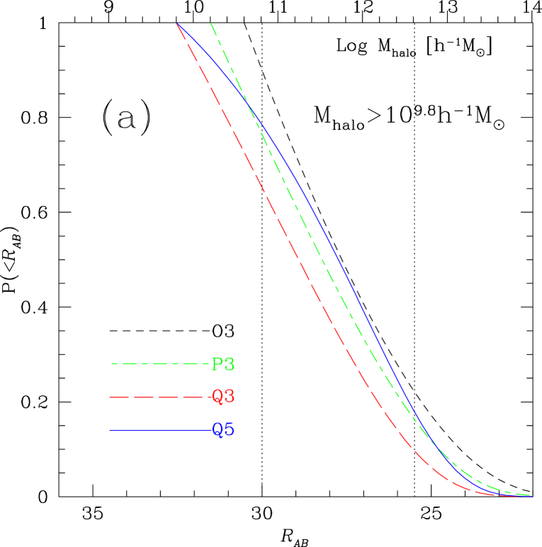
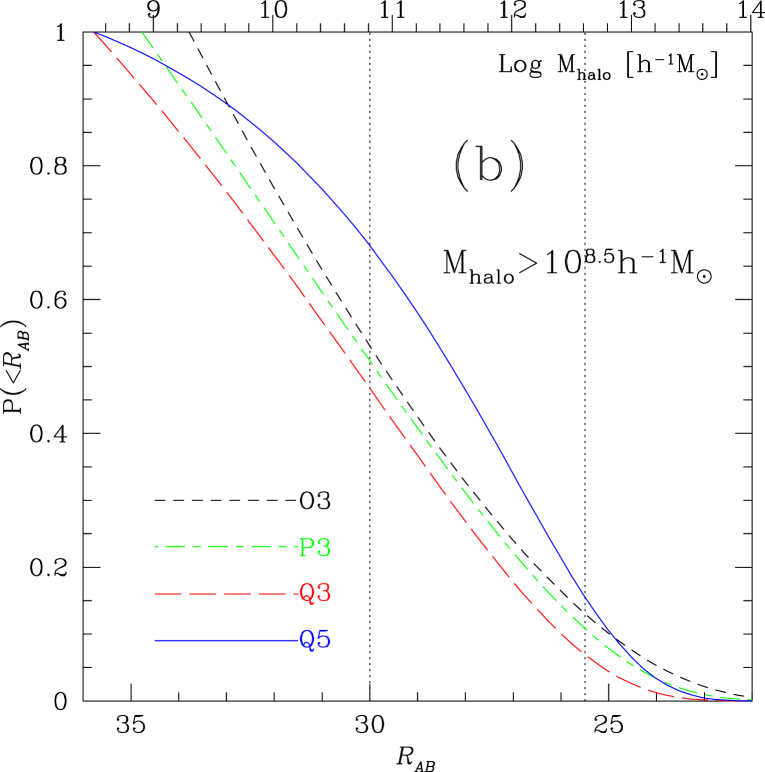
Figure 9: Cumulative probability distribution of DLA rate-of-incidence as a function of apparent ${\cal R}_{AB}$ magnitude at $z=3$. Panel (a) is when the distribution is normalized by the value at $M_{\rm halo}=10^{9.8}\,h^{-1}{M_{\odot}}$; i.e., assuming there would be no DLAs in halos less massive than this value. This roughly reproduces the result of Haehnelt et al. (2000). Panel (b) is when the distribution is normalized by the value at $M_{\rm halo}=10^{8.5}\,h^{-1}{M_{\odot}}$, which is more consistent with the results of our SPH simulations. The top axis shows the scaling with halo mass for the Q3 and Q5 runs, ${\cal R}_{AB}=-2.5\log M_{\rm halo}+57.03-5\log h_{70}$ (Eq. [15].)

It is clear from Figure 8 that only a very small fraction of DLA incidence is associated with galaxies brighter than ${\cal R}_{AB}=25.5$. This is more evident in Figure 9 where the cumulative probability distribution of DLA incidence is shown. In panel (a), we normalize the cumulative distribution by the value at $M_{\rm halo}=10^{9.8}\,h^{-1}{M_{\odot}}$, or equivalently, halos less massive than the above value are assumed not to host DLAs at all. Here we roughly reproduce the result of Haehnelt et al. (2000) where they adopted the cutoff circular velocity of $50\,\rm km\,s^{-1}$, which corresponds to $M_{\rm halo}\simeq 10^{9.8}\,h^{-1}{M_{\odot}}$. Similarly to their result, we find that for this cutoff mass, only $10-20$% of DLA sight-lines are contributed by galaxies brighter than the spectroscopic limit ${\cal R}_{AB}=25.5$, and $70-90$% of the DLA sight-lines are contributed by galaxies brighter than magnitude ${\cal R}_{AB}=30$.

However, according to the work by Nagamine et al. (2004b), only halos with masses $M_{\rm halo}\gtrsim 10^{8.5}\,h^{-1}{M_{\odot}}$ (or equivalently $v_{c}>18\,\rm km\,s^{-1}$) contribute to the DLA cross section (see their Figure 2 & 3), so the cutoff velocity of $50\,\rm km\,s^{-1}$ adopted by Haehnelt et al. (2000) might be too high. In Figure 9b we show a case with cutoff halo mass $M_{\rm halo}>10^{8.5}\,h^{-1}{M_{\odot}}$. Here, less than 15% of DLAs are contributed by galaxies with ${\cal R}_{AB}<25.5$, and $50-70$% by those with ${\cal R}_{AB}<30$.

6 Impact parameter distribution

We also compute the impact parameter distribution (i.e., projected separation between DLA sight-lines and the nearest galaxy) using our simulations. Nagamine et al. (2004b, c) calculated the neutral hydrogen column density ${N_{\rm HI}}$ for each pixel with a size of $\epsilon^{2}$ on projected planes covering the face of each dark matter halo, where $\epsilon$ is the smoothing length of the simulation. The pixels with ${N_{\rm HI}}>2\times 10^{20}$ cm^-2 were equally regarded as DLA sight-lines. Therefore there are multiple DLA sight-lines per halo. Galaxies in our simulations are identified as collections of star particles. Nagamine et al. (2004e, d) computed the spectrophotometric properties of simulated galaxies based on the formation time, stellar mass, and metallicity of individual star particles, and showed that the simulated luminosity functions agree reasonably well with the observations if a mean extinction of $E(B-V)=0.15$ is assumed. This level of extinction is consistent with observationally derived values for the Lyman break galaxies (LBGs) at $z\sim 3$ (Shapley et al., 2001).

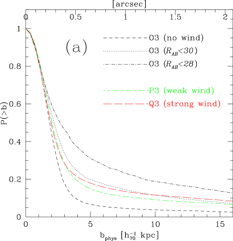
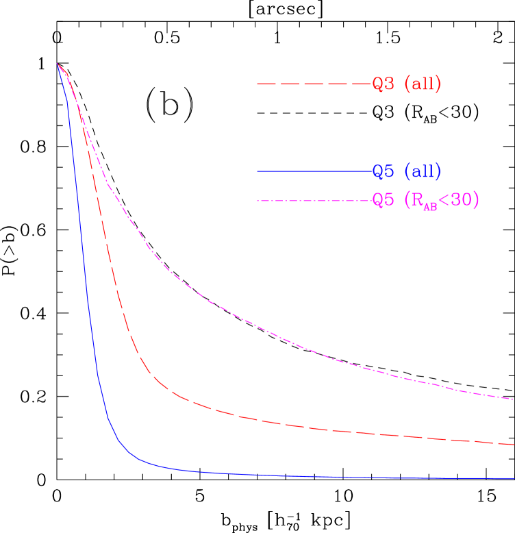
Figure 10: Cumulative probability distribution of DLA rate-of-incidence as a function of projected impact parameter $d_{\rm phys}$ in units of physical $h_{70}^{-1}\,{\rm kpc}$ and angular scale in units of arc second at $z=3$. Panel (a) shows the results of O3 (no wind), P3 (weak wind), and Q3 (strong wind) runs. Panel (b) shows the results of Q3 and Q5 runs. In both panels, we also show the results when the search for the nearest galaxy is limited to those brighter than a certain ${\cal R}_{AB}$ magnitude.

Knowing the locations of both DLAs and galaxies in the simulation, we compute the impact parameter for each DLA pixel by searching for the nearest galaxy on the projected plane. If a nearby galaxy cannot be found within the same halo, we allow the search to extend further. Figure 10 shows the cumulative probability distribution of DLA incidence as a function of impact parameter $b_{\rm phys}$ (in units of physical $h_{70}^{-1}\,{\rm kpc}$). Figure 10a shows the results of the O3, P3, and Q3 runs to highlight the impact of galactic wind feedback. As the feedback strength increases, gas in low mass halos is ejected more efficiently, and the neutral hydrogen content decreases. Therefore, the relative contribution from higher mass halos increases and the impact parameter distribution becomes broader. Another notable feature of this plot is that, if all galaxies are allowed to be a candidate DLA galaxy no matter how faint they are, then the majority (over 90% for the O3 run, and 80% for the P3 and Q3 runs) of DLA sight-lines have the nearest galaxy within $b_{\rm phys}=5$ $h_{70}^{-1}\,{\rm kpc}$. However, if we limit the search for the nearest galaxy to those brighter than ${\cal R}_{AB}=30$ or 28 mag, then a large fraction of DLAs, in particular those in low mass halos, cannot be associated with a qualified galaxy within the same halo, resulting in a much broader impact parameter distribution. About 30% of all DLA sight-lines in the O3 run have impact parameters $b_{\rm phys}>5$ $h_{70}^{-1}\,{\rm kpc}$ for the limited search of a nearest galaxy with ${\cal R}_{AB}<28$.

Figure 10b shows the result of the Q3 and Q5 runs. The higher resolution run (Q5) has a narrower impact parameter distribution than the lower resolution run (Q3), because it can resolve more low-mass galaxies which host DLAs with low impact parameters. Therefore the relative contribution from DLAs with low impact parameters becomes larger. Also, galaxies in massive halos will be better resolved in the Q5 run than in the Q3 run, and this will also result in smaller impact parameters for the DLAs in massive halos. We expect that, in a run with even higher resolution, the impact parameter distribution will remain as narrow as that of the Q5 run, because increasing the resolution always seems to increase the relative number of columns with low impact parameters. We also show the case where we limit the search for the nearest galaxy to those brighter than ${\cal R}_{AB}=30$ mag. In this case, results from the Q3 and Q5 runs agree well, and about 40% of all DLA sight-lines have impact parameters $b_{\rm phys}>5$ $h_{70}^{-1}\,{\rm kpc}$.

For most of the DLAs with low impact parameters, there is a galaxy within the same dark matter halo. However, for a few to 10% of the DLA sight-lines that are in the low mass halos in O3, P3, and Q3 runs, there are no galaxies within the same halo and the nearest galaxy is in another halo, as indicated by the offset of the curves at the bottom right corner of the plot in panel (a). In the Q5 run, there are almost no DLA sight-lines that do not have a galaxy within the same halo, and the distribution approaches zero at large $b_{\rm phys}$ values in panel (b).

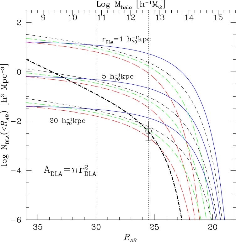
Figure 11: Cumulative, comoving number density of DLAs as a function of apparent ${\cal R}_{AB}$ magnitude for 3 different values of assumed DLA physical radius $r_{\rm DLA}=1\,h_{70}^{-1}\,{\rm kpc}$, 5 $h_{70}^{-1}\,{\rm kpc}$, and 20 $h_{70}^{-1}\,{\rm kpc}$. The area of each DLA is $A_{\rm DLA}=\pi r_{\rm DLA}^{2}$. For each value of $r_{\rm DLA}$, four different lines are shown: Q5 run (blue solid line), O3 (black dashed), P3 (green short-dash long-dash), and Q3 (red long-dashed). The thick black dot-dashed line is the cumulative comoving number density of LBGs obtained by integrating the observed luminosity function by Adelberger & Steidel (2000). The data point at ${\cal R}_{AB}=25.5$ shows the comoving number density of LBGs $N_{\rm LBG}=4\times 10^{-3}h^{-3}\,{\rm Mpc}^{-3}$.

Overall, our impact parameter distribution seems to be much narrower than that obtained by Haehnelt et al. (2000) if we do not limit our search to the bright galaxies. Figure 3 of Haehnelt et al. (2000) suggests that 60% of DLA sight-lines have $b<1$ arc second, but our results indicate that more than 80% of DLAs have $b<1$ arc second if we do not limit our search for the nearest galaxy to those with ${\cal R}_{AB}<30$ mag. The differences between the two results might stem from subhalos within the massive halos in the simulations, which Haehnelt et al. (2000) did not take into account. The calculation of Haehnelt et al. (2000) assigns a single effective DLA radius to each halo and assumes that the DLAs cover a circular area centered on each halo, whereas in our simulations, massive halos contain numerous galaxies and the geometry of the DLA cross section cannot be characterized by a circular area centered on each halo. For example, the most massive halo in the O3 run contains 143 galaxies, and in the Q5 run 1110 galaxies. Therefore the DLAs in the simulation would be able to find the nearest galaxy at distances much smaller than the effective DLA radius computed by Haehnelt et al. (2000). But when we limit our search for the nearest galaxy to those with ${\cal R}_{AB}<30$ mag, then our results for the Q3 and Q5 run become similar to that obtained by Haehnelt et al. (2000). It is not very clear how our results compare to Figure 11d by Mo et al. (1998), as these authors examined only the differential distribution of impact parameter and not the cumulative probability distribution. But their differential distribution peaks at 2.5 $h^{-1}$ kpc and a significant fraction (more than 50%) of the area under the curve appears to come from $b<5\,h^{-1}$ kpc, in reasonable agreement with our results.

7 Number density of DLAs

Finally, we discuss the comoving number density of DLAs. Assuming that the characteristic covering area of each DLA $A_{\rm DLA}$ is fixed with a physical radius $r_{\rm DLA}$ (i.e., $A_{\rm DLA}=\pi\,r_{\rm DLA}^{2}$), we can compute the cumulative number density of DLAs as a function of halo mass as

$$N_{\rm DLA}(>M)=\int_{M}^{\infty}{\rm d}M\,n(M)\,\frac{\sigma_{\rm DLA}^{\rm phys}}{A_{\rm DLA}},$$ (18)

where the definitions of $n(M)$ and $\sigma_{\rm DLA}^{\rm phys}$ are the same as described in Section 3. Note again that $\sigma_{\rm DLA}$ is the total DLA cross section of each dark matter halo; in other words, if there are 100 DLA gas clouds in a massive halo, then this halo has a total DLA cross section of $\sigma_{\rm DLA}^{\rm phys}=100\,A_{\rm DLA}$. Then, using Equation (13) allows us to obtain the cumulative comoving number density of DLAs as a function of apparent ${\cal R}_{AB}$ magnitude $N_{\rm DLA}(<{\cal R}_{AB})$ as shown in Figure 11. Here, three different values of physical radius for DLAs are assumed: $r_{\rm DLA}=1,5$ and $20\,h_{70}^{-1}\,{\rm kpc}$. For each radius, the results of four simulations (O3, P3, Q3, and Q5 runs) are shown. Also given is the cumulative number density of LBGs, $N_{\rm LBG}(<m)$, computed by integrating the Schechter luminosity function of Adelberger & Steidel (2000) with parameters $(m^{*},\alpha,\Phi^{*}[h^{3}{\rm Mpc}^{-3}])=(24.54,-1.57,4.4\times 10^{-3})$:

$$N_{\rm LBG}(<m)=\int_{m}^{0}\Phi(m){\rm d}m,$$ (19)

where $\Phi(m)=(0.4\,\ln 10)\,\Phi^{*}\,10^{\mu\,(\alpha+1)}\,\exp(-10^{\mu})$ as a function of apparent magnitude $m$, and $\mu=0.4\,(m^{*}-m)$. The comoving number density of LBGs at $z=3$, $N_{\rm LBG}=4\times 10^{-3}$ (Adelberger et al., 2003), is also shown as the data point at the magnitude limit of ${\cal R}_{AB}=25.5$.

Figure 11 shows that the comoving number density of DLAs is larger than that of LBGs down to the magnitude limit of ${\cal R}_{AB}=25.5$ if the physical radius of each DLA is smaller than $r_{\rm DLA}\simeq 5\,h_{70}^{-1}\,{\rm kpc}$. The two number densities roughly agree with each other at ${\cal R}_{AB}=25.5$ when $r_{\rm DLA}\simeq 20\,h_{70}^{-1}\,{\rm kpc}$. Earlier, Schaye (2001) argued that the observed DLA rate-of-incidence can be accounted for if each LBG were accompanied by a DLA cross section of $\pi r^{2}=\pi(19h^{-1}{\rm\,kpc})^{2}$ assuming $({\rm d}N/{\rm d}z)_{\rm DLA}=0.20$ and $N_{\rm LBG}=0.016\,h^{3}\,{\rm Mpc}^{-3}$ (down to ${\cal R}_{AB}=27$ mag). His result is in good agreement with the result of the Q5 run with $r_{\rm DLA}=20\,h_{70}^{-1}\,{\rm kpc}$ shown in Figure 11. However, this large DLA radius is somewhat unrealistic because this model implies that all halos with masses $M_{\rm halo}\gtrsim 10^{12}\,h^{-1}{M_{\odot}}$ host such a large disk at $z=3$ that are responsible for DLAs, and none of the less massive halos host DLAs at all. This picture is quite the contrary to our simulation results that indicate halos down to masses $M_{\rm halo}=10^{8.5}\,h^{-1}{M_{\odot}}$ could host DLAs, and simulated DLAs in lower mass halos are clumpy and smaller in cross section.

The existence of extended disks at high redshift can be observationally tested by searching for extended emission from stars in deep imaging data such as the Hubble Deep Fields (Bouwens et al., 2003; Ferguson et al., 2004). The most recent study on this issue by Bouwens et al. (2004) using the Hubble Ultra Deep Field (HUDF) suggests that high redshift $UBVi$-dropout galaxies are compact in size ($\sim 0.1-0.3$ arc seconds) and that extended sources ($\gtrsim 0.4$ arc sec, $\gtrsim 3\,{\rm kpc}$) are rare. Another observational analysis of high redshift galaxies in HUDF by Wolfe & Chen (2006) also suggests that there are no extended disks down to very faint surface brightness. Our simulation results and impact parameter distribution are in accord with these observational results. If our picture is realistic and each DLA has a physical size of $\lesssim 5\,{\rm kpc}$, then it means that there are multiple clumps of DLAs around massive galaxies such as LBGs at $z\sim 3$, although the fraction of DLA incidence covered by the DLAs in massive halos ($M_{\rm halo}\gtrsim 10^{12}\,h^{-1}{M_{\odot}}$) is smaller than that in less massive halos that host very faint galaxies (${\cal R}_{AB}\gtrsim 27$ mag).

8 Discussion & Conclusions

Using state-of-the-art cosmological SPH simulations, we performed a numerical study of a galactic wind model, and examined the distribution of DLA rate-of-incidence as a function of halo mass, galaxy apparent magnitude, and impact parameter. We find that the majority of DLA rate-of-incidence in the simulations is dominated by relatively lower mass halos ($M_{\rm halo}<10^{12}\,h^{-1}{M_{\odot}}$) and faint (${\cal R}_{AB}>25.5$) galaxies. This conclusion agrees with the generic prediction of the semi-analytic model of Kauffmann (1996), that the DLA galaxies at high redshift will typically be smaller, more compact, and less luminous than disk galaxies at the present epoch, although this analysis was restricted to an $\Omega_{\rm m}=1$ universe. More recent work by Okoshi & Nagashima (2005) also suggests that the low-redshift ($z\leq 1$) DLA galaxies are mainly low-luminosity, compact galaxies. Combined with our results, the dominance of faint galaxies in DLA incidence seems to be a generic prediction of a CDM model. This can be ascribed to the steeply rising dark matter halo mass function towards lower masses in CDM models, and to the fact that the small DLA cross sections in these low mass halos add up to a large portion of the total DLA incidence when multiplied by a large number of low-mass halos.

8.1 On the DLA Halo Mass

We characterize the differential distribution of DLA rate-of-incidence $dN/(dz\,d\log M)$ with various halo masses listed in Table 4. We find that the mean DLA halo mass increases with increasing galactic wind feedback strength, because winds are able to eject the gas in lower mass halos, suppressing their DLA cross section, resulting in a larger relative contribution from higher mass halos (see also Nagamine et al., 2004b). The mean DLA halo mass for the Q5 run was found to be $\langle M_{\rm DLA}\rangle=10^{12.4}\,h^{-1}{M_{\odot}}$ and $\langle\log M_{\rm DLA}[\,h^{-1}{M_{\odot}}]\rangle=11.3$ when we limit the DLA distribution to $M_{\rm halo}>10^{8.5}\,h^{-1}{M_{\odot}}$. The latter value is close to that obtained by Bouche et al. (2005, $\langle\log M_{\rm DLA}[\,h^{-1}{M_{\odot}}]\rangle=10.9$), but this comparison is not fully appropriate because their simulation only resolved halos with masses $\log(M_{\rm halo}[\,h^{-1}{M_{\odot}}])>10.5$ and they did not attempt to extrapolate their halo distribution using an analytic halo mass function. Therefore, the value of mean DLA halo mass they derived was biased toward a larger value owing to limited resolution, and it is an upper limit as the authors described in their paper. Since their simulation did not include galactic wind feedback, their result should be compared to that of our O3 (‘no-wind’) run. In fact, the value of concern for the O3 run is $\langle\log M_{\rm DLA}[\,h^{-1}{M_{\odot}}]\rangle=10.4$, and it is lower than their halo mass resolution when we take the full distribution of DLAs into account down to $M_{\rm halo}=10^{8.5}\,h^{-1}{M_{\odot}}$ We also note that there are large differences between $\langle\log M_{\rm DLA}\rangle$, $\log\langle M_{\rm DLA}\rangle$, & $M_{50}$, therefore the former two quantities are not to be confused with $M_{50}$.

Given that the results of the Q3 and Q5 runs do not agree, the results given here may appear as if they have not converged yet. According to the results of the R-Series presented by Nagamine et al. (2004b), we consider that the lowest halo mass that could host DLAs is $M_{\rm halo}\sim 10^{8.5}\,h^{-1}{M_{\odot}}$. In the Q5 run, there are 150 dark matter particles for a halo of this mass, therefore it is close to the resolution limit. The Q5 run should be close to the convergence if not fully converged. It is possible that in a run with higher resolution run than the Q5 run, the mean DLA halo mass could be even higher than that of the Q5 run.

There have already been several observational attempts to constrain DLA halo masses via cross-correlation between DLAs and LBGs (Gawiser et al., 2001; Adelberger et al., 2003; Bouche & Lowenthal, 2003, 2004), but owing to limited sample sizes, the results have been mostly inconclusive. More recently, Cooke et al. (2006) has measured the cross-correlation between 11 DLAs and 211 LBGs, and constrained the DLA halo mass to be $\approx 10^{11.2}M_{\odot}$. It is encouraging that this measurement is close to our results listed in Table 4. The result of Cooke et al. (2006) suggests that at least some DLAs are associated with relatively massive halos, close to the LBG halo masses ($\sim 10^{12}M_{\odot}$). There could of course be some distribution in the LBG halo masses (perhaps from $M_{\rm halo}=10^{10}$ to $10^{13}M_{\odot}$; see the broad distribution of stellar masses at the magnitude limit ${\cal R}_{AB}=25.5$ in Figure 4 of Nagamine et al. (2004e)), and likewise DLAs could also have a broad halo mass distribution. The majority of DLA sight-lines in the simulations are dominated by lower mass halos in spite of a relatively large mean DLA halo mass, which is also reflected in the large differences between the median halo mass and the mean halo mass as we summarize in Table 4.

8.2 On the Luminosity Distribution

As for the luminosity distribution of DLA galaxies, we find that only about 10% of DLA sight-lines are associated with galaxies brighter than ${\cal R}_{AB}=25.5$ mag. This suggests that only about 10% of DLA galaxies will be found in searches for the bright LBGs at $z\sim 3$ down to ${\cal R}_{AB}=25.5$. The dominance of DLA sight-lines by the faint galaxies is a generic result in all of our simulations, therefore we consider that this conclusion will not change in a higher resolution run than the Q5 run.

We reproduce the result of Haehnelt et al. (2000) when we cut off the DLA distribution at $M_{\rm halo}=10^{9.8}\,h^{-1}{M_{\odot}}$ (or equivalently a circular velocity of $v_{c}=50\,\,\rm km\,s^{-1}$), and in this case $70-90$% of DLA sight-lines are associated with galaxies brighter than ${\cal R}_{AB}=30$ mag. This agreement with the Haehnelt et al. result is not surprising, because they assumed a relation $\sigma_{\rm DLA}\propto v_{c}^{\alpha}\propto M_{\rm halo}^{\alpha/3}$ with $\alpha\sim 2.5-3$ and a normalization matched to the observed $dN/dz$ of DLAs, and our SPH simulations suggest $\alpha=2.2-3.1$ depending on the feedback strength and resolution. However, our simulations indicate that even lower mass halos contribute to the DLA cross section, and when we cut off our DLA distribution at $M_{\rm halo}=10^{8.5}\,h^{-1}{M_{\odot}}$, only $50-70$% of DLAs are associated with galaxies brighter than ${\cal R}_{AB}=30$ mag. Thus, it would be possible to detect DLA galaxies with $\sim 50$% efficiency by searching down to ${\cal R}_{AB}=30$ mag.

While the dominance of faint galaxies among DLAs seems to be a generic prediction of the CDM model, we note that the recent photometric survey of low-redshift ($z<1$) DLA galaxies by Chen & Lanzetta (2003) on the contrary suggests that a large contribution from dwarf galaxies is not necessary to account for their observed DLA incidence. However, this conclusion might be affected by the ‘masking effect’ emphasized by Okoshi & Nagashima (2005). Current DLA surveys might be biased against the detection of DLAs associated with faint and compact galaxies, because such galaxies would be buried under the bright QSO that has to be masked for the detection of a DLA galaxy. This effect would be more severe if the impact parameters are small as our present work suggests, as well as some observational studies of high redshift DLA galaxies that imply very small impact parameters less than several kpc (i.e., $\lesssim 1$ arcsec) (Fynbo et al., 1999; Kulkarni et al., 2000; Møller et al., 2002, 2004). Fynbo et al. (1999) suggests that, based on the properties of a limited sample of observed high redshift candidate DLA galaxies, a large fraction ($\sim 70$%) of DLA galaxies at $z\simeq 3$ could be fainter than ${\cal R}_{AB}=28$ mag. It is possible that evolution with redshift is relatively strong as suggested by the chemical evolution model of Lanfranchi & Friaca̧ (2003), in the sense that the high redshift DLAs are dominated by dwarf galaxies and the low-redshift ones by disks. But the latter scenario seems to be inconsistent with the predictions by Okoshi & Nagashima (2005).

Hopkins et al. (2005) also argued for the dominance of faint galaxies for the DLA galaxies based on the comparison of global quantities such as the density of gas mass, stellar mass, metal mass, and star formation rate. They also suggested that the DLAs may be a distinct population from LBGs, but we note that the dominance of faint galaxies for the DLA rate-of-incidence does not immediately mean that DLAs do not exist in LBGs. It simply means that the area covered by the DLAs associated with LBGs is much smaller than that in faint galaxies. We plan to investigate the connection between DLAs and LBGs in more detail in future work.

8.3 On the Impact Parameter Distribution

Our distribution of impact parameters is significantly narrower than that of Haehnelt et al. (2000), and we ascribe this difference to substructures within the massive halos in our simulations. The differential distribution of Mo et al. (1998, Figure 11d) seems to be in better agreement with our results, with roughly half of DLAs having $b_{\rm phys}<3h^{-1}{\rm\,kpc}$, but this comparison is probably not fully appropriate because their model is restricted to centrifugally supported disks. Indeed, Haehnelt et al. (2000) comment that their effective DLA radius is about a factor of 10 larger than the expected scale length of a centrifugally supported disk if the angular momentum of the gas owes to tidal torquing during the collapse of a dark matter halo. However, we caution that the large effective DLA radius for a massive halo does not necessarily mean that DLAs consist of only large disks centered on halos; i.e., the DLA cross section could be distributed to hundreds of galaxies (associated with subhalos) embedded in a massive halo, with each DLA gas cloud being fairly compact. This point was also emphasized by Gardner et al. (2001, Section 4.1).

Our narrow impact parameter distribution at first sight might seem inconsistent with that of Gardner et al. (2001), but in fact they are not. Gardner et al. (2001) mostly used SPH simulations with 64³ particles which were able to resolve halos only down to $M_{\rm halo}=8.2\times 10^{10}M_{\odot}$, and found that nearly all DLAs lie within $15-20$ kpc of a galaxy center. Given their mass resolution, they were not able to simulate galaxies fainter than ${\cal R}_{AB}\simeq 30$ mag at $z=3$. If we limit the search for the nearest galaxy to those brighter than ${\cal R}_{AB}=30$ mag (see Figure 10b), our simulations suggest that 80% of DLAs are within $b_{\rm phys}=15\,h_{70}^{-1}\,{\rm kpc}$, which is consistent with the results of Gardner et al. (2001). However if we include the fainter galaxies that were not resolved in the simulations by Gardner et al. (2001), then the overall impact parameter distribution becomes narrow, with more than 80% of DLA sight-lines having $b_{\rm phys}<5\,h_{70}^{-1}\,{\rm kpc}$.

The small impact parameters suggest that DLAs in our simulations are compact, and this has significant implications for the nature of DLAs. The compactness of the simulated DLAs can also be observed in the projected distribution of DLAs in Figure 2 & 3 of Nagamine et al. (2004c). There, one can see that the DLAs are at the centers of galaxies and coincide with star-forming regions quite well, covering roughly half the area of the star-forming region. These results are at odds with the idea that DLAs mainly originate from gas in large galactic disks (e.g., Wolfe et al., 1986; Turnshek et al., 1989; Prochaska & Wolfe, 1997, 1998). The overall agreement between the simulations and observations found by Nagamine et al. (2004b, c) was encouraging, but the simulations with galactic wind feedback now seem to underpredict the DLA rate-of-incidence (see Figure 8) compared to the new observational estimate by Prochaska et al. (2005) utilizing the SDSS Data Release 3. This is because our simulations underpredict the column density distribution $f({N_{\rm HI}})$ at $20<\log{N_{\rm HI}}<21$ by a factor of $2-3$ even in our highest resolution run with a smoothing length of comoving 1.23 $h^{-1}{\rm\,kpc}$. Cen et al. (2003) reported that they did not have this problem, but instead they significantly overpredicted $f({N_{\rm HI}})$ at $\log{N_{\rm HI}}>22$ as well as $\Omega_{\rm gas}$, and had to introduce dust extinction to match observations. The inconsistency in $f({N_{\rm HI}})$ between SPH simulations and observations and the compactness of the simulated DLAs might be related to the well-known angular momentum problem (Robertson et al., 2004, and references therein) in hydrodynamic simulations, where simulated disk galaxies are known to be too small and centrally concentrated. This is a problem that is not easy to solve, and future studies are needed using both Eulerian mesh simulations and SPH simulations. In summary, there persist tensions between the predicted and observed $f({N_{\rm HI}})$, large observed velocity widths (which favors large and thick disks), and the predicted compactness of DLAs (cf. Jedamzik & Prochaska, 1998).

8.4 On the Resolution Effects and Numerical Convergence

Finally let us discuss the resolution and convergence issues of the present work. In Figures 6 and 8 for example, the results of the Q3 and Q5 run do not seem to have converged. This does not mean that our models for star formation and feedback are ill-defined. In fact, Springel & Hernquist (2003a) and Springel & Hernquist (2003b) showed that the code and the simulations converge well in runs with star formation and wind feedback. The reason for the non-convergence seen in Figures 6 and 8 can be primarily ascribed to the restricted dynamic range of current cosmological simulations, which is present in almost all modern numerical work.

In cosmological simulations, the issue of establishing numerical convergence is clouded by the fact that an increase of the resolution always modifies the problem one solves – one suddenly sees a whole new generation of low-mass galaxies that weren’t there previously. This effect disappears only once the simulations resolve all halos capable of cooling, and it was achieved by the ‘R-series’ in the earlier work by Nagamine et al. (2004b), in which we deduced our lower limit for the DLA halo mass. When lower mass halos are newly resolved in the Q5 run which were not present in the Q3 run, it steepens the slope of the relation between DLA cross-section and halo mass, reducing the relative contribution by the low-mass halos to the total DLA incidence. This change causes the difference between the results of Q3 and Q5 run in Figures 6 and 8, and it can be regarded as a cautionary sign for the effect of resolution on these calculations. In the Q5 run, there are 150 dark matter particles for a halo with $M_{\rm halo}=10^{8.5}\,h^{-1}{M_{\odot}}$, so the results of the Q5 run should be close to the convergence if not fully converged.

Note however that we nevertheless find it highly useful to explore the consequences and predictions of our particular wind feedback model for DLAs, even if the present work eventually can only be used to demonstrate the failure of the model. The model is numerically well posed, and therefore allows various predictions on the properties on DLAs and galaxies to be made (Nagamine et al., 2004b, c, 2005, e, d, a, 2005b, 2005a). We are thus able to determine where our numerical model agrees and disagrees with the observational data on DLAs and galaxies. It is exactly such a comparison that makes DLA observations so useful for theory, because they can teach us in this way about galaxy formation. In the future when the computers become fast enough to achieve full dynamic range of mass and spatial scales without employing a series of simulations, we will be able to better address the issues of numerical resolution and convergence.

Table 1: Simulations

Run	${N_{\rm p}}$	$m_{\rm DM}$	$m_{\rm gas}$	$\epsilon$	wind
O3	$144^{3}$	$2.42\times 10^{7}$	$3.72\times 10^{6}$	2.78	none
P3	$144^{3}$	$2.42\times 10^{7}$	$3.72\times 10^{6}$	2.78	weak
Q3	$144^{3}$	$2.42\times 10^{7}$	$3.72\times 10^{6}$	2.78	strong
Q4	$216^{3}$	$7.16\times 10^{6}$	$1.10\times 10^{6}$	1.85	strong
Q5	$324^{3}$	$2.12\times 10^{6}$	$3.26\times 10^{5}$	1.23	strong

Note. — Simulations employed in this study. All simulations have a comoving box size of 10 $h^{-1}{\rm\,Mpc}$. The (initial) number of gas particles $N_{\rm P}$ is equal to the number of dark matter particles, so the total particle count is twice ${N_{\rm p}}$. $m_{\rm DM}$ and $m_{\rm gas}$ are the masses of dark matter and gas particles in units of $\,h^{-1}{M_{\odot}}$, respectively, and $\epsilon$ is the comoving gravitational softening length in units of $h^{-1}{\rm\,kpc}$, The value of $\epsilon$ is a measure of spatial resolution.

Table 2: Test runs with different wind parameters

Run	$\zeta_{\rm decoup}$	$\ell_{\rm maxtravel}\,[h^{-1}{\rm\,kpc}]$
Q3	0.1	20	default values
Q3w0	1.0	20	higher $\rho_{\rm decoup}$
Q3w1	0.01	20	lower $\rho_{\rm decoup}$
Q3w2	0.1	4	shorter $t^{\rm max}_{\rm decoup}$
Q3w3	0.1	100	longer $t^{\rm max}_{\rm decoup}$

Note. — The density $\rho_{\rm decoup}=\zeta_{\rm decoup}\,\rho_{\rm th}$ denotes the threshold density for the decoupling of the hydrodynamic force, and $t^{\rm max}_{\rm decoup}=\ell_{\rm maxtravel}/v_{w}$ parameterize the maximum allowed time of the decoupling.

Table 3: Fit parameters for test runs

Run	slope $\alpha$	normalization $\beta$
Q3	0.84	3.98
Q3w0	0.83	3.96
Q3w1	0.80	3.99
Q3w2	0.80	3.95
Q3w3	0.82	3.97

Note. — Fit parameters to the DLA area vs. halo mass relationship.

Table 4: DLA halo masses

Run	$\log M_{\rm peak}$	$\log M_{50}$	$\log M_{75}$	$\log\langle M_{\rm DLA}\rangle$	$\langle\log M_{\rm DLA}\rangle$
O3	(8.5)	10.1	11.1	11.8	10.4
P3	9.6	10.4	11.5	11.9	10.6
Q3	10.8	10.7	11.7	12.0	10.8
Q4	11.6	11.1	12.0	12.2	11.1
Q5	12.0	11.5	12.3	12.4	11.3

Note. — Various DLA halo masses in units of $\,h^{-1}{M_{\odot}}$ that characterize the differential distribution $dN/(dz\,d\log M$) with the distribution cutoff at $M_{\rm halo}=10^{8.5}\,h^{-1}{M_{\odot}}$. The following quantities are listed: peak halo mass $M_{\rm peak}$, median halo mass $M_{50}$ (i.e., 50 percentile of the distribution), 75 percentile of the distribution $M_{75}$, mean halo mass $\langle M_{\rm DLA}\rangle$ (Equation (10)), and the mean of $\log M_{\rm halo}$ rather than $M_{\rm halo}$ itself for the comparison with the result by Bouche et al. (2005). The peak halo mass for O3 run is shown in the parenthesis because it is the cutoff mass itself of the distribution.

Figure 3: DLA cross section vs. halo mass at $z=3$ for the four test runs with different wind parameters. Open triangles are the median in each halo mass bin. The red solid line is the power-law fit to these median points (Table 3), and the black dashed line is the fit to the original Q3 run. The shaded contour in the background is the actual distribution of halos equally spaced in logarithmic scale.

References

- Adelberger & Steidel (2000) Adelberger, K. L. & Steidel, C. C. 2000, ApJ, 544, 218
- Adelberger et al. (2003) Adelberger, K. L., Steidel, C. C., Shapley, A. E., & Pettini, M. 2003, ApJ, 584, 45
- Bouche et al. (2005) Bouche, N., Gardner, J. P., Weinberg, D. H., Davé, R., & Lowenthal, J. D. 2005, ApJ, 628, 89
- Bouche & Lowenthal (2003) Bouche, N. & Lowenthal, J. D. 2003, ApJ, 596, 810
- Bouche & Lowenthal (2004) —. 2004, ApJ, 609, 513
- Bouwens et al. (2004) Bouwens, R. J., Blakeslee, J. P., Illingworth, G. D., Broadhurst, T. J., & Franx, M. 2004, ApJ, 611, L1
- Bouwens et al. (2003) Bouwens, R. J., Broadhurst, T. J., & Illingworth, G. D. 2003, ApJ, 593, 640
- Bruzual & Charlot (2003) Bruzual, G. & Charlot, S. 2003, MNRAS, 344, 1000
- Cen et al. (2005) Cen, R., Nagamine, K., & Ostriker, J. P. 2005, ApJ, 635, 86
- Cen et al. (2003) Cen, R., Ostriker, J. P., Prochaska, J. X., & Wolfe, A. M. 2003, ApJ, 598, 741
- Chen & Lanzetta (2003) Chen, H.-W. & Lanzetta, K. M. 2003, ApJ, 597, 706
- Cooke et al. (2006) Cooke, J., Wolfe, A. M., Gawiser, E., & Prochaska, J. X. 2006, ApJ, 636, L9
- Davé et al. (1999) Davé, R., Hernquist, L., Katz, N., & Weinberg, D. H. 1999, ApJ, 511, 521
- Davis et al. (1985) Davis, M., Efstathiou, G., Frenk, C. S., & White, S. D. M. 1985, ApJ, 292, 371
- Eisenstein & Hu (1999) Eisenstein, D. & Hu, P. 1999, ApJ, 511, 5
- Ferguson et al. (2004) Ferguson, H. C., Dickinson, M., Giavalisco, M., Kretchmer, C., Ravindranath, S., Idzi, R., Taylor, E., Conselice, C. J., et al. 2004, ApJ, 600, L107
- Fynbo et al. (1999) Fynbo, J. U., Møller, P., & Warren, S. J. 1999, MNRAS, 305, 849
- Gardner et al. (1997a) Gardner, J., Katz, N., Hernquist, L., & Weinberg, D. H. 1997a, ApJ, 484, 31
- Gardner et al. (2001) —. 2001, ApJ, 559, 131
- Gardner et al. (1997b) Gardner, J., Katz, N., Weinberg, D. H., & Hernquist, L. 1997b, ApJ, 486, 42
- Gawiser et al. (2001) Gawiser, E., Wolfe, A. M., Prochaska, J. X., Lanzetta, K. M., Yahata, N., & Quirrenbach, A. 2001, ApJ, 562, 628
- Haardt & Madau (1996) Haardt, F. & Madau, P. 1996, ApJ, 461, 20
- Haehnelt et al. (1998) Haehnelt, M., Steinmetz, M., & Rauch, M. 1998, ApJ, 495, 647
- Haehnelt et al. (2000) —. 2000, ApJ, 534, 594
- Hopkins et al. (2005) Hopkins, A. M., Rao, S. M., & Turnshek, D. A. 2005, ApJ, 630, 108
- Jedamzik & Prochaska (1998) Jedamzik, K. & Prochaska, J. X. 1998, MNRAS, 296, 430
- Katz et al. (1996a) Katz, N., Weinberg, D. H., & Hernquist, L. 1996a, ApJS, 105, 19
- Katz et al. (1996b) Katz, N., Weinberg, D. H., Hernquist, L., & Miralda-Escudé, J. 1996b, ApJ, 457, L57
- Kauffmann (1996) Kauffmann, G. 1996, MNRAS, 281, 475
- Kulkarni et al. (2000) Kulkarni, V. P., Hill, J. M., Schneider, G., Weymann, R. J., Storrie-Lombardi, L. J., Rieke, M., Thompson, R. I., & Jannuzi, B. T. 2000, ApJ, 536, 36
- Kulkarni et al. (2001) —. 2001, ApJ, 551, 37
- Lanfranchi & Friaca̧ (2003) Lanfranchi, G. A. & Friaca̧, A. C. S. 2003, MNRAS, 343, 481
- Lanzetta et al. (1995) Lanzetta, K. M., Wolfe, A. M., & Turnshek, D. A. 1995, ApJ, 440, 435
- Le Brun et al. (1997) Le Brun, V., Bergeron, J., Boissé, P., & Deharveng, J. M. 1997, A&A, 321, 733
- Maller et al. (2001) Maller, A., Prochaska, J. X., Somerville, R. S., & Primack, J. 2001, ApJ, 326, 1475
- McCarthy et al. (1987) McCarthy, P. J., van Breugel, W., & Heckman, T. 1987, AJ, 93, 264
- Mo et al. (1998) Mo, H. J., Mao, S., & White, S. D. M. 1998, MNRAS, 295, 319
- Møller et al. (2004) Møller, P., Fynbo, J. U., & Fall, S. M. 2004, A&A, 422, L33
- Møller et al. (2002) Møller, P., Warren, S. J., Fall, S. M., Fynbo, J. U., & Jakobsen, P. 2002, ApJ, 574, 51
- Nagamine et al. (2004a) Nagamine, K., Cen, R., Hernquist, L., Ostriker, J. P., & Springel, V. 2004a, ApJ, 610, 45
- Nagamine et al. (2005a) —. 2005a, ApJ, 627, 608
- Nagamine et al. (2005b) —. 2005b, ApJ, 618, 23
- Nagamine et al. (2004b) Nagamine, K., Springel, V., & Hernquist, L. 2004b, MNRAS, 348, 421
- Nagamine et al. (2004c) —. 2004c, MNRAS, 348, 435
- Nagamine et al. (2005) Nagamine, K., Springel, V., & Hernquist, L. 2005, in IAU Symposium, ed. M. Colless, L. Staveley-Smith, & R. A. Stathakis, 266
- Nagamine et al. (2004d) Nagamine, K., Springel, V., Hernquist, L., & Machacek, M. 2004d, MNRAS, 355, 638
- Nagamine et al. (2004e) —. 2004e, MNRAS, 350, 385
- Night et al. (2006) Night, C., Nagamine, K., Springel, V., & Hernquist, L. 2006, MNRAS, 366, 705
- Okoshi & Nagashima (2005) Okoshi, K. & Nagashima, M. 2005, ApJ, 623, 99
- Okoshi et al. (2004) Okoshi, K., Nagashima, M., Gouda, N., & Yoshioka, S. 2004, ApJ, 603, 12
- Péroux et al. (2003) Péroux, C., McMahon, R. G., Storrie-Lombardi, L. J., & Irwin, M. J. 2003, MNRAS, 346, 1103
- Pettini et al. (2001) Pettini, M., Shapley, A. E., Steidel, C. C., Cuby, J.-G., Dickinson, M., Moorwood, A. F. M., Adelberger, K. L., & Giavalisco, M. 2001, ApJ, 554, 981
- Prochaska et al. (2005) Prochaska, J. X., Herbert-Fort, S., & Wolfe, A. M. 2005, ApJ, 635, 123
- Prochaska & Wolfe (1997) Prochaska, J. X. & Wolfe, A. M. 1997, ApJ, 487, 73
- Prochaska & Wolfe (1998) —. 1998, ApJ, 507, 113
- Prochaska & Wolfe (2002) —. 2002, ApJ, 566, 68
- Prochaska et al. (2001) Prochaska, J. X., Wolfe, A. M., Tytler, D., Burles, S., et al. 2001, ApJS, 137, 21
- Rao & Turnshek (2000) Rao, S. M. & Turnshek, D. A. 2000, ApJS, 130, 1
- Robertson et al. (2004) Robertson, B. E., Yoshida, N., Springel, V., & Hernquist, L. 2004, ApJ, 606, 32
- Schaye (2001) Schaye, J. 2001, ApJ, 559, L1
- Shapley et al. (2001) Shapley, A. E., Steidel, C. C., Adelberger, K. L., Dickinson, M., Giavalisco, M., & Pettini, M. 2001, ApJ, 562, 95
- Sheth & Tormen (1999) Sheth, R. K. & Tormen, G. 1999, MNRAS, 308, 119
- Springel (2005) Springel, V. 2005, MNRAS, 364, 1105
- Springel & Hernquist (2002) Springel, V. & Hernquist, L. 2002, MNRAS, 333, 649
- Springel & Hernquist (2003a) —. 2003a, MNRAS, 339, 289
- Springel & Hernquist (2003b) —. 2003b, MNRAS, 339, 312
- Storrie-Lombardi & Wolfe (2000) Storrie-Lombardi, L. J. & Wolfe, A. M. 2000, ApJ, 543, 552
- Theuns et al. (2002) Theuns, T., Viel, M., Kay, S., Schaye, J., Carswell, R. F., & Tzanavaris, P. 2002, ApJ, 578, L5
- Turnshek et al. (1989) Turnshek, D. A., Wolfe, A. M., Lanzetta, K. M., Briggs, F. H., Cohen, R. D., Foltz, C. B., Smith, H. E., & Wilkes, B. J. 1989, ApJ, 344, 567
- Weatherley et al. (2005) Weatherley, S. J., Warren, S. J., Möller, P., Fall, S. M., Fynbo, J. U., & Croom, S. M. 2005, MNRAS, 358, 985
- Wolfe & Chen (2006) Wolfe, A. M. & Chen, H.-W. 2006, ApJ, 652, 981
- Wolfe et al. (1995) Wolfe, A. M., Lanzetta, K. M., & Foltz, C. B. 1995, ApJ, 454, 698
- Wolfe et al. (1986) Wolfe, A. M., Turnshek, D. A., Smith, H. E., & Cohen, R. D. 1986, ApJS, 61, 249