HYADES OXYGEN ABUNDANCES FROM THE $\lambda 6300$ [O I] LINE: THE GIANT-DWARF OXYGEN DISCREPANCY REVISITED

Abstract

We present the results of our abundance analysis of Fe, Ni, and O in high S/N, high-resolution VLT/UVES and McDonald/2dcoudé spectra of nine dwarfs and three giants in the Hyades open cluster. The difference in Fe abundances derived from Fe II and Fe I lines ([Fe II/H] – [Fe I/H]) and Ni I abundances derived from moderately high-excitation ($\chi\approx 4.20\;\mathrm{eV}$) lines are found to increase with decreasing $T_{\rm eff}\;$for the dwarfs. Both of these findings are in concordance with previous results of over-excitation/ionization in cool young dwarfs. Oxygen abundances are derived from the $\lambda 6300$ [O I] line, with careful attention given to the Ni I blend. The dwarf O abundances are in star-to-star agreement within uncertainties, but the abundances of the three coolest dwarfs ($4573\leq T_{\mathrm{eff}}\leq 4834\;\mathrm{K}$) evince an increase with decreasing $T_{\rm eff}$. Possible causes for the apparent trend are considered, including the effects of over-dissociation of O-containing molecules. O abundances are derived from the near-UV $\lambda 3167$ OH line in high-quality Keck/HIRES spectra, and no such effects are found– indeed, the OH-based abundances show an increase with decreasing $T_{\rm eff}$, leaving the nature and reality of the cool dwarf [O I]-based O trend uncertain. The mean relative O abundance of the six warmest dwarfs ($5075\leq T_{\mathrm{eff}}\leq 5978\;\mathrm{K}$) is $\mathrm{[O/H]}=+0.14\pm 0.02$, and we find a mean abundance of $\mathrm{[O/H]}=+0.08\pm 0.02$ for the giants. Thus, our updated analysis of the $\lambda 6300$ [O I] line does not confirm the Hyades giant-dwarf oxygen discrepancy initially reported by King & Hiltgen (1996), suggesting the discrepancy was a consequence of analysis-related systematic errors. LTE Oxygen abundances from the near-IR, high-excitation O I triplet are also derived for the giants, and the resulting abundances are approximately 0.28 dex higher than those derived from the [O I] line, in agreement with NLTE predictions. NLTE corrections from the literature are applied to the giant triplet abundances; the resulting mean abundance is $\mathrm{[O/H]}=+0.17\pm 0.02$, in decent concordance with the giant and dwarf [O I] abundances. Finally, Hyades giant and dwarf O abundances as derived from the $\lambda 6300$ [O I] line and high-excitation triplet, as well as dwarf O abundances derived from the near-UV $\lambda 3167$ OH line, are compared, and a mean cluster O abundance of $\mathrm{[O/H]}=+0.12\pm 0.02$ is achieved and represents the best estimate of the Hyades O abundance.

1 INTRODUCTION

Oxygen is the most abundant element in the Galaxy after H and He. The predominant nucleosynthesis site of ${}^{16}\mathrm{O}$, the most abundant O isotope ($99.8\%$ of O in the Solar System), is He burning at the cores of massive stars (Clayton, 2003). The O is subsequently dispursed into the interstellar medium (ISM) when the progenitor massive stars experience their death throes as Type II supernovae (Woosley & Weaver 1995). Thus, mapping O abundances in various Galactic environments, such as H II regions (e.g., Esteban et al. 2005), planetary nebulae (e.g., Péquignot, & Tsamis 2005), presolar grains (e.g., Nittler et al. 1997), and stars (e.g., Wheeler, Sneden, & Truran 1989; Bensby, Feltzing, & Lundström 2004), is an irreplaceable tool in tracing the chemical evolution of the Galaxy and constraining supernovae rates. Determining stellar O abundances may make the most crucial contribution to this endeavor. Significant O overabundances relative to Fe observed in metal-poor stars is seen as a direct consequence of the rapid O enrichment of the ISM in the early Galaxy, resulting from Type II supernovae, compared to the slower enrichment of Fe, which has its primary nucleosynthesis site in Type Ia supernovae (Kobayashi et al. 1998; Matteucci & Greggio 1986). A clear elucidation of the [O/Fe] versus Fe abundance trend is a critical component of understanding Galactic evolution (Wheeler et al., 1989).

Deriving stellar O abundances can also provide important tests of stellar nucleosynthesis and mixing in evolved stars (e.g., Vanture & Wallerstein 1999). Stellar evolution models make precise predictions of the variations in surface chemical compositions due to mixing of nuclear processed material from the core as stars evolve off the main sequence (MS; Boothroyd & Sackman 1999). Known as the “first dredge-up,” this mixing episode is not predicted to alter the composition of ${}^{16}\mathrm{O}\;$in the atmospheres of low-mass ($\lesssim 2.5\;\mathrm{M_{\sun}}$) stars. In the present study, we rivisit the Hyades giant-dwarf oxygen discrepancy described by King & Hiltgen (1996; henceforth KH96), who determined O abundances from the $\lambda 6300$ [O I] line for two dwarfs and three red giants in the Hyades ($625\;\pm 50\;\mathrm{Myr}$; Perryman et al. 1998) open cluster; the O abundances of the giants were found to be 0.23 dex lower than those of the dwarfs. This result was unexpected, and KH96 discussed two possible sources of the discrepancy. The first possibility is that the difference is real and due to the dredging of O-depleted material from core regions that have been mixed with ON-processed nuclei in the giants. The second possibility discussed by KH96 is that the difference is a result of systematic errors in their analysis that may be related to the ability of the $\lambda 6300$ [O I] line to deliver accurate O abundances. Either one of these scenarios, if confirmed, could potentially have a considerable effect on our understanding of the evolution of O in the Galaxy, and we explore them more fully in the next two subsections.

1.1 Hyades Giants and the First Dredge-Up

The extent of the changes in surface compositions due to the first dredge-up are dependent on both mass and metallicity (Iben, 1965), so before predictions for the Hyades giants can be compared to observations, an estimation of their masses must be obtained (the metallicity of the Hyades is well-determined, e.g. Paulson, Sneden, & Cochran 2004). There are four giants in the Hyades cluster- $\gamma\;\mathrm{Tau}$, $\delta\;\mathrm{Tau}$, $\epsilon\;\mathrm{Tau}$, and $\theta^{1}\;$ Tau- all of which apparently reside at the same location on the cluster HR diagram and are of the same evolutionary state (Perryman et al. 1998; de Bruijne, Hoogerwerf, & de Zeeuw 2001). Data from the Hipparcos astrometry satellite, along with a 631 Myr isochrone of Girardi et al. (2000), have been used to show that the Hyades giants fall on the cluster red clump (de Bruijne et al., 2001). Using data from Perryman et al. (1998), de Bruijne et al. report masses ($M/M_{\sun}$) of 2.32, 2.30, 2.32, and 2.32 for $\gamma\;\mathrm{Tau}$, $\delta\;\mathrm{Tau}$, $\epsilon\;\mathrm{Tau}$, and $\theta^{1}\;$ Tau, respectively, with a common uncertainty of 0.10. Fortuitously, $\theta^{2}\;$ Tau, a star located at the turnoff in the cluster’s HR diagram and a proper-motion companion to $\theta^{1}\;$ Tau, is a spectroscopic binary. The orbital solutions for the $\theta^{2}\;$ Tau system have been determined by Tomkin, Pan, & McCarthy (1995), who find a mass of $M/M_{\sun}=2.1\;\pm 0.3$ for the primary component. de Bruijne et al report a mass of $M/M_{\sun}=2.37\;\pm 0.10$ for the primary component of $\theta^{2}$ Tau, in good agreement with the Tomkin et al. result. Gilroy (1989) determined a similar value for the turnoff mass ($M/M_{\sun}=2.2\;\pm 0.12$) for the Hyades by fitting the cluster color-magnitude diagram (CMD) with the isochrones of Vandenberg (1985). The combined estimates of the turnoff and red clump masses present an evolutionary picture that is consistent with expectations, i.e., stars at the turnoff are slightly less massive than those that have evolved to the red giant branch (RGB). So it seems the mass estimates of $M/M_{\sun}\sim 2.3$ for the Hyades giants reported by de Bruijne et al. (2001) are plausible and are accepted here.

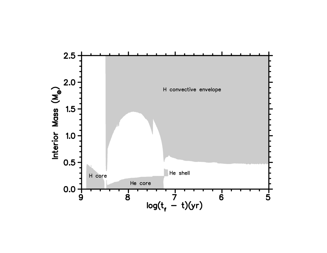
We have employed the Clemson-American University of Beirut Stellar Evolution Code to model the evolution and expected changes in the surface composition of the Hyades giants; the code is fully described in The, El Eid, & Meyer (2000). For the present study, a mass of $M/M_{\sun}=2.5$, a metallicity of $Z=0.025$ ($\mathrm{[m/H]}\approx+0.10$), the Schwarzchild criterion for convection, and a mixing length parameter, $\alpha$ ($\alpha=l/H_{\mathrm{p}}$, where $l$ is the convective scale length and $H_{\mathrm{p}}$ is the pressure scale height), of $2.0$ have been adopted. As stated above, the amount of mixing as a result of the first dredge-up depends on both the mass and metallicity of the star: the core radial zones exposed to nuclear processed material are extended outward in more massive (due to higher core temperatures) and more metal-poor (due to lower opacities) stars (Charbonnel, 1994). We thus consider using a model characterized by a mass that is slightly higher than those described above as conservative, because the model should overestimate the amount of mixing that has occurred in the Hyades giants. The adopted metallicity is characteristic of that for the Hyades, which is well-known to be metal-rich compared to the Sun (see §3.3). The model was evolved approximately 800 Myr and was stopped during He shell burning phase; the temporal scale of our model should be sufficient for the Hyades giants, which have an age of about 625 Myr. The stellar structure as a function of time is given in Figure 1; time is plotted on a logarithmic scale in terms of ($\mathrm{t}_{\mathrm{f}}-\mathrm{t}$), where $\mathrm{t}_{\mathrm{f}}\approx 7.9\times 10^{8}\;\mathrm{yr}$, the total elapsed time, and $\mathrm{t}$ is time since $\mathrm{t}=0$. Convective regions are shown as gray areas, and radiative regions are white. The core remains convective for nearly 475 Myr, during which time it contracts at a near constant rate. Afterwards, shell H burning commences, and the core becomes radiative. This continues for a short duration until the conditions in the core are sufficient so that He burning begins, and the star experiences the first dredge-up. At this time, nuclear processed material from the core is mixed with the pristine material in the atmosphere. It can be seen in Figure 1 that at no subsequent stage in the star’s evolution does the surface convection zone extend deep enough to dredge further processed material.

Changes in the surface composition of the Hyades giants predicted by our $2.5\;M_{\sun}$ model can now be compared to observations. The CNO bi-cycle is the main energy generation source for stars with masses greater than about 1.3 $M_{\sun}$, and the abundances of some of the isotopes involved with the reactions- ${}^{12}\mathrm{C}$, ${}^{13}\mathrm{C}$, and ${}^{16}\mathrm{O}$- are of interest here. The general expectation is that the abundances of ${}^{12}\mathrm{C}\;$and ${}^{16}\mathrm{O}\;$are reduced and those of ${}^{13}\mathrm{C}\;$are enhanced in the convective core as a result of the reactions comprising the bi-cycle (e.g., El Eid 1994). Changes in the abundances of these isotopes are manifested at the surface as a result of the first dredge-up. The first reaction of the bi-cycle converts ${}^{12}\mathrm{C}\;$into ${}^{13}\mathrm{C}\;$via the reaction ${}^{12}\mathrm{C}(p,\gamma)^{13}\mathrm{N}(\beta^{+}\nu)^{13}\mathrm{C}$ and is followed by the conversion of ${}^{13}\mathrm{C}\;$into ${}^{14}\mathrm{N}\;$via ${}^{13}\mathrm{C}(p,\gamma)^{14}\mathrm{N}$. The second of these reactions lags the first due to its dependence on the ${}^{13}\mathrm{C}\;$abundance; the general result is a decrease in the ${}^{12}\mathrm{C}\;$abundance and an increase in the ${}^{13}\mathrm{C}\;$and ${}^{14}\mathrm{N}\;$abundances. Indeed, the surface ${}^{12}\mathrm{C}$/${}^{13}\mathrm{C}\;$ratio as our $2.5\;M_{\sun}$ model evolves onto the MS is 90.0 and reduces to 23.6 after the first dredge-up, and as expected, the ratio remains constant following this initial reduction (Figure 2). Spectroscopic determinations of the ${}^{12}\mathrm{C}$/${}^{13}\mathrm{C}\;$ratio for the Hyades giants are available in the literature, and our theoretical value is in good concordance with the observational results. Tomkin, Luck, & Lambert (1976) found ${}^{12}\mathrm{C}$/${}^{13}\mathrm{C}\;$ratios of 19, 23, 22, and 20 for $\gamma\;\mathrm{Tau}$, $\delta\;\mathrm{Tau}$, $\epsilon\;\mathrm{Tau}$, and $\theta^{1}\;$ Tau, respectively, and Gilroy (1989) reported ratios of 26.0, 24.0, 25.5, and 27.5 for the same four stars. The reported uncertainty of the Tomkin et al. (1976) values are $\pm 15\%$, and no uncertainty is given by Gilroy. Again, these ${}^{12}\mathrm{C}$/${}^{13}\mathrm{C}\;$ratios are in good agreement with our theoretical value.

Another check of the plausibility of our model is the overall reduction of ${}^{12}\mathrm{C}\;$after the first dredge-up. The dominant isotopic species for C is ${}^{12}\mathrm{C}$, making up $98.9\%$ Solar System composition, so observationally determined C abundances are equivalent to the model ${}^{12}\mathrm{C}\;$abundance. Comparing the initial and final ${}^{12}\mathrm{C}\;$abundances from our model, a reduction by a factor of 1.56 is found. Comparison to observations is more uncertain in this case because of the lack of accurate C abundances for the Hyades dwarfs. We have thus determined C abundances for two dwarfs in our sample (see §3.4.2) and compared the mean abundance to that of the giants as reported by KH96, which is based on previous determinations. The reduction factor is approximately 1.8; again we find satisfactory agreement between our model and observations.

With regards to ${}^{16}\mathrm{O}$, the abundance of this isotope should decline due to its destruction via the first reaction of the secondary component of the bi-cycle (ON-cycle), ${}^{16}\mathrm{O}(p,\gamma)^{17}\mathrm{F}(\beta^{+}\nu)^{17}\mathrm{O}$. The ON-cycle is not efficient in low mass stars due to the relatively low core temperatures, and a large reduction of ${}^{16}\mathrm{O}\;$is not expected. Comparing the initial ${}^{16}\mathrm{O}\;$surface abundance to that after the first dredge-up, our model predicts a decrease of less than $3.5\%$, with no alteration of the ${}^{16}\mathrm{O}$abundance seen prior or subsequent to the first dredge-up (Figure 2). If we consider the O abundances of KH96, a comparison to our theoretical prediction can be made. The mean O abundance for the giants is approximately $41\%$ lower than that for the dwarfs, a value that far exceeds the quoted uncertainty in the KH96 results.

The changes in surface compositions due to the first dredge-up predicted by our $2.5\;M_{\sun}$ are typical of similar calculations. Although specific composition alterations are dependent on mass and metallicity, the general results include a decrease in the ${}^{12}\mathrm{C}$/${}^{13}\mathrm{C}\;$ratio from $\sim 100-90$ to $\sim 20-25$, a reduction of about 1.5-2 in the ${}^{12}\mathrm{C}$ abundance, and a negligible change in the ${}^{16}\mathrm{O}$ abundance (e.g., Sweigart, Greggio, & Renzini 1989; Charbonnel 1994; Boothroyd & Sackmann 1999). There are observational data suggesting some RGB stars experience an extra-mixing episode. The primary evidence for this is lower than expected ${}^{12}\mathrm{C}$/${}^{13}\mathrm{C}\;$ratios, with values decreasing as low as 6 (e.g., Gilroy & Brown 1991; Gratton et al. 2000). However, this extra-mixing seems to take place at or subsequent to the RGB bump and is related to rotation (Charbonnel 2004; Weiss & Charbonnel 2004). Interestingly, the surface ${}^{16}\mathrm{O}$ abundance of RGB stars that have experienced the extra-mixing is still not altered significantly (Charbonnel 2004; Gratton et al. 2000). One final supporting piece of evidence that the Hyades giants have not experienced non-standard mixing comes from the study of Duncan et al. (1998), who derived the abundance of B from HST/GHRS spectra for two giants and one turnoff star in the Hyades. Boron is a fragile element which is destroyed at a moderately low temperature of $5.0\times 10^{6}\;\mathrm{K}$. Duncan et al. found the B abundances to agree nicely with predictions from models that include standard mixing only. We thus conclude, like KH96, that post-MS mixing does not appear to be a plausible explanation for the discrepancy in the O abundances of the Hyades giants and dwarfs.

1.2 Spectroscopic Oxygen Abundances

Those who undertake spectroscopic determinations of stellar O abundances are fully aware of the intricacies of the handful of spectral features available for this purpose. Abundances derived from molecular OH bands in the IR and near-UV are highly-sensitive to the adopted effective temperature ($T_{\rm eff}\;$), and many lines (especially in the near-UV) suffer from blends (e.g., Asplund & García Pérez 2001). The high-excitation, near-IR triplet at 7771 - 7775 Å (henceforth referred to as the triplet) is susceptible to non-LTE (NLTE) effects in the atmospheres of giants (e.g., Kiselman 1991; Takeda 2003) and warm dwarfs ($T_{\mathrm{eff}}\gtrsim 6100\;\mathrm{K}$), and recent studies of the triplet in cool open cluster stars suggest it fails as an accurate O abundance indicator for dwarfs with $T_{\mathrm{eff}}\lesssim 5500\;\mathrm{K}$ (e.g., Schuler et al. 2005). The last set of lines, resulting from forbidden transitions manifested at 6300.30 and 6363.78 Å, are weak in the spectra of solar-type dwarfs ($\lesssim 5.5\;\mathrm{m\AA}$ for the Sun) and are blended (Asplund et al. 2004).

It is the forbidden lines, particularly the $\lambda 6300$ feature, that are believed to be the most well-suited for abundance derivations, because they are not particularly sensitive to either atmospheric model parameters or NLTE effects. However, proper account for the blending lines is required if accurate abundances are going to be obtained. Fastening the discussion on the $\lambda 6300$ line, which was used by KH96 and in the present study, the presence of a blending Ni I line is now firmly established (e.g., Johansson et al. 2003). The identification of the blend as a Ni line was first made by Lambert (1978), and it took almost two decades before the blend was subjected to fine analyses and before more accurate estimates of its oscillator strength ($gf$-value) were obtained (e.g., Allende Prieto, Lambert, & Asplund 2001). These studies were subsequent to KH96, who used a $gf$-value for the Ni blend based on an inverted analysis using the solar Ni abundance of Anders & Grevesse (1989) and equivalent width (EW) estimates of Kjaergaard et al. (1982). Their value, $\log gf=-3.00$, is about 1 dex lower than modern values (see §3.4).

The updated $gf$-value of the Ni blend has provided the primary motivation to revisit the Hyades giant-dwarf O discrepancy of KH96. Because of the potential implications of a real O discrepancy, we have made a concentrated effort to improve on the KH96 analysis. Besides the use of updated atomic parameters, our analysis includes original, high-quality spectra of nine dwarfs and three giants in the Hyades cluster. Oxygen abundances derived from the weak $\lambda 6300$ [O I] line are affected by the adopted Ni and C (because of the CO molecule) abundances, so Ni abundances have been derived for each star and C for two dwarfs. One-dimensional model atmospheres have been interpolated from grids utilizing different values of the mixing length parameter (see §3.2), which may be important when making comparisons between dwarfs and giants (Demarque, Guenther, & Green 1992). The discussion of our analysis and results is presented in the following manner: details of the observations and data reduction are given in §2; in §3, the analysis techniques and results are presented; a discussion of the results follows in §4; and the paper concludes with a summary in §5.

2 OBSERVATIONS AND DATA REDUCTION

Multiple spectra of seven Hyades dwarfs were obtained in service mode (program 70.C-0477) with the VLT Kueyen (UT2) telescope and UVES high resolution spectrograph in 2002 October and 2003 January as part of an ongoing radial velocity survey. The data used here are the template spectra, i.e., were taken without an iodine cell. The instrumental setup included the red arm and CD3 cross disperser ($600\;\mathrm{g}\;\mathrm{mm}^{-1}$), resulting in a wavelength coverage of 4920-7070 Å, with a side-by-side mosaic of two $2048\times 4096$ EEV CCDs. Preslit optics included the #3 image slicer, providing five slices per order, and a slit width of $0.3^{\prime\prime}$ yielded a resolution of $R\approx 110,000$. Integration times ranged from 120 s for the brightest star observed (HIP 19148) to 600 s for the faintest (HIP 22654); signal-to-noise (S/N) ratios range from 145 - 200 per exposure. Two additional Hyades dwarfs have been observed with the Harlan J. Smith 2.7-m telescope and the “2dcoudé” cross-dispersed echelle spectrometer at The McDonald Observatory on 2004 October 12. The spectra are characterized by a resolution of $R\approx 60,000$ and S/N ratios of 175 and 225. The McDonald observations are fully described in Schuler et al. (2005).

The Hyades giants $\gamma\;\mathrm{Tau}$, $\delta\;\mathrm{Tau}$, and $\epsilon\;\mathrm{Tau}\;$have been observed with both the 2.7-m and the Otto Struve 2.1-m telescopes at The McDonald Observatory. The 2.7-m observations were carried out on 2004 October 10 during the same observing run as the two additional dwarfs noted above. Each giant was observed once for 300 s, and the resulting S/N ratios for $\gamma\;\mathrm{Tau}$, $\delta\;\mathrm{Tau}$, and $\epsilon\;\mathrm{Tau}\;$are 700, 500, and 640, respectively. The 2.1-m observations utilized the Sandiford Cassegrain echelle spectrograph (McCarthy, et al., 1993), along with a Reticon $1200\times 400$ CCD and a slit width of $\sim 1.0^{\prime\prime}$; a resolution of $R\approx 60,000$ was achieved. Two exposures each of $\gamma\;\mathrm{Tau}\;$and $\delta\;\mathrm{Tau}\;$were taken on 10 Sept 1994 (UT), and three exposures were taken of $\epsilon\;\mathrm{Tau}\;$on 10 October 1994 (UT). Integration times for $\gamma\;\mathrm{Tau}$, $\delta\;\mathrm{Tau}$, and $\epsilon\;\mathrm{Tau}\;$were 110, 89, and 58 s resulting in S/N ratios of 530, 485, and 475, respectively, for each exposure. A log of the observations, as well as stellar cross-identifications, are presented in Table 1.

Spectra obtained with VLT/UVES were reduced utilizing the ESO-MIDAS system. The data have been subjected to bias subtraction, flatfielding, scattered light removal, and cosmic ray removal. The orders were then extracted and wavelength calibrated. Reductions of the dwarf and giant McDonald spectra were carried out using standard IRAF routines for echelle spectra. Bias subtraction, flat fielding, scattered light corrections, extraction, and dispersion solutions were all performed. Extracted spectra for the dwarfs and the giants with multiple exposures obtained during a given observational run were co-added for the final analysis.

3 ANALYSIS & RESULTS

LTE derivations of Fe, Ni, and [O I] abundances for both the dwarfs and giants have been carried out with an updated version of the LTE stellar line analysis package MOOG (Sneden 1973; Sneden 2004, private communication). Equivalent widths of the chosen Fe and Ni lines, as well as the [O I] feature, have been measured using Gaussian profiles with the one-dimensional spectrum analysis package SPECTRE (Fitzpatrick & Sneden, 1987). Solar equivalent widths have been measured from a high-quality ($\mathrm{S/N}\sim 1000$ and $R\sim 60,000$) echelle spectrum of the daytime sky obtained at the Harlan J. Smith 2.7-m telescope in 2004 October.

3.1 Stellar Parameters

3.1.1 The Dwarfs

Stellar parameters for all of the dwarfs except HIP 22654 and HD 29159 are taken from the recent study of Schuler et al. (2005), where the reader will find a discussion on the derivation process. The stellar parameters for HIP 22654 and HD 29159, two stars not included in the Schuler et al. sample, were derived using the same method described therein. The (B V) colors for these two stars are from Yong et al. (2004).

3.1.2 The Giants

Stellar parameters for the Hyades giants have been derived by numerous groups, and the values from the more recent literature have been chosen here. Effective temperatures for $\gamma\;\mathrm{Tau}\;$and $\delta\;\mathrm{Tau}\;$are form Blackwell & Lynas-Gray (1994), and that for $\epsilon\;\mathrm{Tau}\;$is from Blackwell & Lynas-Gray (1998). Both of these studies derive $T_{\rm eff}\;$using the infrared flux method, and we estimate the $1\sigma$ errors to be $\pm 75\;\mathrm{K}$. Microturbulent velocities ($\xi$) and surface gravities ($\log g$) for $\gamma\;\mathrm{Tau}\;$and $\epsilon\;\mathrm{Tau}\;$are from Smith (1999), who derived atmospheric parameters by fitting synthetic spectra- synthesized using LTE model atmospheres- to observed high-resolution ($0.05\;\mathrm{\AA}$ full-width at half-maximum) spectra of these two stars. The microturbulent velocities of Smith (1999) are $\sim 0.70\;\mathrm{km}\;\mathrm{s}^{-1}$ lower than those adopted by other groups that have derived $\xi$ by requiring zero correlation between derived abundances and equivalent widths of the measured Fe lines (e.g., McWilliam 1990; Gilroy 1989). However, the lower values are similar to those found for other giants at equivalent points in their evolution (Smith, 1999) and are thus adopted here. For the sake of consistency, the microturbulent velocity for $\delta\;\mathrm{Tau}\;$has been taken to be the average of those for $\gamma\;\mathrm{Tau}\;$and $\epsilon\;\mathrm{Tau}$. It is shown below that the choice of $\xi$ has little affect on the O abundances derived from the [O I] feature and is not of critical importance in the present analysis. Finally, the $\log g$ value for $\delta\;\mathrm{Tau}\;$is from KH96, who determined a physical gravity by using $T_{\rm eff}$, V magnitude, mass, distance modulus, and bolometric corrections from the literature. KH96 estimated the $1\sigma$ errors in the $\log g$ values to be 0.12 dex, while no error was given by Smith (1999). We have chosen a conservative $1\sigma$ error of $\pm 0.15\;\mathrm{dex}$ for the surface gravities adopted here. Final adopted atmospheric parameters, including those for the Sun, are given in Table 2.

3.2 Model Atmospheres

LTE model atmospheres characterized by the metallicity of Paulson et al. (2003) ($\mathrm{[Fe/H]}=+0.13$) and the adopted parameters for each star have been interpolated from two sets of ATLAS9 grids, those with convective overshoot and a mixing length parameter $\alpha=1.25$ ($\alpha=l/H_{\mathrm{p}}$, where $l$ is the convective scale length and $H_{\mathrm{p}}$ is the pressure scale height) and those with no convective overshoot and $\alpha=0.50$ (Heiter et al., 2002). Schuler et al. (2004) recently derived O abundances from the triplet for 15 Pleiades dwarfs and from the [O I] forbidden line for three of the dwarfs using interpolated models from the two grids used here, as well as ATLAS9 grids with no convective overshoot and $\alpha=1.25$ (Castelli, Gratton, & Kurucz, 1997) and ATLAS9 grids that have been modified to include the convective treatment of Canuto, Goldman, & Mazzitelli (1996). The Pleiades O abundances derived from both features were found to be independent of model atmosphere. Nonetheless, the MLT5 models have not been used to derive metal abundances for red giants, and given possible differences in the giant and dwarf values of $\alpha$ (Demarque et al., 1992), comparing the OVER and MLT5 results is of interest here.

3.3 Fe & Ni Abundances

The abundances of Fe and Ni have been derived for both the dwarfs and the giants from a set of clean lines in the spectral region 5807-6842 Å. Each line was carefully scrutinized for known atomic and telluric contamination, and only lines that are free from blends at a high confidence level have been used. Wavelengths, lower excitation potentials, oscillator strengths ($gf$-values), and measured equivalent widths for each line are given in Tables 3 and 4. Transition probabilities are from the VALD database (Piskunov et al. 1995; Kupka et al. 1999; Ryabchikova et al. 1999). Final Fe and Ni abundances are given relative to the Sun via a line-by-line comparison, which minimizes uncertainties in the final abundances due to $gf$-values.

Iron abundances have been derived primarily to confirm previously determined super-solar [Fe/H] values for the Hyades cluster and to substantiate our choice of the atmospheric model metallicity. Iron abundances derived from neutral and singlely ionized lines using the interpolated models with overshoot (OVER) and without overshoot (MLT5) are given in Table 5, where total uncertainties in the final abundances are also provided. The total error in the Fe and Ni abundances is the quadratic sum of the uncertainty in the mean abundances and the abundance uncertainties associated with $T_{\rm eff}\;$, $\log g$, and $\xi$. Abundance sensitivities to the atmospheric parameters were calculated by considering changes in $T_{\rm eff}\;$, $logg$, and $\xi$ of $\pm 150\;\mathrm{K}$, $\pm 0.25\;\mathrm{dex}$, and $\pm 0.30\;\mathrm{km}\;\mathrm{s}^{-1}$, respectively.

It is seen clearly in Table 5 that the individual stellar abundances of both Fe species, as well as of Ni I, are independent of model atmosphere. A similar result was found by the aforementioned analysis of the O I triplet in the spectra of 15 Pleiades dwarfs by Schuler et al. (2004). More interesting here is the model independence of the giant Fe and Ni abundances. The value of $\alpha$ is a function of the physics used in the construction of a stellar model, and it has been suggested that different values of $\alpha$ are required for modeling MS dwarfs than for stars that have evolved onto the RGB (Demarque et al., 1992). In an attempt to match the convective efficiency of standard mixing length theory models to that of 2D radiation hydrodynamics calculations, Freytag, Ludwig, & Steffen (1999) found that an increase in the value of $\alpha$ was required to match the 2D results for the Sun as it evolves off the MS. Regardless, the value of $\alpha$ does not appear to be important in the derivation of metal abundances when atmospheric models interpolated from ATLAS9 LTE grids are used: the giant OVER and MLT5 abundance differences for each star presented here is $\leq 0.02\;\mathrm{dex}$. Subsequent references in this report to our derived dwarf and giant Fe abundances will quote the OVER value.

Inspection of Table 5 also reveals that the dwarf Fe abundances as derived from the Fe II features are generally greater than those derived from the Fe I features. The abundance differences ($\Delta\mathrm{Fe}=$ [Fe II/H] $-$ [Fe I/H]) are plotted in Figure 3, where an increasing discrepancy with decreasing $T_{\rm eff}\;$is seen for $T_{\mathrm{eff}}\lesssim 5400\;\mathrm{K}$. A similar result was reported initially by Yong et al. (2004; Figure 4 therein), who measured Fe abundances from both Fe II and Fe I lines in 56 Hyades dwarfs in the range $4000\lesssim T_{\mathrm{eff}}\lesssim 6200\;\mathrm{K}$. Although the $\Delta\mathrm{Fe}$ values presented here appear to start increasing at a higher $T_{\rm eff}\;$and in a more linear fashion than those reported by Yong et al., the trends agree nicely within uncertainties. In addition to the Hyades, dwarf $\Delta\mathrm{Fe}$ abundance trends have been reported for M34 (Schuler et al., 2003) and the Ursa Major (UMa) moving group (King & Schuler, 2005); the sample size of these later two studies is discouragingly small, making intercluster comparisons difficult. The lack of ionization balance is not limited to open cluster dwarfs, as it has been observed in nearby field stars, as well (Allende Prieto et al. 2004; Ramírez 2005). Observations of a large (20-30) number of dwarfs spanning $T_{\rm eff}\;$of at least $4500\leq T_{\mathrm{eff}}\leq 6000\;\mathrm{K}$ in a handful of clusters with differing ages and metallicities are needed in order to address the nature of $\Delta\mathrm{Fe}$ trends.

Calculating an accurate mean cluster Fe abundance is difficult given the $\Delta\mathrm{Fe}$ trends discussed above. Including the Fe II abundances, even of the warm dwarfs, could artificially inflate the mean abundance. Utilizing the Fe I lines only, the mean Fe abundance is $\mathrm{[Fe/H]}=+0.08\;\pm 0.01$ (uncertainty in the mean) for the dwarfs and $\mathrm{[Fe/H]}=+0.16\;\pm 0.02$ for the giants. Both of these values are in good agreement with previous determinations for the Hyades, e.g., $\mathrm{[Fe/H]}=+0.12\;\pm 0.03$ Cayrel et al. (1985), $0.13\;\pm 0.01$ (Paulson et al. 2003), and $0.10\pm 0.01$ (Taylor & Joner, 2004), and thus, we consider our choice of 0.13 dex for the interpolated model metallicities as reasonable and appropriate for the Hyades [O I] analysis. We note that altering the adopted model [Fe/H] abundances, i.e. metallicities, by $\pm 0.05\;\mathrm{dex}$ results in a modest change in the O abundance derived from the [O I] feature, with typical differences $<0.04\;\mathrm{dex}$.

3.4 Oxygen Abundances

The blends driver within the MOOG software package, along with the measured [O I] equivalent widths and interpolated model atmospheres, was used to derive the O abundances of the dwarfs and giants. This driver accounts for the blending feature- Ni $\lambda 6300.34$ in this case- when force fitting the abundance of the primary element- [O I] here- to the measured equivalent width of the blended feature. In order to derive a sound abundance of the primary element of a blend, accurate atomic parameters ($gf$-values) for both the primary and blending features, as well as a good guess of the blending feature’s abundance, are needed. The relative Ni abundance derived for each individual star was used for the atmospheric model input abundance for each exclusively, and the Ni abundance from Anders & Grevesse (1989) ($\log N\mathrm{(Ni)}=6.25$) was adopted for the input abundance for the Sun.

We utilize the [O I] $gf$-value from the fine $\chi^{2}$-analysis of Allende Prieto et al. (2001), $\log gf=-9.717$). Allende Prieto et al. also found $\log gf=-2.31$ for the Ni $\lambda 6300.34$ blend by treating the Ni $gf$-value as a free parameter in their analysis. More recently, Johansson et al. (2003) has shown experimentally that the Ni feature is actually due to two isotopic components, ${}^{58}\mathrm{Ni}$ and ${}^{60}\mathrm{Ni}$, and find $\log gf=-2.11$ for the unresolved Ni feature. Following the recommendation of Johansson et al., Bensby et al. (2004) calculated the weighted $gf$-values of the individual components by assuming a solar isotopic ratio of 0.38 for ${}^{60}\mathrm{Ni}$ to ${}^{58}\mathrm{Ni}$; the resulting values are $\log gf(^{60}\mathrm{Ni})=-2.695$ and $\log gf(^{58}\mathrm{Ni})=-2.275$. These weighted isotopic values have been used in our analysis. Oxygen abundances were also derived using the single value of Johansson et al., and the resultant abundances differ from those derived with the individual isotopic values by no more than 0.01 dex for both the dwarfs and giants. Equivalent widths, which are the mean values of three individual measurements, and final O abundances for the dwarfs, giants, and the Sun are given in Table 6.

3.4.1 The Sun

The solar [O I] equivalent width as measured from our high-quality McDonald 2.7-m spectrum of the daytime sky is $5.5\;\mathrm{m\AA}$, the same value measured in our previous study of Pleiades and M34 dwarfs (Schuler et al., 2004). KH96 synthesized the solar $\lambda 6300$ region and reported a computed equivalent width for the [O I] feature of $5.4\;\mathrm{m\AA}$. Nissen & Edvardsson (1992) conducted a study of relative O abundances from the [O I] feature in field F and G dwarfs and measured solar [O I] equivalent widths of 5.8 and 5.6 from two separate solar spectra obtained with the ESO 1.4-m Coudé Auxiliary Telescope and Coudé Echelle Spectrometer, as well as measuring a value of 5.3 from the Solar Flux Atlas of Kurucz et al. (1984). Our measured value agrees nicely with these previous measurements, with the largest difference being $0.3\;\mathrm{m\AA}$. A $\pm 0.5$ difference in our adopted solar equivalent width results in a $\pm 0.06$ difference in the derived solar O abundance.

Molecular equilibrium calculations were included in the O abundance derivations, with CO being the only molecule with any significant effect on the calculations. An input C abundance of $\log N(\mathrm{C})=8.56$ (Anders & Grevesse, 1989) was used for the Sun. The derived solar O abundances are $\log N(\mathrm{O})=8.69\;\pm 0.06$ (total internal uncertainty) and $\log N(\mathrm{O})=8.66\;\pm 0.06$ using the OVER and MLT5 models, respectively. Again it is seen that the different model atmospheres produce the same abundance to within a few hundredths of a dex, and the following discussion will refer to the OVER abundance. The solar O abundance found here is 0.23 dex lower than “traditional” value derived utilizing the [O I] $\lambda 6300$ feature (Lambert, 1978) and 0.14 dex lower than the updated abundance of Grevesse & Sauval (1998). However, our result is in excellent agreement with that of Bensby et al. (2004), who found $\log N(\mathrm{O})=8.71$ using spectral synthesis along with a 1D LTE MARCS model atmosphere and the updated $\log gf$ of Johansson et al. (2003) for the isotopic components of the Ni blend.

More impressive is the agreement with the recent determinations of Allende Prieto et al. (2001) and of Asplund et al. (2004), both of which make use of a three-dimensional, time-dependent hydrodynamical model of the solar atmosphere. The value of Allende Prieto et al., $\log N(\mathrm{O})=8.69$, was derived using the [O I] $\lambda 6300$ line and careful treatment of the Ni blend. While their $\log gf$ value is 0.20 dex lower (translating into a $+0.09$ dex higher O abundance) than the equivalent single value of Johansson et al. (2003), the $\chi^{2}$-analysis of Allende Prieto et al. is sensitive only to the product of $N(\mathrm{Ni})\times gf$. Asplund et al. obtained highly consistent O abundances from [O I], permitted O I, OH vibration-rotation, and OH pure rotation lines, finding a mean value of $\log N(\mathrm{O})=8.66$; their analysis is the first to produce consistent solar O abundances derived from the various features used. The Asplund et al. analysis of the [O I] $\lambda 6300$ feature was identical to that of Allende Prieto et al. (2001) but included the Johansson et al. (2003) isotopic components of the blending Ni line. Inclusion of the isotopic components altered the theoretical Ni line profile and also the $\chi^{2}$-analysis, although only slightly. The resulting O abundance as derived from the [O I] $\lambda 6300$ was again $\log N(\mathrm{O})=8.69$.

The concordance of the O abundance found here with those of the 3D analyses of Allende Prieto et al. (2001) and Asplund et al. (2004) is striking given the use of a 1D analysis of the present study. This provides sound support that the blending Ni feature has been modeled properly and that the blends driver within the MOOG package is a robust tool in the analysis of blended spectral lines.

Comparing the solar O abundance derived here with that of KH96 it is seen that the latter’s value is 0.24 dex larger, even though their computed equivalent width is $0.1\;\mathrm{m\AA}$ smaller than ours. Differences between the two studies include the $gf$-values of the [O I] and blending Ni I lines that were adopted. KH96 used the sound [O I] value of Lambert (1978), $\log gf=-9.75$, which does not differ significantly from the modern value of $\log gf=-9.717$. The blending $\lambda 6300.34$ Ni line had not been as well studied before the KH96 analysis, and they assumed $\log gf=-3.00$ based on an inverted abundance analysis using the solar Ni abundance ($\log N(\mathrm{Ni})=6.25$, the same used in the present analysis) of Anders & Grevesse (1989). We are able to reproduce the synthesis result of KH96 using their $\lambda 6300$ equivalent width and $gf$-values, along with an OVER solar model characterized by their adopted atmospheric parameters, with MOOG and the blends driver. Changing the KH96 $\lambda 6300.34$ Ni $gf$-value to the newer isotopic values of Johansson et al. (2003) resulted in a derived abundance of $\log N(\mathrm{O})=8.71$, almost in perfect agreement with our derived abundance of $\log N(\mathrm{O})=8.69$. For completeness, we point out including the modern [O I] $gf$-value results in $\log N(\mathrm{O})=8.68$. The 0.01 discrepancy between this value and our related OVER value is due to the combined small differences in $T_{\rm eff}\;$, $\xi$, and EWs between the two studies.

3.4.2 The Dwarfs

Choosing an accurate C abundance for the dwarfs proved to be problematic due to the paucity of existing data and to the lack of measurable C lines in our spectra for all the dwarfs save three. Tomkin & Lambert (1978) derived CNO abundances of two Hyades mid-F dwarfs, 45 Tau and HD 27561; carbon abundances were determined from the group of high-excitation lines in the 7115 Å region, as well as two high-excitation lines near 6600 Å. Tomkin & Lambert found $[\mathrm{C/H}]=+0.07\mathrm{and}+0.18$ for 45 Tau and HD 27561, respectively. Friel & Boesgaard (1990) analyzed many of the same lines as Tomkin & Lambert in 13 Hyades F dwarfs, and they find a weighted mean of $[\mathrm{C/H}]=+0.04\pm 0.07$, with individual relative abundances ranging from $-0.09\;\mathrm{\;}+0.18$. The two Hyades dwarfs analyzed by Tomkin & Lambert were included in the Friel & Boesgaard study, for which Friel & Boesgaard find $[\mathrm{C/H}]=-0.09$ for 45 Tau and $[\mathrm{C/H}]=+0.03$ for HD 27561. The study-to-study difference of $\sim 0.15$ for these two stars is within error estimates for both studies, as is the difference in the mean abundances. Varenne & Monier (1999) analyzed C in the spectra of 10 Hyades F-type stars and found a mean abundance relative to the Sun of $\mathrm{[C/H]}=+0.02$, with individual stellar abundances ranging from -0.25 to +0.20 dex and abundance uncertainties as high as 0.30-0.40 dex! We note that Varenne & Monier also derived C abundances for 12 Hyades A stars, but given the large uncertainty associated with deriving abundances for A-type stars, these are not included in the discussion here. We measured two high-excitation C I lines (6587.61 and 6655.51; $\chi=8.54\;\mathrm{eV}$) in the spectrum of HIP 19148 ($T_{\mathrm{eff}}=5978\mathrm{K}$) and one of these lines in the spectra of HIP 14976 ($T_{\mathrm{eff}}=5487\mathrm{K}$) and HIP 19793 ($T_{\mathrm{eff}}=5722\mathrm{K}$); the resulting mean abundance is $\mathrm{[C/H]}=+0.17\;\pm 0.02$, which is in relatively good agreement with the mean result of Tomkin & Lambert (1978). Nonetheless, the modest sample size of Tomkin & Lambert and the sizable spread in the C abundances of Friel & Boesgaard (1990) and Varenne & Monier (1999) leaves an accurate C abundance determination for the Hyades dwarfs wanting. Furthermore, the growing evidence of ionization (§3.3; Yong et al. 2004) and excitation potential-related trends (Schuler et al. 2005; Schuler et al. 2004) among cool cluster dwarfs suggests caution when interpreting C abundances from the high-excitation C I lines. Abundance determinations utilizing the $\lambda 8727$ [C I] feature for Hyades (and other clusters) dwarfs are certainly warranted. In light of the sparse and varying C abundance data for the Hyades, a C abundance scaled with the model Fe abundance has been chosen here, i.e., $[\mathrm{C/H}]=+0.13$. Changing this input abundance by 0.15 dex results in a moderate change of no more than 0.07 dex in the final dwarf O abundances.

Measuring the $\lambda 6300$ [O I] line strength in the spectra of MS dwarfs accurately is difficult because of the uncertainty in continuum placement and the smallness of the feature ($\sim 5.5\;\mathrm{m\AA}$ for the Sun), and measurement uncertainties can be exacerbated if the feature is not well-shaped in a spectrum, due to low S/N for instance. Spectra of the 6300 Å region of our program stars are shown in Figure 4, where despite the high S/N ratio of the spectra, line irregularities can be seen for HIP 14976, HIP 19148, HIP 19793, HIP 20082, and HIP 22654. The irregularities are not uniform and vary in severity from star-to-star, making it difficult to determine if there is systematic cause, e.g., the data reduction process, and if it is common to the sample. In addition to the line shape irregularities, six of the spectra obtained with VLT/UVES are doppler shifted such that the $\lambda 6302$ telluric line falls on top of the Sc II line at 6300.68 Å. Unfortunately, spectra of telluric standards, i.e., rapidly rotating B or A stars, were not obtained during the VLT observations, and the telluric lines could not be divided out. However, it appears that the [O I] line is not affected and can be measured cleanly, but the possibility of minor contamination cannot be ruled out. On a more encouraging note, HIP 20082 was included in the KH96 sample, allowing us to compare the EW measured from our observed spectrum to that measured by KH96 in their synthesized spectrum. Happily, our EW measurement of 7.7 mÅ is in excellent agreement with the KH96 measurement of 7.6 mÅ. Nonetheless, in an effort to account for the possible systematic errors related to the irregular line shapes in our spectra, an adopted uncertainty of 1 mÅ in the EW measurements has been adopted for all the dwarfs. Uncertainties due to individual input parameters affecting the [O I]-based O abundances, as well as the total internal uncertainty, are listed in Table 7. The uncertainties are nearly identical for the OVER and MLT5 models, and those listed in Table 7 are from the OVER calculations. Uncertainties due to $T_{\rm eff}\;$, $\log g$, and $\xi$ are based on the O abundance sensitivities to these parameters as discussed in §3.3. EW-based errors have been calculated by altering the accepted EW measurement by 1.0 mÅ.

3.4.3 The Giants

There have been no investigations of C abundances in the Hyades giants since KH96, who adopted an abundance of $[\mathrm{C/H}]=-0.12$ based on previous determinations, and we use this value for the giants here. A change of 0.15 dex in the C input abundance results in a modest O abundance difference of 0.03 dex. The final O abundances for the giants are listed in Table 6, and the uncertainties are given in Table 7 and are calculated identically as those for the dwarfs, including the adoption of an EW uncertainty of 1 mÅ. The abundances are derived using the mean EW calculated from measurements of the spectra obtained with the 2.7-m and 2.1-m McDonald telescopes. The lack of a significant difference in the giant O abundances derived using the OVER and MLT5 models is consistent with the dwarf results, and we will henceforth refer to the OVER results only.

4 DISCUSSION

4.1 O in Hyades Dwarfs

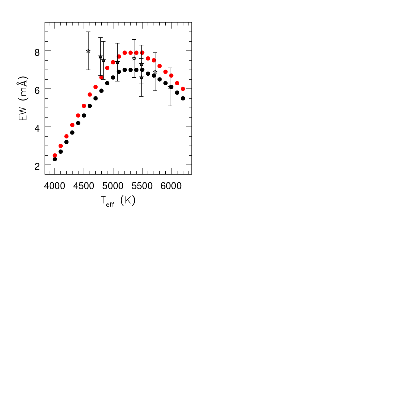
The individual dwarf O abundances, as well as those for the giants, are plotted with error bars in Figure 5. While the star-to-star dwarf abundances are in decent agreement within uncertainties, the plot reveals an apparent increase in O abundance with decreasing $T_{\rm eff}\;$for the three coolest dwarfs of the sample. Indeed, the trend is significant at the $\sim 99.5\%$ confidence level according to the linear correlation coefficient. Such a O abundance trend is not expected for open cluster stars, which are believed to be chemically homogeneous. In order to confirm the reality of the increasing O abundances with decreasing $T_{\rm eff}$, the expected line strengths of the $\lambda 6300$ feature, along with the observed EWs from Table 6, are plotted versus $T_{\rm eff}\;$in Figure 6. The expected line strengths have been determined by constructing synthetic spectra characterized by a single O abundance of $\log N(O)=8.83$ (the mean of the dwarfs with $T_{\mathrm{eff}}>5000\;\mathrm{K}$) and with Ni abundances of $\mathrm{[Ni/H]}=+0.13$ and $\mathrm{[Ni/H]}=+0.25$, the approximate Ni abundances of the six warmest and the three coolest stars, respectively (Table 5). Model atmospheres with $T_{\rm eff}\;$in the range $4000\leq T_{\mathrm{eff}}\leq 6200\;\mathrm{K}$, and with $\log g$ and $\xi$ calculated as described in Schuler et al. (2005), were interpolated from the OVER grids and used for the construction of the synthetic spectra. EWs of the synthesized $\lambda 6300$ features were measured using SPECTRE in the same manner as the observed lines. Excellent to good agreement exists between the observed and synthesized (with $\mathrm{[Ni/H]}=+0.13$) EWs for the six warmest stars of the sample. The observed EWs of the three coolest dwarfs start to deviate from the synthesized measurements, with the observed EW of the coolest Hyad, HIP 22654, $\sim 2.2\;\mathrm{m\AA}$ larger than expected (with $\mathrm{[Ni/H]}=+0.25$); this deviation for HIP 22654 is 2.2 times the adopted line strength uncertainty. These data support the notion that the O abundance increase among the cool dwarfs is statistically significant.

A growing body of evidence is emerging that suggests spectroscopic abundance analyses of cool ($T_{\mathrm{eff}}\lesssim 5500\;\mathrm{K}$) MS dwarfs making use of 1D, plane-parallel model atmospheres are unable to determine accurately the photospheric abundances of certain elements for these stars, with the abundance anomalies apparently increasing with decreasing $T_{\rm eff}$. Examples include the Fe II-Fe I abundance discrepancies in the Hyades (§3.3; Yong et al. 2004), M34 (Schuler et al., 2003), and UMa (King & Schuler, 2005); the high-excitation O I triplet-based O abundance trends in the Hyades (Schuler et al., 2005), the Pleiades and M34 (Schuler et al., 2004), UMa (King & Schuler, 2005), and chromospherically active stars (Morel & Micela, 2004); and excitation-related abundance differences between two K-dwarfs and the rest of the sample of nine M34 dwarfs (Schuler et al., 2003). The results of all of these studies point to the effects of overionization and excitation, possible phenomena in cool dwarfs that were first recognized by Feltzing & Gustafsson (1998). However, the [O I] $\lambda 6300$ feature results from a ground-state, magnetic dipole transition with a very weak electric quadrupole contribution, and its strength should be impervious to overionization/excitation effects. What, then, could be the cause of the apparent $T_{\rm eff}$-dependent increase in [O I]-based O abundances among the cool dwarfs of our sample?

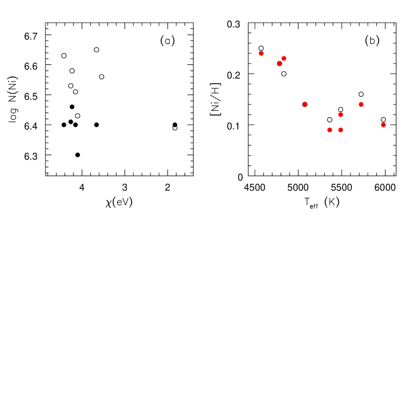
In an attempt to answer this question, attention is first turned to the blending Ni line(s) at 6300.34 Å, which results from a transition with a moderately-high, lower excitation potential of 4.27 eV and may be affected by the overexcitation effects discussed above. Care was taken to derive an accurate Ni abundance for each star, so that the contribution of the Ni blend to the measured EW of the $\lambda 6300$ line could be determined. The Ni lines chosen for measurement have lower excitation potentials in the range $1.83\leq\chi\leq 4.42\;\mathrm{eV}$, with all but one line having $\chi\geq 3.54\;\mathrm{eV}$. The absolute Ni abundances of the warmest star in the sample (HIP 19148; 5978 K) and of the coolest star in the sample (HIP 22654; 4573 K) are plotted as a function of $\chi$ in Figure 7a. The Ni abundances of HIP 19148 are independent of $\chi$, while those for HIP 22654 derived from high-excitation lines are $\sim 0.15\;\mathrm{dex}$ higher than that derived from the low-excitation line, evincing clearly $\chi$-dependent abundances in at least the coolest star. In response, the relative Ni abundance of each star has been re-derived from a set of 3-5 Ni lines with $\chi$ ranging from 4.23-4.26 eV (Table 8); the Ni abundance from these lines will presumably provide a better indication of the line strength of the 4.27 eV Ni line blend and thus of its contribution to the $\lambda 6300$ EW. The resulting mean abundances, along with the originally accepted [Ni/H] abundances, are plotted for each star versus $T_{\rm eff}\;$in Figure 7b. Although an unequivocal $T_{\rm eff}$-dependent increase in Ni abundances with decreasing $T_{\rm eff}\;$is apparent, no appreciable difference between the two abundance measures is seen. Thus, the [O I] abundance trend does not appear to be the result of the Ni blend and overexcitation effects.

Another possible cause of the increase in [O I] abundances in the cool dwarfs could be related to overionization/excitation effects, namely an actual increase in the number of O atoms in the photospheres of the cool dwarfs due to greater than predicted dissociation of O-containing molecules, especially CO, the most prominent O-containing molecule in the photospheres of our program stars. The larger than predicted EWs of the $\lambda 6300$ [O I] line measured in the spectra of the cool dwarfs would be a natural consequence of an increased number of O atoms that would result from the dissociation of molecules, and not accounting for this in the abundance derivations would lead to larger than expected abundances. The plausibility of this scenario has been investigated by rederiving the O abundances of each dwarf and excluding CO from the molecular equilibrium calculations performed by MOOG, effectively simulating the complete dissociation of CO in the stellar photospheres. Astonishingly, the resulting O abundances of the cool stars are brought into excellent agreement with those of the warm stars, as can be seen in Figure 8. The mean of these newly derived abundances is $\mathrm{[O/H]}=0.12$ with a standard deviation of only 0.03 dex. The results of this exercise in themselves are of little scientific value; however, they do provide significant motivation to investigate O abundances derived from molecular spectral lines: if $T_{\rm eff}$-dependent overdissociation of O-containing molecules is occurring in the photospheres of cool dwarfs, one would expect to see O abundances derived from molecular lines exhibit a trend of decreasing abundances with decreasing $T_{\rm eff}$, in contrast to the increasing abundances with decreasing $T_{\rm eff}\;$observed in the O abundances derived from atomic lines.

Accordingly, O abundances of four Hyades dwarfs (HIP 19148, HIP 19793, HIP 21099, and HD 29159) have been derived via spectral synthesis of the near-UV, $\lambda 3167$ OH line ($\chi=1.11\;\mathrm{eV}$) in high-quality ($\mathrm{S/N}\approx 100$, $R\approx 45,000$) spectra obtained with the Keck I telescope and HIRES spectrograph. Abundances derived from molecular species are highly temperature sensitive, and molecular lines in the UV may be affected by NLTE effects (Hinkle & Lambert, 1975) and contributions of metals to the continuous opacity (Allende Prieto et al., 2003). Nonetheless, LTE analyses of near-UV OH lines have been shown to produce reliable results (Israelian et al., 1998). For the present study, using OH ought to be a good choice to test for the effects of overdissociation because (1) it has a lower dissociation energy ($D_{0}=4.39\;\mathrm{eV}$) compared to that of the more multitudinous CO ($D_{0}=11.09\;\mathrm{eV}$); and (2) even a small amount of overdissociation will affect significantly the observed line strengths due to the relatively lower number abundance of OH molecules in the atmospheres of late-G and early-K dwarfs. The near-UV spectra of HIP 19148, HIP 19793, and HIP 21099 are those from the study of Boesgaard & King (2002), and the data are fully described therein. The near-UV spectrum of HD 29159 was obtained on 2004 Dec 15 with Keck I and HIRES, using the “b” configuration; a resolution of $R\approx 45,000$ and a $\mathrm{S/N}\approx 80$ at 3167 Å were achieved. The observations made use of the new three-chip ($2048\times 4096$ each) CCD mosaic. Identifying clean spectral lines in the near-UV is difficult due to the considerable number of identified and unidentified blends. The selection of OH lines compiled by the related studies of Israelian et al. (1998) and Israelian et al. (2001) was used as a starting point for identifying acceptable lines in our spectra, and the $\lambda=3167.169\;\mathrm{\AA}$ line was found to be the most promising candidate. While this line is surely contaminated by blends, OH is the dominant contributor, and the feature should provide a good indication of relative abundance differences, if present. It should be stressed that we are not attempting to determine accurate O abundances from the analysis of the OH feature; rather, the goal is to determine if relative, star-to-star abundance differences are observed. The spectral synthesis was carried out with MOOG and an initial line list compiled from the VALD database. Final $gf$-values for the OH and surrounding lines were determined by fitting the region for the Sun using the Kurucz solar atlas flux spectrum (Kurucz et al., 1984) and adopting an input O abundance of $\log N(O)=8.69$, the solar abundance derived from the $\lambda 6300$ [O I] line in our high-quality McDonald 2.7-m spectrum of the daytime sky. The Kurucz solar spectrum was smoothed by convolving it with a Gaussian profile with a FWHM of 0.052 Å (García López, Rebolo, & Pérez de Taoro, 1995).

Synthetic fits to the observed spectra of the four Hyads are quite satisfactory and are presented in Figure 9. The synthetic spectra have been smoothed using Gaussians with FWHM values determined via a cross-correlation analysis using the fxcor utility within IRAF. Numerous synthetic spectra of the 3167 Å region for a fiducial Hyades dwarf having $T_{\rm eff}=5500\;{\rm K}$ and ${\rm[Fe/H]}=+0.13$, each broadened with a Gaussian of differing FWHM, were cross-correlated with the observed Kurucz solar spectrum as a template. The resulting cross-correlation function (CCF) widths were then plotted versus the input FWHM smoothing values of the synthetic Hyades spectrum, and a fourth order polynomial was fit to this relation. Our observed Keck/HIRES Hyades spectra were then cross-correlated with the Kurucz solar spectrum, the CCF width measured, and the appropriate FWHM determined from our synthetic relation. In Figure 9, the final absolute O abundance that resulted in the best fit for each star is included, as well as syntheses for $\log N(O)=8.46$ and $\log N(O)=9.36$. Close inspection reveals a gradual migration of the observed OH line from near the synthesis characterized by the low O abundance ($\log N(O)=8.46$) in Figure 9a (HIP 19148, the warmest star) toward the synthesis characterized by the high O abundance ($\log N(O)=9.36$) in Figure 9d (HD 29159, the coolest star), suggesting an increase in the O abundance with decreasing $T_{\rm eff}$. This behavior is confirmed in Figure 10, where the OH-derived O abundances are plotted versus $T_{\rm eff}$, and is contrary to the expected result if overdissociation of O-containing molecules is occurring. This leads to the conclusion that the increasing [O I] abundances among the cool dwarfs is not the result of overdissociation of O-containing molecules, although additional OH data for Hyades dwarfs cooler than $\sim 5000\;\mathrm{K}$ are desirable for greater confirmation or alternatively, to determine if the abundances continue to increase at lower $T_{\rm eff}$.

The nature of the observed increase in O abundances as derived from the $\lambda 6300$ [O I] feature remains uncertain. Further study of this phenomenon will benefit greatly from additional data for dwarfs with $T_{\rm eff}\;$as cool as 4200 K, where the expected EWs of the [O I] feature for Hyades metallicity stars are $>3\;\mathrm{m\AA}$ (Figure 4) and should be measurable in high-quality spectra. Consequently, if the EWs are indeed enhanced in the spectra of dwarfs cooler than those study here, then future analyses could be extended to even cooler $T_{\rm eff}$. Regardless, a caveat must be extended: current abundance derivations for cool dwarfs, irrespective of the lower excitation potential of the spectral lines being employed, should be received with caution. Hyades dwarf O abundances as derived from the $\lambda 6300$ [O I], near-IR $\lambda 7774$ triplet, and the $\lambda 3167$ OH line are provided in Figure 10. The [O I] and OH-based dwarf abundances of the warmest stars agree nicely. The triplet-based dwarf O abundances of the warm stars are offset by $\sim 0.10$ dex (Figure 5), similar to the $\sim 0.10$ dex difference in the Fe II-Fe I abundances in the warmest stars (Figure 3). The reason for the offsets is not clear but might be related to NLTE effects or undetermined internal or systematic errors (Schuler et al., 2005). Below about 5000 K, the [O I] and triplet abundance trends clearly diverge, but both show signs of increasing with decreasing $T_{\rm eff}$. Previous, as well as the current, studies have reported abundance trends among cool cluster dwarfs that present a coherent picture of overionization/excitation related effects (Figure 3, Figure 7, Schuler et al. 2005, Yong et al. 2004, etc.), and Schuler et al. (2005) have demonstrated the plausibility that the effects might be the result of temperature inhomogeneities due to the presence of photospheric spots, faculae, and/or plages. The [O I]-derived abundance trend presented here does not fit into this scenario, and if confirmed, additional mechanisms to explain the behavior will be required.

Conversely, the O abundances of the six warm dwarfs ($5075\leq T_{\mathrm{eff}}\leq 5978$) in our sample are in excellent agreement and do not engender incertitude in their accuracy. Using the abundances of these six warm dwarfs, excluding those of the three coolest due to their uncertainty, an O abundance of $[\mathrm{O/H}]=+0.14\;\pm 0.02$ (uncertainty in the mean) is found for the Hyades cluster. This abundance agrees near-perfectly with that found by KH96, $[\mathrm{O/H}]=+0.15\;\pm 0.01$; although the agreement is difficult to explain. HIP 20082 ($T_{\mathrm{eff}}=4784$), the one star in common to KH96 and the present study, is not included in the cluster mean here. An absolute abundance of $\log N(O)=9.09$ for HIP 20082 was derived by KH96, whereas we find $\log N(O)=8.96$; however, the absolute solar abundances of the two studies differ by 0.24 dex, resulting in a study-to-study difference of 0.11 dex in the relative O abundances for HIP 20082. This difference can be attributed to the combined effects of small differences in stellar parameters, EWs, and sensitivities to changes in the $\log gf$-values of the [O I] and Ni lines. Thus, it seems the analysis of each study has conspired to provide the same cluster abundance despite the difference in the relative abundances for the one star in common.

4.2 O in Hyades Giants

The O abundances derived for the Hyades giants are in good star-to-star agreement (Table 6) and have a mean value of $\mathrm{[O/H]}=+0.08\;\pm 0.02$ (uncertainty in the mean). This is 0.16 dex higher than the mean giant abundance obtained by KH96; the difference can be attributed to the complex interplay of the discordance in adopted solar abundances, the updated atomic parameters for the [O I] and Ni blend lines, and small disagreements in EWs. The differences between our measured EWs and those used by KH96, which are means of the values of Lambert & Ries (1981), Kjaergaard et al. (1982), and Gratton (1985), average about 2.9 mÅ and are within the combined uncertainties.

Oxygen abundances derived from the near-IR, high-excitation $\lambda 7774$ O I triplet for both unevolved and evolved stars alike are known to be influenced by NLTE effects (e.g., King & Boesgaard 1995; Cavallo, Pilachowski, & Rebolo 1997). Nevertheless, deriving O abundances from these lines can be informative. EWs of the triplet as measured in the high-quality McDonald 2.7-m spectra of the three Hyades giants are given in Table 9. Contrary to expectations, the EW of the central line of the triplet ($\lambda=7774.16\;\mathrm{\AA}$) is larger than the blue line ($\lambda=7771.95\;\mathrm{\AA}$), suggesting the presence of a blend that is otherwise negligible for dwarfs. No asymmetry of the central line is seen in the McDonald spectra (Figure 11), but a blending feature might be present, possibly a Fe I line at 7774.00 Å (Takeda et al., 1998). LTE abundances (Table 9) were derived utilizing the same model atmospheres as for the [O I] analysis; atomic parameters for the triplet are those used by Schuler et al. (2005). Excluding the central line from further analysis, the giant LTE mean O abundances derived from the remaining two lines of the triplet are approximately 0.28 dex higher than those derived from the [O I] line, qualitatively in-line with NLTE calculations. NLTE corrections to the LTE abundances have been estimated using the results of Takeda (2003) who performed extensive NLTE calculations for a large collection of model atmosphere parameters for late-F through early-K stars. The NLTE corrections are available for only discrete steps in $T_{\rm eff}$, $\log g$, and $\xi$, and thus a mean of the corrections from two separate grid steps has been taken here. The corrections for the Hyades giants have been determined using the values for the parameter sets of $T_{\mathrm{eff}}=5000\;\mathrm{K}$, $\log g=2.00$, $\xi=1.00\;\mathrm{km}\;\mathrm{s}^{-1}$ and $T_{\mathrm{eff}}=5000\;\mathrm{K}$, $\log g=3.00$, $\xi=1.00\;\mathrm{km}\;\mathrm{s}^{-1}$. The resulting NLTE abundances are included in Table 9, and both LTE and NLTE abundances are plotted in Figure 10. We calculate a mean NLTE abundance, excluding the abundance derived from the central line, for the giants of $\mathrm{[O/H]}=0.17\;\pm 0.02$ (uncertainty in the mean). This result is in satisfactory accordance with the [O I] giant abundances and adds muster to the super-solar O abundances found here.

4.3 Is There a Hyades Giant-Dwarf O Abundance Discrepancy?

With mean O abundances for both the dwarfs and giants comfortably in hand, we can now proceed to address the question of the so-called Hyades giant-dwarf oxygen discrepancy initially reported by KH96. KH96 derived relative abundances of 0.15 and -0.08 dex for the dwarfs and giants, respectively, resulting in a 0.23 dex O abundance difference. Our analysis does not confirm this large abundance discordance; the mean O abundances derived for the dwarfs and giants are 0.14 and 0.08 dex, reducing the difference to only 0.06 dex. Furthermore, the abundances of the warm dwarfs ($T_{\mathrm{eff}}>5000\;\mathrm{K}$) and of the giants are in good star-to-star agreement (Figure 5), and the samples are statistically indistinguishable. We note that the low O abundance ($\mathrm{[O/H]}=-0.08\pm 0.01$) derived for the giants by KH96 is in near-perfect agreement with the value ($\mathrm{[O/H]}=-0.06\pm 0.15$) obtained by García López et al. (1993) via an NLTE analysis of the triplet in the spectra of 25 Hyades F dwarfs. While these results present a resolution to the giant-dwarf O discrepancy as well, they suggest a lower cluster O abundance than found here and by others (King 1993; Schuler et al. 2005; Boesgaard 2005). Given our consistently super-solar O abundances derived from the various features considered, we believe our values to be more accurate.

The agreement between the dwarf and giant O abundances corroborates the conclusion reached from our evolutionary model of a 2.5 $M_{\sun}$ star described in §1.1, i.e., the Hyades giants have not mixed O-depleted material into their atmospheres, a possible cause of the giant-dwarf O abundance discrepancy suggested by KH96. Instead, the culprit seems to have been systematic errors related primarily to the treatment of the Ni blend of the $\lambda 6300$ feature, as described in Sections 3.4.1, 4.1, and 4.2. This reanalysis of the giant-dwarf oxygen discrepancy seemingly demonstrates that even careful relative abundance studies can lead to erroneous results.

5 SUMMARY

We have analyzed the $\lambda 6300$ [O I] spectral feature in high-quality spectra obtained with the VLT Kueyen (UT2) telescope at the European Southern Observatory, Paranal and the Harlan J. Smith and Otto Struve telescopes at The McDonald Observatory in order to revisit the Hyades Giant-Dwarf Oxygen Discrepancy initially reported by King & Hiltgen (1996). Abundances of Fe, Ni, and O have been derived for nine Hyades dwarfs and three Hyades giants using two sets of model atmosphere grids based on the Kurucz ATLAS9 code. All results are found to be independent of model atmosphere, as previously demonstrated for MS dwarfs (Schuler et al., 2004) but shown for the first time for red giant stars here. Dwarf Fe abundances derived from singly ionized lines are generally found to be greater than those derived from neutral lines, with the discrepancy increasing with decreasing $T_{\rm eff}$; this result confirms the original espial by Yong et al. (2004). No such discordance is observed for the giants, for which ionization balance is achieved within uncertainties. Mean Fe abundances from Fe I lines alone are 0.08 and 0.16 for the dwarfs and giants, respectively. Both of these values are in good agreement with previous determinations for the Hyades.

Our O abundance analysis has improved on that of King & Hiltgen most significantly in the treatment of the Ni I line that is blended with the [O I] feature. Johansson et al. (2003) has shown experimentally that the Ni blend is actually due to two isotopic components, and the weighted $gf$-value for each component has been subsequently calculated by Bensby et al. (2004). The weighted isotopic values have been used here. Our resulting solar abundance, based on an equivalent width of the [O I] line measured in a high-quality spectrum of the day-time sky at The McDonald Observatory, is $\log N(O)=8.69$, in excellent agreement with the results of Allende Prieto et al. (2001) and of Asplund et al. (2004), both of which make use of a three-dimensional, time-dependent hydrodynamical model of the solar atmosphere. The solar abundance of King & Hiltgen is 0.24 dex greater than that found here; it is shown that this large difference can be almost entirely attributed to the updated $gf$-value of the Ni blend.

The dwarf O abundances based on the [O I] feature are in agreement within uncertainties, but an apparent trend of increasing abundances with decreasing $T_{\rm eff}\;$is observed among the three coolest dwarfs of the sample. Possible explanations for the anomalous abundances include a greater than expected contribution to the EW of the $\lambda 6300$ feature from the Ni blend ($\chi=4.27\;\mathrm{eV}$) due to overexcitation-related effects and/or an increase in the amount of atomic O due to overdissociation of O-containing molecules. Both of these possibilities are investigated, but neither are found to be viable. Analysis of the [O I] line in the spectra of additional cool open cluster dwarfs is recommended to confirm the abundance trend found here. Using the abundances of the six warmest dwarfs in the sample, we find a mean value of $\mathrm{[O/H]}=+0.14\;\pm 0.02$. Our dwarf O abundance is in excellent agreement with that of King & Hiltgen, despite considerable differences in the analyses.

Analysis of the [O I] feature in spectra of the Hyades giants results in a mean abundance of $\mathrm{[O/H]}=+0.08\;\pm 0.02$. This is 0.16 dex higher than the value obtained by King & Hiltgen; the difference is again mainly due to the updated $gf$-value of the Ni blend. We also derive O abundances for the giants from the near-IR, high-excitation triplet. The NLTE corrections of Takeda (2003) have been adopted, and the resulting mean NLTE abundance is $\mathrm{[O/H]}=+0.17$ and is in satisfactory accordance with the giant and dwarf [O I]-based measurements. Comparing the dwarf and giant mean O abundances, we do not confirm the Giant-Dwarf Oxygen Discrepancy initially reported by King & Hiltgen. The abundance difference found by King & Hiltgen seems to have resulted primarily from systematic errors related to the $gf$-value of the Ni blend, which was poorly constrained at that time.

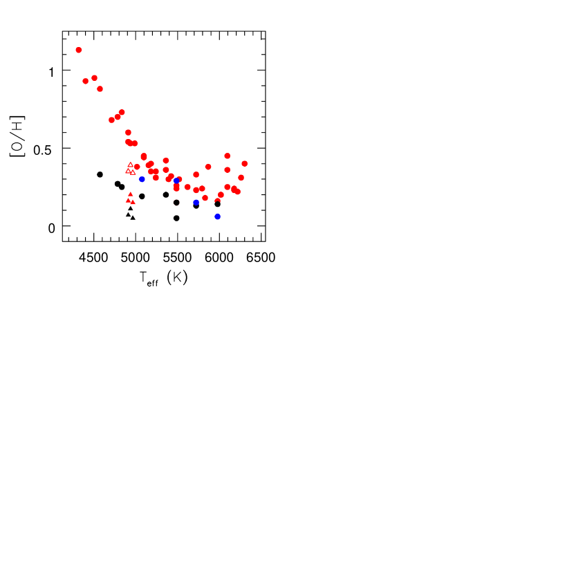
In closing, a summation of the Hyades cluster O abundance derived from the myriad indicators is in order. The totality of our results are given in Figure 10, where the dwarf LTE O abundances as derived from the high-excitation O I triplet from Schuler et al. (2005) are also plotted. The figure presents a convoluted and possibly discouraging picture with regards to O abundance derivations, but all hope is not lost. The $\lambda 6300$ [O I] line appears to remain the best indicator of O abundances in the atmospheres of both dwarfs (black circles) and giants (black triangles), although some monition is required for dwarfs with $T_{\mathrm{eff}}\lesssim 5000\;\mathrm{K}$. Abundances derived from the high-excitation triplet exhibit rich behavior in both dwarfs (red circles) and giants (red triangles). For the dwarfs with $T_{\mathrm{eff}}\gtrsim 6100\;\mathrm{K}$ and the giants, the LTE abundances are in accord with current NLTE expectations (Takeda, 2003). Indeed, applying the NLTE corrections appropriate for the Hyades giants from the extensive collection of Takeda (2003) brings their triplet abundances into close agreement with their [O I] abundances. The behavior of the LTE triplet abundances of the cool dwarfs ($T_{\mathrm{eff}}\lesssim 5450\;\mathrm{K}$), on the other hand, are not predicted by current NLTE calculations; Schuler et al. (2005) showed that temperature inhomogeneities due to spots, faculae, and/or plages might be a plausible explanation for the cool dwarf O abundance anomalies. At intermediate $T_{\rm eff}\;$($5450\lesssim T_{\mathrm{eff}}\lesssim 6100\;\mathrm{K}$), no discordance between triplet and [O I] abundances is expected, especially if the abundances are given relative to solar. As discussed in §4.1, the significance of the $\sim 0.10$ dex offset between the abundances from these two indicators is not clear, but may be related to NLTE effects or systematic errors. Relatedly, Boesgaard (2005) recently derived O abundances using an LTE analysis of the triplet for 18 Hyades dwarfs in the intermediate $T_{\rm eff}\;$range given above and found a mean abundance of $\mathrm{[O/H]}=+0.17\pm 0.01$, a value intermediate to the triplet abundance of (Schuler et al., 2005) and the [O I] abundance found here. Deriving abundances from a single near-UV OH line (blue circles) can be precarious given uncertainties associated with ill-constrained atomic parameters, high sensitivities to stellar parameters, and continuum placement; nevertheless, the trend of increasing OH-based abundances with decreasing $T_{\rm eff}\;$we find is reminiscent of those based on the triplet and [O I] line. Finally, combining the [O I] results for both the warm dwarfs ($T_{\mathrm{eff}}\gtrsim 5000\;\mathrm{K}$) and the giants, a cluster abundance of $\mathrm{[O/H]}=+0.12\;\pm 0.02$ is achieved, giving the best indication of the Hyades O abundance.

Figure 1: Stellar structure as a function of time from the 2.5 $M_{\sun}$ model with an initial Hyades-like composition. Time measured as the difference between total elapsed time of the model ($\mathrm{t}_{\mathrm{f}}\approx 7.9\times 10^{8}\;\mathrm{yr}$) and time (t) from $\mathrm{t}=0$ is plotted on a logarithmic scale along the abscissa. Convective regions are given in gray, and radiative regions are white.

Figure 2: Isotopic abundances of the surface of the 2.5 $M_{\sun}$ model with an initial Hyades-like composition as a function of time. The top panel shows the evolution of the ${}^{12}\mathrm{C}$/${}^{13}\mathrm{C}\;$ratio, while the bottom panel displays the evolution of the ${}^{16}\mathrm{O}\;$(solid line) and ${}^{12}\mathrm{C}\;$abundances (dashed line).

Figure 3: Difference in Fe abundances derived from Fe II and Fe I lines plotted against $T_{\rm eff}$. The abundance differences for the dwarfs are given as circles and those for the giants as stars.

Figure 4: VLT/UVES and McDonald 2.7-m/2dcoudé spectra of the $\lambda 6300$ [O I] region for the Hyades dwarf sample. The [O I] line is marked by the arrow.

Figure 5: Relative LTE O abundances of Hyades dwarfs (circles) and giants (stars) versus $T_{\rm eff}$. The error bars represent the total internal uncertainties as described in the text.

Figure 6: Equivalent widths of the $\lambda 6300$ [O I] feature for the Hyades dwarf sample versus $T_{\rm eff}$. Open stars with error bars are the observed EWs. Closed circles are EWs measured from synthetic spectra with input Ni abundances of $\mathrm{[Ni/H]}=+0.13$ (black) and $\mathrm{[Ni/H]}=+0.25$ (red).

Figure 7: (a) Line-by-line absolute Ni abundances plotted against $T_{\rm eff}$. Filled circles are the abundances for HIP 19148, the warmest dwarf in the sample ($T_{\mathrm{eff}}=5978\;\mathrm{K}$); open circles are the abundances of HIP 22654, the coolest dwarf in the sample ($T_{\mathrm{eff}}=4573\;\mathrm{K}$). (b) Relative Ni abundances of the Hyades dwarf sample versus $T_{\rm eff}$. Ni abundances derived with the original set of lines (Table 2) are given as open circles; red circles are the abundances derived with a set of Ni lines with $4.23\leq\chi\leq 4.26\;\mathrm{eV}$, values that are approximately equal to that ($\chi=4.27\;\mathrm{eV}$) of the Ni I line blended with the $\lambda 6300$ [O I] feature.

Figure 8: Relative LTE O abundances as a function of $T_{\rm eff}$. Closed circles are the original abundances, as shown in Figure 5. Oxygen abundances derived without including CO in molecular equilibrium calculations- effectively simulating the complete dissociation of the CO molecule- are given as open circles.

Figure 9: Keck/HIRES spectra (closed circles) and synthetic fits (solid lines) of the near-UV, $\lambda 3167$ OH line for four Hyades dwarfs. The abundance of the best fit is given in each panel. The low and high abundance syntheses are the same for each panel and are characterized by $\log N(O)=8.46$ and $\log N(O)=9.36$. A solar O abundance of $\log N(O)=8.69$- the abundance derived from the $\lambda 6300$ [O I] line in our high-quality McDonald 2.7-m spectrum of the daytime sky- has been adopted for this analysis.

Figure 10: Compilation of Hyades O abundances versus $T_{\rm eff}$. LTE Dwarf abundances are given as circles and are derived from the $\lambda 3167$ OH feature (blue), the $\lambda 6300$ [O I] line (black), and the high-excitation triplet (red; data taken from Schuler et al. 2005). Giant abundances are shown as triangles; the abundances are derived assuming LTE from the $\lambda 6300$ [O I] line (closed black) and the high-excitation triplet (open red). Giant triplet abundances subjected to the NLTE corrections of Takeda (2003) are also given (closed red).

Figure 11: McDonald 2.7-m/2dcoudé spectra of the high-excitation triplet region for the Hyades giants $\gamma\;\mathrm{Tau}$, $\delta\;\mathrm{Tau}$, and $\epsilon\;\mathrm{Tau}$. The triplet is marked by the arrows.

Table 1: Cross-Identifications & Observing Log

								Date	Exp	Int. Time
HIP		HD		Other		Telescope		UT	#	(s)	S/N
$14976\dotfill$		19902		$\cdots$		McD		12 Oct 2004	1	1800	225
$19148\dotfill$		25825		$\mathrm{vB}\;10$		VLT		18 Jan 2003	3	120	350
$19793\dotfill$		26736		$\mathrm{vB}\;15$		McD		12 Oct 2004	1	840	175
$20082\dotfill$		285690		$\mathrm{vB}\;25$		VLT		18 Jan 2003	3	300	255
$20949\dotfill$		283704		$\mathrm{vB}\;76$		VLT		18 Jan 2003	2	285	240
$21099\dotfill$		28593		$\mathrm{vB}\;87$		VLT		18 Jan 2003	3	220	330
$22654\dotfill$		284930		$\cdots$		VLT		18 Jan 2003	2	600	235
$23312\dotfill$		$\cdots$		$\mathrm{BD}+04\;810$		VLT		14 Oct 2002	2	340	240
$\cdots$		29159		$\mathrm{vB}\;99$		VLT		18 Jan 2003	3	400	340
$20205\dotfill$		27371		$\gamma\;\mathrm{Tau}$		McD		Multiple	$\cdots$	$\cdots$	$\cdots$
$20455\dotfill$		27697		$\delta\;\mathrm{Tau}$		McD		Multiple	$\cdots$	$\cdots$	$\cdots$
$20889\dotfill$		28305		$\epsilon\;\mathrm{Tau}$		McD		Multiple	$\cdots$	$\cdots$	$\cdots$
$\mathrm{Sun}\dotfill$		$\cdots$		$\cdots$		McD		10 Oct 2004	1	30	950

Table 2: Stellar Parameters

		$B-V$		$T_{\mathrm{eff}}$		$\log g$		$\xi$
Star		Mag.		(K)		(cgs)		(km $\mathrm{s}^{-1}$)
$\mathrm{HIP}\;14976$		0.73		5487		4.54		1.24
$\mathrm{HIP}\;19148$		0.59		5978		4.44		1.45
$\mathrm{HIP}\;19793$		0.66		5722		4.49		1.34
$\mathrm{HIP}\;20082$		0.98		4784		4.65		1.00
$\mathrm{HIP}\;20949$		0.77		5361		4.56		1.20
$\mathrm{HIP}\;21099$		0.73		5487		4.54		1.24
$\mathrm{HIP}\;22654$		1.07		4573		4.68		1.00
$\mathrm{HIP}\;23312$		0.96		4834		4.64		1.02
$\mathrm{HD}\;29159\dotfill$		0.87		5075		4.61		1.09
$\gamma\;\mathrm{Tau}\dotfill$		0.99		4965		2.63		1.32
$\delta\;\mathrm{Tau}\dotfill$		0.98		4938		2.69		1.40
$\epsilon\;\mathrm{Tau}\dotfill$		1.01		4911		2.57		1.47
$\mathrm{Sun}\dotfill$				5777		4.44		1.38

Table 3: Fe & Ni Equivalent Widths- Dwarfs

							Equivalent Widths ($\mathrm{m\AA}$)
	$\lambda_{\mathrm{rest}}$		$\chi$						HIP									HD
Ion	(Å)		(eV)		$\log gf$		$\mathrm{EW}_{\sun}$		14976	19148	19793	20082	20949	21099	22654	23312		29159
Fe I…	5807.79		3.29		-3.41		9.9		15.7	$\cdots$	14.8	23.3	17.5	15.6	23.7	22.1		20.0
	5853.16		1.49		-5.28		8.9		15.4	7.33	10.7	29.5	18.2	17.0	36.1	28.4		24.5
	6054.08		4.37		-2.31		10.9		16.4	10.4	18.5	19.4	16.5	16.8	18.0	19.3		18.4
	6120.25		0.91		-5.95		6.53		12.3	$\cdots$	9.7	25.5	13.0	11.7	34.7	24.6		19.7
	6159.38		4.61		-1.97		14.2		21.7	15.4	17.7	26.0	21.6	21.8	27.6	25.1		25.2
	6290.53		2.59		-4.33		6.26		15.2	$\cdots$	8.3	17.2	10.6	10.4	17.4	16.5		14.5
	6385.73		4.73		-1.91		12.5		16.9	$\cdots$	16.6	22.9	20.0	17.9	24.7	22.3		20.0
	6591.33		4.59		-2.07		11.4		17.4	10.9	13.7	19.5	17.3	18.4	18.1	21.2		20.0
	6608.04		2.28		-4.03		19.4		28.5	17.2	25.1	44.4	33.3	31.6	44.8	43.6		39.6
	6646.97		2.61		-3.99		10.6		18.3	$\cdots$	16.9	29.1	19.7	20.3	30.1	30.4		26.0
	6739.52		1.56		-4.95		12.9		21.2	$\cdots$	15.8	38.9	$\cdots$	22.9	42.1	34.6		31.1
	6746.98		2.61		-4.35		5.37		9.4	$\cdots$	7.7	16.7	10.3	$\cdots$	17.2	13.6		12.3
	6837.01		4.59		-1.81		19.2		26.6	18.7	25.2	29.0	25.6	26.7	26.4	28.2		27.7
Fe II…	5425.25		3.20		-3.21		41.6		44.3	52.4	51.4	$\cdots$	40.6	42.1	31.9	$\cdots$		33.6
	6084.10		3.20		-3.80		21.5		22.9	29.4	28.7	12.2	22.8	21.6	8.4	$\cdots$		15.0
	6149.25		3.89		-2.72		40.1		35.9	50.1	46.2	20.1	36.0	37.2	18.8	22.0		26.4
	6247.56		3.89		-2.31		59.2		56.1	69.7	67.4	27.4	55.1	53.5	21.0	33.0		38.9
	6432.68		2.89		-3.58		43.0		$\cdots$	54.6	$\cdots$	25.7	39.0	41.2	22.3	25.8		31.7
	6456.39		3.90		-2.08		66.1		68.5	82.3	81.4	36.0	61.4	65.1	26.2	41.1		48.1
Ni I…	6130.14		4.26		-0.96		22.0		31.6	25.0	28.6	29.0	30.7	30.2	28.1	34.3		31.6
	6133.98		4.09		-1.83		7.21		9.5	$\cdots$	$\cdots$	11.5	$\cdots$	$\cdots$	$\cdots$	10.4		8.8
	6177.25		1.83		-3.50		17.7		24.5	15.6	22.3	35.1	25.6	25.5	34.4	33.3		31.0
	6223.99		4.10		-0.91		28.4		39.4	29.2	38.7	36.7	37.0	37.6	34.0	36.8		38.4
	6370.36		3.54		-1.94		15.4		22.8	$\cdots$	20.5	$\cdots$	23.2	24.1	22.2	24.2		24.5
	6414.59		4.15		-1.18		19.3		26.3	20.4	$\cdots$	25.2	27.2	25.5	22.9	28.1		26.7
	6598.61		4.23		-0.98		26.9		35.3	28.5	34.3	35.4	34.3	36.2	30.7	34.8		34.4
	6635.14		4.42		-0.82		25.9		37.5	25.3	34.1	33.8	36.1	37.0	30.7	34.3		34.9
	6842.04		3.66		-1.48		28.3		39.3	27.6	37.4	42.4	38.1	37.9	41.3	39.9		41.8

Table 4: Fe & Ni Equivalent Widths- Giants

	$\lambda_{\mathrm{rest}}$		$\xi$						Equivalent Widths ($\mathrm{m\AA}$)
Ion	$\mathrm{\AA}$		(eV)		$\log gf$		$\mathrm{EW}_{\sun}$		$\gamma\;\mathrm{Tau}$		$\delta\;\mathrm{Tau}$		$\epsilon\;\mathrm{Tau}$
Fe I…	5853.16		1.49		-5.28		8.9		47.9		51.4		55.9
	6054.08		4.37		-2.31		10.9		32.7		36.1		37.2
	6120.25		0.91		-5.95		6.53		44.8		44.8		54.7
	6159.38		4.61		-1.97		14.2		40.0		37.7		$\cdots$
	6290.53		2.59		-4.33		6.26		35.8		37.1		39.1
	6385.73		4.73		-1.91		12.5		33.1		35.8		40.8
	6591.33		4.59		-2.07		11.4		30.7		35.5		42.3
	6608.04		2.28		-4.03		19.4		66.7		72.4		76.3
	6646.97		2.61		-3.99		10.6		59.0		59.4		68.5
	6739.52		1.56		-4.95		12.9		64.1		62.9		72.4
	6746.98		2.61		-4.35		5.37		32.5		31.4		38.8
	6837.01		4.59		-1.81		19.2		49.5		50.2		55.4
Fe II…	5425.25		3.20		-3.21		41.6		67.4		67.0		69.8
	6084.10		3.20		-3.80		21.5		47.6		48.0		48.9
	6149.25		3.89		-2.72		40.1		55.3		54.9		58.5
	6247.56		3.89		-2.31		59.2		77.3		76.6		79.7
	6456.39		3.90		-2.08		66.1		89.2		90.3		91.1
Ni I…	6130.14		4.26		-0.96		22.0		49.8		52.6		58.8
	6133.98		4.09		-1.83		7.21		26.2		23.1		23.5
	6223.99		4.10		-0.91		28.4		66.3		61.3		$\cdots$
	6598.61		4.23		-0.98		26.9		55.6		56.2		64.1
	6635.14		4.42		-0.82		25.9		63.9		60.2		66.9
	6842.04		3.66		-1.48		28.3		68.4		70.5		71.3

Table 5: Final Fe and Ni Abundances

		[Fe I/H]						[Fe II/H]						[Ni I/H]
Star		OVER	$\sigma$		MLT5	$\sigma$		OVER	$\sigma$		MLT5	$\sigma$		OVER	$\sigma$		MLT5	$\sigma$
$\mathrm{HIP}\;14976$		0.07	0.03		0.08	0.03		0.26	0.05		0.27	0.05		0.13	0.03		0.13	0.03
$\mathrm{HIP}\;19148$		0.10	0.04		0.09	0.03		0.18	0.07		0.18	0.07		0.11	0.03		0.10	0.03
$\mathrm{HIP}\;19793$		0.13	0.03		0.13	0.03		0.29	0.05		0.30	0.05		0.16	0.03		0.16	0.03
$\mathrm{HIP}\;20082$		0.09	0.03		0.10	0.03		0.52	0.11		0.49	0.12		0.22	0.04		0.22	0.04
$\mathrm{HIP}\;20949$		0.04	0.03		0.05	0.03		0.32	0.07		0.32	0.09		0.11	0.04		0.12	0.04
$\mathrm{HIP}\;21099$		0.08	0.04		0.09	0.04		0.22	0.08		0.23	0.07		0.13	0.04		0.14	0.04
$\mathrm{HIP}\;22654$		0.14	0.04		0.15	0.04		0.74	0.14		0.69	0.13		0.25	0.05		0.24	0.04
$\mathrm{HIP}\;23312$		0.07	0.03		0.08	0.03		0.53	0.09		0.51	0.10		0.20	0.03		0.21	0.04
$\mathrm{HD}\;29159\dotfill$		0.04	0.03		0.05	0.03		0.37	0.09		0.35	0.09		0.14	0.04		0.14	0.04
$\gamma\;\mathrm{Tau}\dotfill$		0.14	0.08		0.15	0.08		0.22	0.16		0.23	0.15		0.26	0.07		0.27	0.07
$\delta\;\mathrm{Tau}\dotfill$		0.14	0.07		0.15	0.08		0.26	0.16		0.27	0.16		0.23	0.06		0.25	0.06
$\epsilon\;\mathrm{Tau}\dotfill$		0.20	0.08		0.21	0.08		0.22	0.16		0.22	0.15		0.26	0.08		0.27	0.08

Table 6: [O I] Equivalent Widths and Abundances

				OVER			MLT5
		EW		$\log N(\mathrm{O})$	[O/H]		$\log N(\mathrm{O})$	[O/H]
Star		($\mathrm{m\AA}$)		(dex)	(dex)		(dex)	(dex)
$\mathrm{Sun}\dotfill$		5.5		8.69	$\cdots$		8.66	$\cdots$
$\mathrm{HIP}\;14976$		6.6		8.74	0.19		8.71	0.05
$\mathrm{HIP}\;19148$		6.1		8.83	0.05		8.80	0.14
$\mathrm{HIP}\;19793$		6.9		8.82	0.14		8.79	0.13
$\mathrm{HIP}\;20082$		7.7		8.96	0.13		8.94	0.28
$\mathrm{HIP}\;20949$		7.6		8.89	0.27		8.86	0.20
$\mathrm{HIP}\;21099$		7.3		8.84	0.20		8.81	0.15
$\mathrm{HIP}\;22654$		8.0		9.02	0.15		9.00	0.34
$\mathrm{HIP}\;23312$		7.5		8.94	0.33		8.90	0.24
$\mathrm{HD}\;29159\dotfill$		7.4		8.88	0.19		8.85	0.19
$\gamma\;\mathrm{Tau}\dotfill$		28.6		8.74	0.05		8.72	0.06
$\delta\;\mathrm{Tau}\dotfill$		29.3		8.80	0.11		8.79	0.13
$\epsilon\;\mathrm{Tau}\dotfill$		31.0		8.76	0.07		8.75	0.09

Table 7: O Abundance Uncertainties

Star		$T_{\mathrm{eff}}$		$\log g$		$\xi$		EW		Ni		C		$\sigma_{\mathrm{Total}}$
$\mathrm{HIP}\;14976$		0.00		0.06		0.00		0.14		$-0.06/0.05$		$0.04/-0.02$		$\pm 0.18$
$\mathrm{HIP}\;19148$		0.02		0.04		0.00		0.10		$-0.05/0.05$		$0.01/0.00$		$\pm 0.12$
$\mathrm{HIP}\;19793$		0.01		0.05		0.00		0.11		$-0.05/0.05$		$0.02/-0.02$		$\pm 0.15$
$\mathrm{HIP}\;20082$		0.00		0.04		0.00		0.08		$-0.03/0.03$		$0.07/-0.05$		$\pm 0.13$
$\mathrm{HIP}\;20949$		0.00		0.05		0.00		0.11		$-0.06/0.04$		$0.04/-0.03$		$\pm 0.15$
$\mathrm{HIP}\;21099$		0.00		0.06		0.00		0.11		$-0.06/0.05$		$0.04/-0.02$		$\pm 0.16$
$\mathrm{HIP}\;22654$		0.00		0.03		0.00		0.05		$-0.02/0.03$		$0.07/-0.05$		$\pm 0.11$
$\mathrm{HIP}\;23312$		0.00		0.04		0.00		0.08		$-0.04/0.03$		$0.07/-0.05$		$\pm 0.13$
$\mathrm{HD}\;29159\dotfill$		0.00		0.05		0.00		0.12		$-0.05/0.04$		$0.06/-0.04$		$\pm 0.16$
$\gamma\;\mathrm{Tau}\dotfill$		0.00		0.08		0.00		0.02		$-0.04/0.03$		$0.03/-0.02$		$\pm 0.10$
$\delta\;\mathrm{Tau}\dotfill$		0.00		0.08		0.00		0.02		$-0.03/0.02$		$0.03/-0.03$		$\pm 0.09$
$\epsilon\;\mathrm{Tau}\dotfill$		0.00		0.08		0.00		0.02		$-0.03/0.02$		$0.03/-0.02$		$\pm 0.09$

Table 8: Additional Dwarf [Ni/H] Abundances

$\lambda_{\mathrm{rest}}$		$\chi$			HIP									HD
(Å)		(eV)		$\log N_{\odot}$	14976	19148	19793	20082	20949	21099	22654	23312		29159
5996.73		4.24		6.34	0.07	$\cdots$	0.16	$\cdots$	$\cdots$	$\cdots$	$\cdots$	$\cdots$		$\cdots$
6025.75		4.24		6.32	0.15	$\cdots$	0.13	0.25	0.09	0.10	$\cdots$	0.27		0.19
6053.68		4.24		6.36	0.12	0.06	0.14	0.17	0.07	0.07	0.22	0.19		0.13
6130.14		4.26		6.29	0.14	0.12	0.13	0.22	0.09	0.09	0.25	0.26		0.15
6598.61		4.23		6.33	0.11	0.13	0.16	0.25	0.10	$\cdots$	0.25	0.21		0.14
Mean					0.12	0.10	0.14	0.22	0.09	0.09	0.24	0.23		0.15
$\sigma_{mean}$					0.02	0.03	0.01	0.02	0.01	0.01	0.01	0.02		0.02

Table 9: O I Triplet- Giants

		$\mathrm{EW}_{7772}$	$\mathrm{EW}_{7774}$	$\mathrm{EW}_{7775}$		LTE				NLTE
Star		(m$\mathrm{\AA}$)	(m$\mathrm{\AA}$)	(m$\mathrm{\AA}$)		$\mathrm{[O/H]}_{7772}$	$\mathrm{[O/H]}_{7774}$	$\mathrm{[O/H]}_{7775}$		$\mathrm{[O/H]}_{7772}$	$\mathrm{[O/H]}_{7774}$	$\mathrm{[O/H]}_{7775}$
$\gamma\;\mathrm{Tau}$		58.8	61.4	44.9		0.35	0.52	0.33		0.14	0.31	0.16
$\delta\;\mathrm{Tau}$		56.7	60.1	44.6		0.38	0.57	0.40		0.17	0.36	0.23
$\epsilon\;\mathrm{Tau}$		56.2	61.4	45.1		0.33	0.55	0.37		0.12	0.34	0.20

References

- Allende Prieto et al. (2001) Allende Prieto, C., Lambert, D. L., & Asplund, M. 2001, ApJ, 556, L63
- Allende Prieto et al. (2003) Allende Prieto, C., Hubeny, I., & Lambert, D. L. 2003, ApJ, 591, 1192
- Allende Prieto et al. (2004) Allende Prieto, C., Barklem, P. S., Lambert, D. L., & Cunha, K. 2004, A&A, 420, 183
- Anders & Grevesse (1989) Anders, E. & Grevesse, N. 1989, Geochim. Cosmochim. Acta, 53, 197
- Asplund & García Pérez (2001) Asplund, M., & García Pérez, A. E. 2001, A&A, 372, 601
- Asplund et al. (2004) Asplund, M., Grevesse, N., Sauval, A. J., Allende Prieto, C., & Kiselman, D. 2004, A&A, 417, 751
- Bensby et al. (2004) Bensby, T., Feltzing, S., & Lundström, I. 2004, A&A, 415, 155
- Blackwell & Lynas-Gray (1994) Blackwell, D. E. & Lynas-Gray, A. E. 1994, A&A, 282, 899
- Blackwell & Lynas-Gray (1998) Blackwell, D. E. & Lynas-Gray, A. E. 1998, A&AS, 129, 505
- Boesgaard & King (2002) Boesgaard, A. M. & King, J. R. 2002, ApJ, 565, 587
- Boesgaard (2005) Boesgaard, A. M. 2005, in ASP Conf. Ser. 336, Cosmic Abundance as Records of Stellar Evolution and Nucleosynthesis, ed. T.G. Barnes, III & F.N. Bash (San Francisco: ASP), 39
- Boothroyd & Sackmann (1999) Boothroyd, A. I. & Sackmann, I.-J. 1999, ApJ, 510, 232
- Canuto, Goldman, & Mazzitelli (1996) Canuto, V. M., Goldman, I., & Mazzitelli, I. 1996, ApJ, 473, 550
- Castelli, Gratton, & Kurucz (1997) Castelli, F., Gratton, R. G., & Kurucz, R. L. 1997, A&A, 318, 841
- Cavallo et al. (1997) Cavallo, R. M., Pilachowski, C. A., & Rebolo, R. 1997, PASP, 109, 226
- Cayrel et al. (1985) Cayrel, R., Cayrel de Strobel, G., & Campbell, B. 1985, A&A, 146, 249
- Charbonnel (1994) Charbonnel, C. 1994, A&A, 282, 811
- Charbonnel (2004) Charbonnel, C. 2004, in Origin and Evolution of the Elements from the Carnegie Centennial Symposia, ed. A. McWilliam & M. Rauch (Cambridge: Cambridge Univ. Press), 60
- Clayton (2003) Clayton, D. 2003, Handbook of isotopes in the cosmos : Hydrogen to Gallium, by Donald Clayton. Cambridge, UK: Cambridge University Press
- de Bruijne et al. (2001) de Bruijne, J. H. J., Hoogerwerf, R., & de Zeeuw, P. T. 2001, A&A, 367, 111
- Demarque et al. (1992) Demarque, P., Guenther, D. B., & Green, E. M. 1992, AJ, 103, 151
- Duncan et al. (1998) Duncan, D. K., Peterson, R. C., Thorburn, J. A., & Pinsonneault, M. H. 1998, ApJ, 499, 871
- El Eid (1994) El Eid, M. F. 1994, A&A, 285, 915
- Esteban et al. (2005) Esteban, C., García-Rojas, J., Peimbert, M., Peimbert, A., Ruiz, M. T., Rodríguez, M., & Carigi, L. 2005, ApJ, 618, L95
- Feltzing & Gustafsson (1998) Feltzing, S. & Gustafsson, B. 1998, A&AS, 129, 237
- Fitzpatrick & Sneden (1987) Fitzpatrick, M. J. & Sneden, C. 1987, BAAS, 19, 1129
- Freytag, Ludwig, & Steffen (1999) Freytag, B., Ludwig, H.-G., & Steffen, M. 1999, ASP Conf. Ser. 173: Stellar Structure: Theory and Test of Connective Energy Transport, 225
- Friel & Boesgaard (1990) Friel, E. D. & Boesgaard, A. M. 1990, ApJ, 351, 480
- García López et al. (1993) García López, R. J., Rebolo, R., Herrero, A., & Beckman, J. E. 1993, ApJ, 412, 173
- García López, Rebolo, & Pérez de Taoro (1995) García López, R. J., Rebolo, R., & Pérez de Taoro, M. R. 1995, A&A, 302, 184
- Gilroy (1989) Gilroy, K. K. 1989, ApJ, 347, 835
- Girardi et al. (2000) Girardi, L., Bressan, A., Bertelli, G., & Chiosi, C. 2000, A&AS, 141, 371
- Gratton (1985) Gratton, R. G. 1985, A&A, 148, 105
- Gratton et al. (2000) Gratton, R. G., Sneden, C., Carretta, E., & Bragaglia, A. 2000, A&A, 354, 169
- Grevesse & Sauval (1998) Grevesse, N., & Sauval, A. J. 1998, Space Science Reviews, 85, 161
- Heiter et al. (2002) Heiter, U., et al. 2002, A&A, 392, 619
- Hinkle & Lambert (1975) Hinkle, K. H., & Lambert, D. L. 1975, MNRAS, 170, 447
- Iben (1965) Iben, I. J. 1965, ApJ, 142, 1447
- Israelian et al. (1998) Israelian, G., García López, R. J., & Rebolo, R. 1998, ApJ, 507, 805
- Israelian et al. (2001) Israelian, G., Rebolo, R., García López, R. J., Bonifacio, P., Molaro, P., Basri, G., & Shchukina, N. 2001, ApJ, 551, 833
- Johansson et al. (2003) Johansson, S., Litzén, U., Lundberg, H., & Zhang, Z. 2003, ApJ, 584, L107
- King (1993) King, J.R. 1993, Ph.D. dissertation, University of Hawaii
- King & Boesgaard (1995) King, J. R. & Boesgaard, A. M. 1995, AJ, 109, 383
- King & Hiltgen (1996) King, J. R. & Hiltgen, D. D. 1996, AJ, 112, 2650 (KH96)
- King & Schuler (2005) King, J. R. & Schuler, S. C. 2005, PASP, accepted
- Kiselman (1991) Kiselman, D. 1991, A&A, 245, L9
- Kjaergaard et al. (1982) Kjaergaard, P., Gustafsson, B., Walker, G. A. H., & Hultqvist, L. 1982, A&A, 115, 145
- Kobayashi et al. (1998) Kobayashi, C., Tsujimoto, T., Nomoto, K., Hachisu, I., & Kato, M. 1998, ApJ, 503, L155
- Kupka et al. (1999) Kupka, F., Piskunov, N., Ryabchikova, T. A., Stempels, H. C., & Weiss, W. W. 1999, A&AS, 138, 119
- Kurucz et al. (1984) Kurucz, R. L., Furenlid, I., & Brault, J. T. L. 1984, National Solar Observatory Atlas, Sunspot, New Mexico: National Solar Observatory
- Lambert (1978) Lambert, D. L. 1978, MNRAS, 182, 249
- Lambert & Ries (1981) Lambert, D. L. & Ries, L. M. 1981, ApJ, 248, 228
- Matteucci & Greggio (1986) Matteucci, F. & Greggio, L. 1986, A&A, 154, 279
- McCarthy, et al. (1993) McCarthy, J. K., Sandiford, B. A., Boyd, D., & Booth, J. 1993, PASP, 105, 881
- McWilliam (1990) McWilliam, A. 1990, ApJS, 74, 1075
- Morel & Micela (2004) Morel, T. & Micela, G. 2004, A&A, 423, 677
- Nissen & Edvardsson (1992) Nissen, P. E. & Edvardsson, B. 1992, A&A, 261, 255
- Nittler et al. (1997) Nittler, L. R., Alexander, C. M. O., Gao, X., Walker, R. M., & Zinner, E. 1997, ApJ, 483, 475
- Paulson, Sneden, & Cochran (2003) Paulson, D.B., Sneden, C., & Cochran, W.D. 2003, AJ, 125, 318
- Péquignot & Tsamis (2005) Péquignot, D. & Tsamis, Y. G. 2005, A&A, 430, 187
- Perryman et al. (1998) Perryman, M. A. C., et al. 1998, A&A, 331, 81
- Piskunov et al. (1995) Piskunov, N. E., Kupka, F., Ryabchikova, T. A., Weiss, W. W., & Jeffery, C. S. 1995, A&AS, 112, 525
- Ramírez, I (2005) Ramírez, I. 2005, M.A. Thesis, University of Texas
- Ryabchikova, T.A. et al. (1999) Ryabchikova, T.A., Piskunov, N.E., Stempels, H.C., Kupka, F., & Weiss, W.W. 1999, Proc. of the 6th Intern. Colloq. on Atomic Spectra and Oscillator Strengths, Victoria, BC, Canada, 1998, Physica Scripta, T83, 162
- Schuler et al. (2003) Schuler, S. C., King, J. R., Fischer, D. A., Soderblom, D. R., & Jones, B. F. 2003, AJ, 125, 2085
- Schuler et al. (2004) Schuler, S. C., King, J. R., Hobbs, L. M., & Pinsonneault, M. H. 2004, ApJ, 602, L117
- Schuler et al. (2005) Schuler, S. C., King, J. R., Terndrup, D. M., Pinsonneault, M. H., Murray, N., & Hobbs, L. M. 2005, ApJ, submitted
- Smith (1999) Smith, G. 1999, A&A, 350, 859
- Sneden (1973) Sneden, C. 1973, ApJ, 184, 839
- Sweigart et al. (1989) Sweigart, A. V., Greggio, L., & Renzini, A. 1989, ApJS, 69, 911
- Takeda et al. (1998) Takeda, Y., Kawanomoto, S., & Sadakane, K. 1998, PASJ, 50, 97
- Takeda (2003) Takeda, Y. 2003, A&A, 402, 343
- Taylor & Joner (2004) Taylor, B. J. & Joner, M. D. 2004, BAAS, 36, 787
- The et al. (2000) The, L.-S., El Eid, M. F., & Meyer, B. S. 2000, ApJ, 533, 998
- Tomkin & Lambert (1978) Tomkin, J. & Lambert, D. L. 1978, ApJ, 223, 937
- Tomkin, Luck, & Lambert (1976) Tomkin, J., Luck, R. E., & Lambert, D. L. 1976, ApJ, 210, 694
- Tomkin et al. (1995) Tomkin, J., Pan, X., & McCarthy, J. K. 1995, AJ, 109, 780
- Vandenberg (1985) Vandenberg, D. A. 1985, ApJS, 58, 711
- Vanture & Wallerstein (1999) Vanture, A. D. & Wallerstein, G. 1999, PASP, 111, 84
- Varenne & Monier (1999) Varenne, O. & Monier, R. 1999, A&A, 351, 247
- Weiss & Charbonnel (2004) Weiss, A. & Charbonnel, C. 2004, Memorie della Societa Astronomica Italiana, 75, 347
- Wheeler et al. (1989) Wheeler, J. C., Sneden, C., & Truran, J. W. 1989, ARA&A, 27, 279
- Woosley & Weaver (1995) Woosley, S. E. & Weaver, T. A. 1995, ApJS, 101, 181
- Yong et al. (2004) Yong, D., Lambert, D. L., Allende Prieto, C., & Paulson, D. B. 2004, ApJ, 603, 697