Stellar Rotation in Young Clusters.
II. Evolution of Stellar Rotation and Surface Helium Abundance

Abstract

We derive the effective temperatures and gravities of 461 OB stars in 19 young clusters by fitting the H$\gamma$ profile in their spectra. We use synthetic model profiles for rotating stars to develop a method to estimate the polar gravity for these stars, which we argue is a useful indicator of their evolutionary status. We combine these results with projected rotational velocity measurements obtained in a previous paper on these same open clusters. We find that the more massive B-stars experience a spin down as predicted by the theories for the evolution of rotating stars. Furthermore, we find that the members of binary stars also experience a marked spin down with advanced evolutionary state due to tidal interactions. We also derive non-LTE-corrected helium abundances for most of the sample by fitting the He I $\lambda\lambda 4026,4387,4471$ lines. A large number of helium peculiar stars are found among cooler stars with $T_{\rm eff}<23000$ K. The analysis of the high mass stars ($8.5M_{\odot}<M<16M_{\odot}$) shows that the helium enrichment process progresses through the main sequence (MS) phase and is greater among the faster rotators. This discovery supports the theoretical claim that rotationally induced internal mixing is the main cause of surface chemical anomalies that appear during the MS phase. The lower mass stars appear to have slower rotation rates among the low gravity objects, and they have a large proportion of helium peculiar stars. We suggest that both properties are due to their youth. The low gravity stars are probably pre-main sequence objects that will spin up as they contract. These young objects very likely host a remnant magnetic field from their natal cloud, and these strong fields sculpt out surface regions with unusual chemical abundances.

1 Introduction

The rotational properties of the early-type OB stars are of key importance in both observational and theoretical studies of massive stars, because this group has the largest range of measured rotational velocities and because their evolutionary tracks in the Hertzsprung-Russell diagram (HRD) are closely linked to rotation. Theoretical studies by Heger & Langer (2000) and Meynet & Maeder (2000) demonstrate that the evolutionary paths of rapidly rotating massive stars can be very different from those for non-rotating stars. Rapid rotation can trigger strong mixing inside massive stars, extend the core hydrogen-burning lifetime, significantly increase the luminosity, and change the chemical composition on the stellar surface with time. These evolutionary models predict that single (non-magnetic) stars will spin down during the main sequence (MS) phase due to angular momentum loss in the stellar wind, a net increase in the moment of inertia, and an increase in stellar radius.

However, the direct comparison of the observational data with theoretical predictions is difficult because rotation causes the stellar flux to become dependent on orientation with respect to the spin axis. Rotation changes a star in two fundamental ways: the photospheric shape is altered by the centrifugal force (Collins, 1963) and the local effective temperature drops from pole to equator resulting in a flux reduction near the equator called gravity darkening (von Zeipel, 1924). Consequently, the physical parameters of temperature and gravity (and perhaps microturbulent velocity) become functions of the colatitude angle from the pole. The brightness and color of the star will then depend on the orientation of its spin axis to the observer (Collins & Sonneborn, 1977; Collins, Truax, & Cranmer, 1991). Evidence of gravity darkening is found in observational studies of eclipsing binary systems (Claret, 1998, 2003) and, more recently, in the direct angular resolution of the rapid rotating star $\alpha$ Leo (B7 V) with the CHARA Array optical long-baseline interferometer (McAlister et al., 2005).

This is the second paper in which we investigate the rotational properties of B-type stars in a sample of 19 young open clusters. In our first paper (Huang & Gies 2006 = Paper I), we presented estimates of the projected rotational velocities of 496 stars obtained by comparing observed and synthetic He I and Mg II line profiles. We discussed evidence of changes in the rotational velocity distribution with cluster age, but because of the wide range in stellar mass within the samples for each cluster it was difficult to study evolutionary effects due to the mixture of unevolved and evolved stars present. Here we present an analysis of the stellar properties of each individual star in our sample that we can use to search for the effects of rotation among the entire collection of cluster stars. We first describe in §2 a procedure to derive the stellar effective temperature $T_{\rm eff}$ and surface gravity $\log g$, and then we present in §3 a method to estimate the polar gravity of rotating stars, which we argue is a very good indicator of their evolutionary state. With these key stellar parameters determined, we discuss the evolution of stellar rotation and surface helium abundance in §4 and §5, respectively. We conclude with a summary of our findings in §6.

2 Effective Temperature and Gravity from H$\gamma$

The stellar spectra of B-stars contain many line features that are sensitive to temperature $T_{\rm eff}$ and gravity $\log g$. The hydrogen Balmer lines in the optical are particularly useful diagnostic features throughout the B-type and late O-type spectral classes. Gies & Lambert (1992), for example, developed an iterative scheme using fits of the H$\gamma$ profile (with pressure sensitive wings) and a reddening-free Strömgren photometric index (mainly sensitive to temperature) to determine both the stellar gravity and effective temperature. Unfortunately, the available Strömgren photometric data for our sample are far from complete and have a wide range in accuracy. Thus, we decided to develop a procedure to derive both temperature and gravity based solely upon a fit of the H$\gamma$ line profile that is recorded in all our spectra (see Paper I). We show in Figure 1 how the predicted equivalent width of H$\gamma$ varies as a function of temperature and gravity. The line increases in strength with decreasing temperature (to a maximum in the A-stars), and for a given temperature it also increases in strength with increasing gravity due to the increase in the pressure broadening (linear Stark effect) of the line wings. This dependence on gravity is shown in Figure 2 where we plot a series of model profiles that all have the same equivalent width but differ significantly in line width. Thus, the combination of line strength and width essentially offers two parameters that lead to a unique model fit dependent on specific values of temperature and gravity. This method of matching the Balmer line profiles to derive both parameters was presented by Leone & Manfre (1997) in their study of the chemical abundances in three He-weak stars, and tests suggest that H$\gamma$ fitting provides reliable parameter estimates for stars in the temperature range from 10000 to 30000 K. The only prerequisite for the application of this method is an accurate estimate of the star’s projected rotational velocity, $V\sin i$, which we have already obtained in Paper I. The H$\gamma$ profile is the best single choice among the Balmer sequence for our purpose, because it is much less affected by incipient emission that often appears in the H$\alpha$ and H$\beta$ lines among the Be stars (often rapid rotators) and it is better isolated from other transitions in the series compared to the higher order Balmer lines so that only one hydrogen line needs to be considered in our synthetic spectra.

The synthetic H$\gamma$ spectra were calculated using a grid of line blanketed LTE model atmospheres derived from the ATLAS9 program written by Robert Kurucz. These models assume solar abundances and a microturbulent velocity of 2 km s^-1, and they were made over a grid of effective temperature from $T_{\rm eff}=10000$ K to 30000 K at intervals of 2000 K and over a grid of surface gravity from $\log g=2.6$ to 4.4 at increments of 0.2 dex. Then a series of specific intensity spectra were calculated using the code SYNSPEC (Hubeny & Lanz, 1995) for each of these models for a cosine of the angle between the surface normal and line of sight between 0.05 and 1.00 at steps of 0.05. Finally we used our surface integration code for a rotating star (usually with 40000 discrete surface area elements; see Paper I) to calculate the flux spectra from the visible hemisphere of the star, and these spectra were convolved with the appropriate instrumental broadening function for direct comparison with the observed profiles.

One key issue that needs to be considered in this procedure is the line blending in the H$\gamma$ region. Our sample includes stars with effective temperatures ranging from 10000 K to 30000 K, and the spectral region surrounding H$\gamma$ for such stars will include other metallic lines from species such as Ti II, Fe I, Fe II, and Mg II (in spectra of stars cooler than 12000 K) and from species like O II, S III, and Si III (in spectra of stars hotter than 22000 K). Many of these lines will be completely blended with H$\gamma$, particularly among the spectra of the rapid rotators whose metallic profiles will be shallow and broad. Neglecting these blends would lead to the introduction of systemic errors in the estimates of temperature and gravity (at least in some temperature domains). We consulted the Web library of B-type synthetic spectra produced by Gummersbach and Kaufer (Gummersbach et al., 1998), and we included in our input line list all the transitions shown in their spectra that attain an equivalent width $>30$ mÅ  in the H$\gamma$ region ($4300-4380$Å). We assumed a solar abundance for these metal lines in each case, and any profile errors introduced by deviations from solar abundances for these weak lines in the actual spectra will be small in comparison to those errors associated with the observational noise and with $V\sin i$ measurement.

We begin by considering the predicted H$\gamma$ profiles for a so-called “virtual star” by which we mean a star having a spherical shape, a projected equatorial rotational velocity equal to a given $V\sin i$, and constant gravity and temperature everywhere on its surface. Obviously, the concept of a “virtual star” does not correspond to reality (see §3), but the application of this concept allows us to describe a star using only three parameters: $T_{\rm eff}$, $\log g$, and $V\sin i$. These fitting parameters will correspond to some hemispheric average in the real case, and can therefore be used as starting points for detailed analysis. The procedure for the derivation of temperature and gravity begins by assigning a $V\sin i$ to the virtual star model, and then comparing the observed H$\gamma$ line profile with a set of synthesized, rotationally broadened profiles for the entire temperature-gravity grid. In practice, we start by measuring the equivalent width of the observed H$\gamma$ feature, and then construct a series of interpolated temperature-gravity models with this H$\gamma$ equivalent width and a range in line broadening (see Fig. 2). We find the $\chi^{2}$ minimum in the residuals between the observed and model profile sequence, and then make a detailed search in the vicinity of this minimum for the best fit values of temperature and gravity that correspond to the global minimum of the $\chi^{2}$ statistic.

We were able to obtain estimates of $T_{\rm eff}$ and $\log g$ for 461 stars from the sample of cluster stars described in Paper I. Our results are listed in Table 1, which is available in complete form in the electronic edition of this paper. The columns here correspond to: (1) cluster name; (2) WEBDA index number (Mermilliod & Paunzen, 2003) (for those stars without a WEBDA index number, we assign them the same large number ($>10000$) as we did in Paper I); (3) $T_{\rm eff}$; (4) error in $T_{\rm eff}$; (5) $\log g$; (6) error in $\log g$; (7) $V\sin i$ (from Paper I); (8) estimated polar gravity $\log g_{\rm polar}$ (§3); (9 – 11) log of the He abundance relative to the solar value as derived from He I $\lambda\lambda 4026,4387,4471$, respectively (§5); (12) mean He abundance; and (13) inter-line standard deviation of the He abundance. Examples of the final line profile fits for three stars are shown in Figure 3. Their corresponding contour plots of the residuals from the fit $\chi^{2}$ are plotted in Figure 4, where we clearly see that our temperature - gravity fitting scheme leads to unambiguous parameter estimates and errors. Each contour interval represents an increase in the residuals from the best fit as the ratio

$${\chi^{2}_{\nu}-\chi^{2}_{\nu~{}{\rm min}}}\over{\chi^{2}_{\nu~{}{\rm min}}/N}$$

where $N$ represents the number of wavelength points used in making the fit ($N\approx 180$), and the specific contours plotted from close to far from each minimum correspond to ratio values of 1, 3, 5, 10, 20, 40, 80, 160, 320, 640, and 1280. The contours reflect only the errors introduced by the observed noise in the spectrum, but we must also account for the propagation of errors in the $T_{\rm eff}$ and $\log g$ estimates due to errors in our $V\sin i$ estimate from Paper I. The average error for $V\sin i$ is about 10 km s^-1, so we artificially increased and decreased the $V\sin i$ measurements by this value and used the same procedure to derive new temperature and gravity estimates and hence the propagated errors in these quantities. We found that the $V\sin i$ related errors depend on $T_{\rm eff}$, $\log g$, and $V\sin i$, and the mean values are about $\pm 200$ K for $T_{\rm eff}$ and $\pm 0.02$ for $\log g$. Our final estimated errors for temperature and $\log g$ (Table 1) are based upon the quadratic sum of the $V\sin i$ propagated errors and the errors due to intrinsic noise in the observed spectrum. We emphasize that these errors, given in columns 4 and 6 of Table 1, represent only the formal errors of the fitting procedure, and they do not account for possible systematic error sources, such as those related to uncertainties in the continuum rectification fits, distortions in the profiles caused by disk or wind emission, and limitations of the models (static atmospheres with a uniform application of microturbulence).

There are several ways in which we can check on the results of this H$\gamma$ fitting method, for example, by directly comparing the temperatures and gravities with those derived in earlier studies, by comparing the derived temperatures with the dereddened $(B-V)$ colors, and by comparing the temperatures with observed spectral classifications. Unfortunately, only a small number of our targets have prior estimates of temperature and gravity. The best set of common targets consists of nine stars in NGC 3293 and NGC 4755 that were studied by Mathys et al. (2002), who estimated the stellar temperatures and gravities using Strömgren photometry (where the Balmer line pressure broadening is measured by comparing fluxes in broad and narrowband H$\beta$ filters). The mean temperature and gravity differences for these nine stars are $<(T_{\rm eff}(HG)-T_{\rm eff}(M))/T_{\rm eff}(HG)>=0.4\pm 6.5\%$ and $<\log g(HG)-\log g(M)>=0.00\pm 0.15$ dex. Thus, the parameters derived from the H$\gamma$ method appear to agree well with those based upon Strömgren photometry.

We obtained $(B-V)$ color index data for 441 stars in our sample from the WEBDA database. The sources of the photometric data for each cluster are summarized in order of increasing cluster age in Table 2. Then the intrinsic color index $(B-V)_{0}$ for each star was calculated using the mean reddening $E(B-V)$ of each cluster (Loktin, Gerasimenko, & Malysheva, 2000). All 441 stars are plotted in Figure 5 according to their H$\gamma$-derived temperatures and derived color indices. An empirical relationship between star’s surface temperature and its intrinsic color is also plotted as a solid line in Figure 5. This relationship is based upon the average temperatures for B spectral subtypes (of luminosity classes IV and V) from Underhill et al. (1979) and the intrinsic colors for these spectral subtypes from FitzGerald (1970). Most of the stars are clustered around the empirical line, which indicates that our derived temperatures are consistent with the photometric data. However, a small number of stars (less than 10%) in Figure 5 have colors that are significantly different from those expected for cluster member stars. There are several possible explanations for these stars: (1) they are non-member stars, either foreground (in the far left region of Fig. 5 due to over-correction for reddening) or background (in the far right region due to under-correction for reddening); (2) the reddening distribution of some clusters may be patchy, so the applied average $E(B-V)$ may over- or underestimate the reddening of some member stars; or (3) the stars may be unresolved binaries with companions of differing color.

We also obtained the MK spectral subtypes of 162 stars in our sample from the “MK selected” category of the WEBDA database. In Figure 6, most of stars appear to follow the empirical relationship between spectral subtype and effective temperature found by Böhm-Vitense (1981), though the scatter gets larger for hotter stars. We checked the spectra of the most discrepant stars (marked by letters) in the figure, and found that the spectral subtypes of stars C through H were definitely misclassified. However, the spectra of Tr 16 #23 (A) and IC 1805 #118 (B) show the He II $\lambda 4200$ feature, which appears only in O-star spectra. Auer & Mihalas (1972) demonstrated that model hydrogen Balmer line profiles made with non-LTE considerations become significantly different from those calculated assuming LTE for $T_{\rm eff}>30000$ K (the upper boundary of our temperature grid). The equivalent width of the non-LTE profiles decreases with increasing temperature much more slowly than that of the LTE profiles. Therefore, our H-gamma line fitting method based on LTE model atmospheres will lead to an underestimate of the temperature (and the gravity) when fits are made of O-star spectra. However, our sample includes only a small number of hot O-stars, and, thus, the failure to derive a reliable surface temperature and gravity for them will not impact significantly our statistical analysis below. We identify the 22 problematical O-star cases (that we found by inspection for the presence of He II $\lambda 4200$) by an asterisk in column 1 of Table 1. These O-stars are omitted in the spin and helium abundance discussions below.

3 Polar Gravity of Rotating Stars

The surface temperature and gravity of a rotating star vary as functions of the polar colatitude because of the shape changes due to centrifugal forces and the associated gravity darkening. Thus, the estimates of temperature and gravity we obtained from the H$\gamma$ profile (§2) represent an average of these parameters over the visible hemisphere of a given star. Several questions need to be answered before we can use these derived values for further analysis: (1) What is the meaning of the stellar temperature and gravity derived from the H$\gamma$ fitting method for the case of a rotating star? (2) What is the relationship between our derived temperature/gravity values and the distribution of temperature/gravity on the surface of a real rotating star? In other words, what kind of average will the derived values represent? (3) Can we determine the evolutionary status of rotating stars from the derived temperatures and gravities as we do in the analysis of non-rotating stars?

In order to answer the first two questions, we would need to apply our temperature/gravity determination method to some real stars whose properties, such as the surface distribution of temperature and gravity, the orientation of the spin axis in space, and the projected equatorial velocity, are known to us. However, with the exception of $\alpha$ Leo (McAlister et al., 2005), we have no OB rotating stars with such reliable data that we can use to test our method. The alternative is to model the rotating stars, and then apply our method to their model spectra.

The key parameters to describe a model of a rotating star include the polar temperature, stellar mass, polar radius, inclination angle, and $V\sin i$ (see the example of our study of $\alpha$ Leo; McAlister et al. 2005). The surface of the model star is then calculated based on Roche geometry (i.e., assuming that the interior mass is concentrated like a point source) and the surface temperature distribution is determined by the von Zeipel theorem ($T\propto g^{1/4}_{\rm eff}$; von Zeipel 1924). Thus, we can use our surface integration code (which accounts for limb darkening, gravity darkening, and rotational changes in the projected area and orientation of the surface elements) to synthesize the H$\gamma$ line profile for a given inclination angle and $V\sin i$, and we can compare the temperature and gravity estimates from our “virtual star” approach with the actual run of temperature and gravity on the surface of the model rotating star.

The physical parameters of the nine models we have chosen for this test are listed in Table 3. They are representative of high-mass (models 1, 2, 3), mid-mass (models 4, 5, 6), and low-mass (models 7, 8, 9) stars in our sample at different evolutionary stages between the zero age main sequence (ZAMS) and terminal age main sequence (TAMS). The evolutionary stage is closely related to the value of the polar gravity $\log g_{\rm polar}$ (see below). Table 3 gives the model number, stellar mass, polar radius, polar temperature, polar gravity, and critical velocity (at which centripetal and gravitation accelerations are equal at the equator). We examined the predicted H$\gamma$ profiles for each model assuming a range of different combinations of inclination angle and $V\sin i$. Theoretical studies of the interiors of rotating stars show that the polar radius of a rotating star depends only weakly on angular velocity (at least for the case of uniform rotation) and usually is $<3\%$ different from its value in the case of a non-rotating star (Sackmann & Anand, 1970; Jackson, MacGregor, & Skumanich, 2005). Thus, we assume a constant polar radius for each model. We show part of our test results (only for model #1) in Table 4 where we list various temperature and gravity estimates for a range in assumed inclination angle (between the spin axis and line of sight) and projected rotational velocity. The $T_{\rm eff}$ and and $\log g$ derived from fits of the model H$\gamma$ profile (our “virtual star” approach outlined in §2) are given in columns 3 and 4, respectively, and labeled by the subscript msr. These are compared with two kinds of averages of physical values made by integrations over the visible hemisphere of the model star. The first set is for a geometrical mean given by

$$<x>=\int x\hat{r}\cdot d\vec{s}\Bigg{/}\int\hat{r}\cdot d\vec{s}$$

where $x$ represents either $T$ or $\log g$ and the integral is over the projected area elements given by the dot product of the unit line of sight vector $\hat{r}$ and the area element surface normal vector $\vec{s}$. These geometrically defined averages are given in columns 5 and 6 and denoted by a subscript geo. The next set corresponds to a flux weighted mean given by

$$<x>=\int xI_{\lambda}\hat{r}\cdot d\vec{s}\Bigg{/}\int I_{\lambda}\hat{r}\cdot d\vec{s}$$

where $I_{\lambda}$ is the monochromatic specific intensity from the area element, and these averages are listed in columns 7 and 8 with the subscript flux. Finally we provide an average model temperature (Meynet & Maeder, 1997) that is independent of inclination and based on the stellar luminosity

$$<T_{L}>=(\int T^{4}ds\Bigg{/}\int ds)^{1/4}$$

that is given in column 9. The final column 10 gives the difference between the model polar gravity and the measured average gravity, $\delta\log g=\log g_{\rm polar}-\log g_{\rm msr}$. There is reasonably good agreement between the temperature and gravity estimates from our “virtual star” H$\gamma$ fit measurements and those from the different model averages, which provides some assurance that our method does yield meaningful measurements of the temperatures and gravities of rotating stars. The listings in Table 4 show the expected trend that as the rotation speed increases, the equatorial regions become more extended and cooler, resulting in lower overall temperatures and gravities. These effects are largest at an inclination of $90^{\circ}$ where the equatorial zone presents the largest projected area.

We can estimate reliably the evolutionary status of a non-rotating star by plotting its position in a color-magnitude diagram or in its spectroscopic counterpart of a temperature-gravity diagram. However, the introduction of rotation makes many of these observed quantities dependent on the inclination of the spin axis (Collins et al., 1991) so that position in the HRD is no longer uniquely related to a star of specific mass, age, and rotation. Furthermore, theoretical models suggest that very rapid rotators might have dramatically different evolutionary paths than those of non-rotating stars (Heger & Langer, 2000; Meynet & Maeder, 2000), and for some mass ranges there are no available theoretical predictions at all for the evolutionary tracks of rapid rotators. Without a reliable observational parameter for stellar evolutionary status, it is very difficult to investigate the evolution of rotating stars systematically.

The one parameter of a rotating star that is not greatly affected by its rotation is the polar gravity. During the entire MS phase, the change of polar gravity for a rotating star can be attributed to evolutionary effects almost exclusively. For example, models of non-rotating stars (Schaller et al., 1992) indicate that the surface gravity varies from $\log g=4.3$ at the ZAMS to $\log g=3.5$ at the TAMS for a mass range from 2 to 15 $M_{\odot}$, i.e., for the majority of MS B-type stars, and similar results are found for the available rotating stellar models (Heger & Langer, 2000; Meynet & Maeder, 2000). Thus, the polar gravity is a good indicator of the evolutionary state and it is almost independent of stellar mass among the B-stars. Rotating stars with different masses but similar polar gravity can be treated as a group with a common evolutionary status. This grouping can dramatically increase the significance of statistical results related to stellar evolutionary effects when the size of a sample is limited.

We can use the model results given above to help estimate the polar gravity for each of the stars in our survey. Our measured quantities are $V\sin i$ (Paper I) and $T_{\rm eff}$ and $\log g$ as derived from the H$\gamma$ line fit. It is clear from the model results in Table 4 that the measured $\log g$ values for a given model will generally be lower than the actual polar gravity (see final column in Table 4) by an amount that depends on $V\sin i$ and inclination angle. Unfortunately we cannot derive the true value of the polar gravity for an individual star from the available data without knowing its spin inclination angle. Thus, we need to find an alternative way to estimate the polar gravity within acceptable errors. The last column of Table 4 shows that the difference $\delta\log g=\log g_{\rm polar}-\log g_{\rm msr}$ for a specific value of $V\sin i$ changes slowly with inclination angle until the angle is so low that the equatorial velocity $(V\sin i)/\sin i$ approaches the critical rotation speed (corresponding to an equatorially extended star with a mean gravity significantly lower than the polar value). This suggests that we can average the corrections $\delta\log g$ over all possible inclination angles for a model at a given $V\sin i$, and then just apply this mean correction to our results on individual stars with the same $V\sin i$ value to obtain their polar gravity. As shown in Table 4, this simplification of ignoring the specific inclination of stars to estimate their $\log g_{\rm polar}$ values will lead to small errors in most cases ($<0.03$ dex). The exceptional cases are those for model stars with equatorial velocities close to the critical value, and such situations are generally rare in our sample.

We gathered the model results for $T_{msr}$, $\log g_{msr}$, and $\delta\log g$ as a function of inclination $i$ for each model (Table 3) and each grid value of $V\sin i$. We then formed averages of each of these three quantities by calculating weighted means over the grid values of inclination. The integrating weight includes two factors: (1) the factor $\propto\sin i$ to account for the probability of the random distribution of spin axes in space; (2) the associated probability for the frequency of the implied equatorial velocity among our sample of B-stars. Under these considerations, the mean of a variable $x$ with a specific value of $V\sin i$ would be

$$<x>\big{|}_{{}_{V\sin i}}=\frac{\int_{i_{\rm min}}^{\pi/2}x|_{{}_{V\sin i}}P_{v}(\frac{V\sin i}{\sin i})\cot i\,di}{\int_{i_{\rm min}}^{\pi/2}P_{v}(\frac{V\sin i}{\sin i})\cot i\,di}$$

where $P_{v}$ is the equatorial velocity probability distribution of our sample, deconvolved from the $V\sin i$ distribution (see Paper I), and $i_{\rm min}$ is the minimum inclination that corresponds to critical rotation at the equator. Our final inclination-averaged means are listed in Table 5 for each model and $V\sin i$ pair. We applied these corrections to each star in the sample by interpolating in each of these models to the observed value of $V\sin i$ and then by making a bilinear interpolation in the resulting $V\sin i$ specific pairs of $(T_{msr},\log g_{msr})$ to find the appropriate correction term $\delta\log g$ needed to estimate the polar gravity. The resulting polar gravities are listed in column 8 of Table 1.

4 Evolution of Stellar Rotation

Theoretical models (Heger & Langer, 2000; Meynet & Maeder, 2000) indicate that single rotating stars experience a long-term spin down during their MS phase due to angular momentum loss by stellar wind and a net increase of the moment of inertia. The spin down rate is generally larger in the more massive stars and those born with faster rotational velocities. A spin down may also occur in close binaries due to tidal forces acting to bring the stars into synchronous rotation (Abt, Levato, & Grosso, 2002). On the other hand, these models also predict that a rapid increase of rotation velocity can occur at the TAMS caused by an overall contraction of the stellar core. In some cases where the wind mass loss rate is low, this increase may bring stars close to the critical velocity.

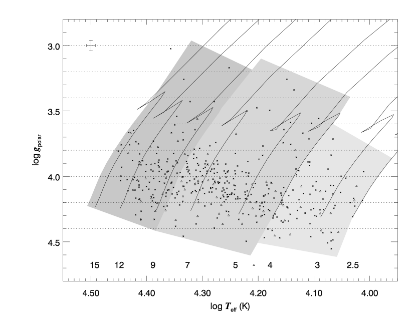
Figure 7: The distribution of the stars in the $\log T_{\rm eff}-\log g_{\rm polar}$ plane. Asterisks are assigned to single stars ($N=325$) while triangles are used for binary systems ($N=78$). The average errors in $\log T_{\rm eff}$ and $\log g_{\rm polar}$ are indicated in the upper-left corner. The solid lines are the evolutionary tracks for non-rotating stellar models (Schaller et al., 1992), marked by the mass ($M_{\odot}$) at the bottom. The three shaded areas outline the three mass groups corresponding to the three panels shown in Figure 10.

Here we examine the changes in the rotational velocity distribution with evolution by considering how these distributions vary with polar gravity. Since our primary goal is to compare the observed distributions with the predictions about stellar rotation evolution for single stars, we need to restrict the numbers of binary systems in our working sample. We began by excluding all stars that have double-line features in their spectra, since these systems have neither reliable $V\sin i$ measurements nor reliable temperature and gravity estimates. We then divided the rest of our sample into two groups, single stars (325 objects) and single-lined binaries (78 objects, identified using the same criterion adopted in the Paper I, $\Delta V_{r}>30$ km s^-1). (Note that we omitted stars from the clusters Tr 14 and Tr 16 because we have only single-night observations for these two and we cannot determine which stars are spectroscopic binaries. We also omitted the O-stars mentioned in §2 because of uncertainties in their derived temperatures and gravities.) The stars in these two groups are plotted in the $\log T_{\rm eff}-\log g_{\rm polar}$ plane in Figure 7 (using asterisks for single stars and triangles for binaries). We also show a set of evolutionary tracks for non-rotating stellar models with masses from 2.5 $M_{\odot}$ to 15 $M_{\odot}$ (Schaller et al., 1992) as indicators of evolutionary status. The current published data on similar evolutionary tracks for rotating stars are restricted to the high mass end of this diagram. However, since the differences between the evolutionary tracks for rotating and non-rotating models are modest except for those cases close to critical rotation, the use of non-rotating stellar evolutionary tracks should be adequate for the statistical analysis that follows. Figure 7 shows that most of the sample stars are located between the ZAMS ($\log g_{\rm polar}=4.3\pm 0.1$) and the TAMS ($\log g_{\rm polar}=3.5\pm 0.1$), and the low mass stars appear to be less evolved. This is the kind of distribution that we would expect for stars selected from young Galactic clusters. There are few targets with unusually large $\log g_{\rm polar}$ that may be double-lined spectroscopic binaries observed at times when line blending makes the H$\gamma$ profile appear very wide. For example, the star with the largest gravity ($\log g_{\rm polar}=4.68$) is NGC 2362 #10008 (= GSC 0654103398), and this target is a radial velocity variable and possible binary (Huang & Gies, 2006).

We show a similar plot for all rapid rotators in our sample ($V\sin i>200$ km s^-1) in Figure 8. These rapid rotators are almost all concentrated in a band close to the ZAMS. This immediately suggests that stars form as rapid rotators and spin down through the MS phase as predicted by the theoretical models. Note that there are three rapid rotators found near the TAMS (from cool to hot, the stars are NGC 7160 #940, NGC 2422 #125, and NGC 457 #128; the latter two are Be stars), and a few more such outliers appear in TAMS region if we lower the boundary on the rapid rotator group to $V\sin i>180$ km s^-1. Why are these three stars separated from all the other rapid rotators? One possibility is that they were born as extremely rapid rotators, so they still have a relatively large amount of angular momentum at the TAMS compared to other stars. However, this argument cannot explain why there is such a clear gap in Figure 8 between these few evolved rapid rotators and the large number of young rapid rotators. Perhaps these stars are examples of those experiencing a spin up during the core contraction that happens near the TAMS. The scarcity of such objects is consistent with the predicted short duration of the spin up phase. They may also be examples of stars spun up by mass transfer in close binaries (Paper I).

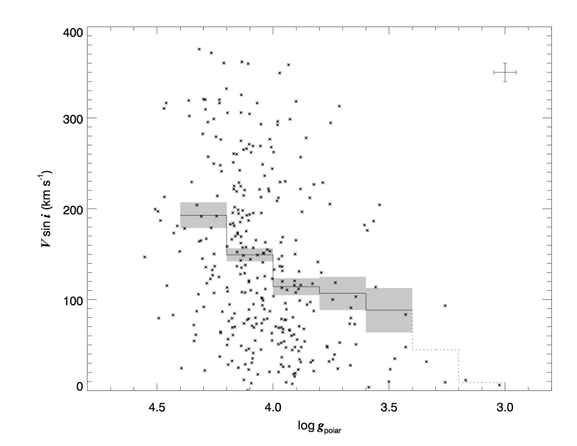
Figure 9: The distribution of the single stars in our sample in the $(\log g_{\rm polar},V\sin i)$ plane. The average errors in $V\sin i$ and $\log g_{\rm polar}$ are plotted in the upper-right corner. The solid line shows the mean $V\sin i$ of each 0.2 dex bin of $\log g_{\rm polar}$ that contains 6 or more measurements while the dotted line shows the same for the rest of bins. The shaded areas enclose the associated error of the mean in each bin.

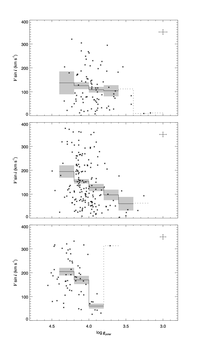
Figure 10: The same $(\log g_{\rm polar},V\sin i)$ distribution as shown in Fig. 9, but here each panel is limited to single stars within a specified mass range. The top panel is for the high mass group ($8.5M_{\odot}<M\leq 16M_{\odot}$, the darkest shaded region in Fig. 7); the middle panel $-$ the middle mass group ($4M_{\odot}<M\leq 8.5M_{\odot}$); the bottom panel $-$ the low mass group ($2.5M_{\odot}<M\leq 4M_{\odot}$, the lightest shaded region in Fig. 7).

We next consider the statistics of the rotational velocity distribution as a function of evolutionary state by plotting diagrams of $V\sin i$ versus $\log g_{\rm polar}$. Figure 9 shows the distribution of the single stars in our sample in the $V\sin i-\log g_{\rm polar}$ plane. These stars were grouped into 0.2 dex bins of $\log g_{\rm polar}$, and the mean and the range within one standard deviation of the mean for each bin are plotted as a solid line and gray-shaded zone, respectively. The mean $V\sin i$ decreases from $193\pm 14$ km s^-1 near the ZAMS to $88\pm 24$ km s^-1 near the TAMS. If we assume that the ratio of $<V>/<V\sin i>=4/\pi$ holds for our sample, then the mean equatorial velocity for B type stars is $246\pm 18$ km s^-1 at ZAMS and $112\pm 31$ km s^-1 at TAMS. This subsample of single stars was further divided into three mass categories (shown by the three shaded areas in Fig. 7): the high mass group (88 stars, $8.5M_{\odot}<M\leq 16M_{\odot}$) is shown in the top panel of Figure 10; the middle mass group (174 stars, $4M_{\odot}<M\leq 8.5M_{\odot}$) in the middle panel, and the low mass group (62 stars, $2.5M_{\odot}<M<4M_{\odot}$) in the bottom panel. All three groups show a spin down trend with decreasing polar gravity, but their slopes differ. The high mass group has a shallow spin down beginning from a relatively small initial mean of $V\sin i=137\pm 48$ km s^-1 (or $<V>=174$ km s^-1). The two bins ($\log g=3.5,3.7$, total 15 stars) around the TAMS still have a relatively high mean $V\sin i$ value, $106\pm 29$ km s^-1 (or $<V>=134$ km s^-1). This group has an average mass of 11 $M_{\odot}$, and it is the only mass range covered by current theoretical studies of rotating stars. The theoretical calculations (Heger & Langer, 2000; Meynet & Maeder, 2000) of the spin down rate agrees with our statistical results for the high mass group. Heger & Langer (2000) show (in their Fig. 10) that a star of mass $12M_{\odot}$ starting with $V=205$ km s^-1 will spin down to 160 km s^-1 at the TAMS. Meynet & Maeder (2000) find a similar result for the same mass model: for $V=200$ km s^-1 at ZAMS, the equatorial velocity declines to 141 km s^-1 at TAMS.

Surprisingly, the middle mass and low mass groups show much steeper spin down slopes (with the interesting exception of the rapid rotator, NGC 7160 #940 = BD$+61^{\circ}2222$, at $\log g_{\rm polar}=3.7$ in the bottom panel of Figure 10). Similar spin down differences among these mass groups were found for the field B-stars by Abt et al. (2002). This difference might imply that an additional angular momentum loss mechanism, perhaps involving magnetic fields, becomes important in these middle and lower mass B-type stars. The presence of low gravity stars in the lower mass groups (summarized in Table 6) is puzzling if they are evolved objects. Our sample is drawn from young clusters (most are younger than $\log{\rm age}=7.4$, except for NGC 2422 with $\log{\rm age}=7.86$; see Paper I), so we would not expect to find any evolved stars among the objects in the middle and lower mass groups. Massey et al. (1995) present HR-diagrams for a number of young clusters, and they find many cases where there are significant numbers of late type B-stars with positions well above the main sequence. They argue that these objects are pre-main sequence stars that have not yet contracted to their main sequence radii. We suspect that many of the low gravity objects shown in the middle and bottom panels of Figure 10 are also pre-main sequence stars. If so, then they will evolve in the future from low to high gravity as they approach the main sequence, and our results would then suggest that they spin up as they do so to conserve angular momentum.

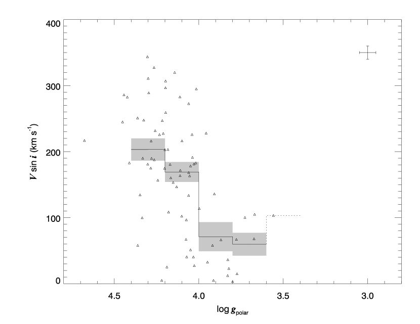
Figure 11: The $(\log g_{\rm polar},V\sin i)$ distribution for probable single-lined binary systems.

Our sample of 78 single-lined binary stars is too small to divide into different mass groups, so we plot them all in one diagram in Figure 11. The binary systems appear to experience more spin down than the single B-stars (compare with Fig. 9). Abt et al. (2002) found that synchronization processes in short-period binary systems can dramatically reduce the rotational velocity of the components. If this is the major reason for the decline in $V\sin i$ in our binary sample, then it appears that tidal synchronization becomes significant in many close binaries when the more massive component attains a polar gravity of $\log g_{\rm polar}=3.9$, i.e., at a point when the star’s larger radius makes the tidal interaction more effective in driving the rotation towards orbital synchronization.

5 Helium Abundance

Rotation influences the shape and temperature of a star’s outer layers, but it also affects a star’s interior structure. Rotation will promote internal mixing processes which cause an exchange of gas between the core and the envelope, so that fresh hydrogen can migrate down to the core and fusion products can be dredged up to the surface. The consequence of this mixing is a gradual abundance change of some elements on surface during the MS phase (He and N become enriched while C and O decrease). The magnitude of the abundance change is predicted to be related to stellar rotational velocity because faster rotation will trigger stronger mixing (Heger & Langer, 2000; Meynet & Maeder, 2000). In this section we present He abundance measurements from our spectra that we analyze for the expected correlations with evolutionary state and rotational velocity.

5.1 Measuring the Helium Abundance

We can obtain a helium abundance by comparing the observed and model profiles provided we have reliable estimates of $T_{\rm eff}$, $\log g$, and the microturbulent velocity $V_{t}$. We already have surface mean values for the first two parameters ($T_{\rm eff}$ and $\log g$) from H$\gamma$ line fitting (§2). We adopted a constant value for the microturbulent velocity, $V_{t}=2$ km s^-1, that is comparable to the value found in multi-line studies of similar field B-stars (Lyubimkov, Rostopchin, & Lambert, 2004). The consequences of this simplification for our He abundance measurements are relatively minor. For example, we calculated the equivalent widths of He I $\lambda\lambda 4026,4387,4471$ using a range of assumed $V_{t}=0-8$ km s^-1 for cases of $T_{\rm eff}=16000$ and 20000 K and $\log g=3.5$ and 4.0. The largest difference in the resulting equivalent width is $\approx 2.5\%$ between $V_{t}=0$ and 8 km s^-1 for the case of the He I $\lambda 4387$ line at $T_{\rm eff}=20000$ K and $\log g=3.5$. These He I strength changes with microturbulent velocity are similar to the case presented by Lyubimkov et al. (2004) for $T_{\rm eff}=25000$ K and $\log g=4.0$. All of these results demonstrate that the changes in equivalent width of He I $\lambda\lambda 4026,4387,4471$ that result from a different choice of $V_{t}$ are small compared to observational errors for MS B-type stars. The $V_{t}$ measurements of field B stars by Lyubimkov et al. (2004) are mainly lower than 8 km s^-1 with a few exceptions of hot and evolved stars, which are rare in our sample. Thus, our assumption of constant $V_{t}=2$ km s^-1 for all the sample stars will have a negligible impact on our derived helium abundances.

The theoretical He I $\lambda\lambda 4026,4387,4471$ profiles were calculated using the SYNSPEC code and Kurucz line blanketed LTE atmosphere models in same way as we did for the H$\gamma$ line (§2) to include rotational and instrumental broadening. We derived five template spectra for each line corresponding to helium abundances of 1/4, 1/2, 1, 2, and 4 times the solar value. We then made a bilinear interpolation in our $(T_{\rm eff},\log g)$ grid to estimate the profiles over the run of He abundance for the specific temperature and gravity of each star. The $\chi^{2}$ residuals of the differences between each of the five template and observed spectra were fitted with a polynomial curve to locate the minimum residual position and hence the He abundance measurement for the particular line. Examples of the fits are illustrated in Figure 12. Generally each star has three abundance measurements from the three He I lines, and these are listed in Table 1 (columns 9 – 11) together with the mean and standard deviation of the He abundance (columns 12 – 13). (All of these abundances include a small correction for non-LTE effects that is described in the next paragraph.) Note that one or more measurements may be missing for some stars due to: (1) line blending in double-lined spectroscopic binaries; (2) excess noise in the spectral regions of interest; (3) severe line blending with nearby metallic transitions; (4) extreme weakness of the He I lines in the cooler stars ($T_{\rm eff}<11500$ K); (5) those few cases where the He abundance appears to be either extremely high ($\gg 4\times$ solar) or low ($\ll 1/4\times$ solar) and beyond the scope of our abundance analysis. We show examples of a He-weak and a He-strong spectrum in Figure 13. These extreme targets are the He-weak stars IC 2395 #98, #122, NGC 2244 #59, #298, and NGC 2362 #73, and the He-strong star NGC 6193 #17.

The He abundances we derive are based on LTE models for H and He which may not be accurate due to neglect of non-LTE effects, especially for hot and more evolved B giant stars ($T_{\rm eff}>25000$ K and $\log g<3.5$). We need to apply some reliable corrections to the abundances to account for these non-LTE effects. The differences in the He line equivalent widths between LTE and non-LTE models were investigated by Auer & Mihalas (1973). However, their work was based on simple atmosphere models without line blanketing, and thus, is not directly applicable for our purposes. Fortunately, we were able to obtain a set of non-LTE, line-blanketed model B-star spectra from T. Lanz and I. Hubeny (Lanz & Hubeny, 2005) that represent an extension of their OSTAR2002 grid (Lanz & Hubeny, 2003). We calculated the equivalent widths for both the LTE (based on Kurucz models) and non-LTE (Lanz & Hubeny) cases (see Table 7), and then used them to derive He abundance ($\epsilon$) corrections based upon stellar temperature and gravity. These corrections are small in most cases ($\Delta\log(\epsilon)<0.1$ dex) and are only significant among the hotter and more evolved stars.

The He abundances derived from each of the three He I lines should lead to a consistent result in principle. However, Lyubimkov et al. (2004) found that line-to-line differences do exist. They showed that the ratio of the equivalent width of He I $\lambda 4026$ to that of He I $\lambda 4471$ decreases with increasing temperature among observed B-stars, while theoretical models predict a constant or increasing ratio between these lines among the hotter stars (and a similar trend exists between the He I $\lambda 4387$ and He I $\lambda 4922$ equivalent widths). The direct consequence of this discrepancy is that the He abundances derived from He I $\lambda\lambda 4471,4922$ are greater than those derived from He I $\lambda\lambda 4026,4387$. The same kind of line-to-line differences are apparently present in our analysis as well. We plot in Figure 14 the derived He abundance ratios $\log[\epsilon(4471)/\epsilon(4026)]$ and $\log[\epsilon(4387)/\epsilon(4026)]$ as a function of $T_{\rm eff}$. The mean value of $\log[\epsilon(4471)/\epsilon(4026)]$ increases from $\approx 0.0$ dex at the cool end to +0.2 dex at $T_{\rm eff}=26000$ K. On the other hand, the differences between the abundance results from He I $\lambda 4026$ and He I $\lambda 4387$ are small except at the cool end where they differ roughly by +0.1 dex (probably caused by line blending effects from the neglected lines of Mg II $\lambda 4384.6,4390.6$ and Fe II $\lambda 4385.4$ that strengthen in the cooler B-stars). Lyubimkov et al. (2004) advocate the use of the He I $\lambda\lambda 4471,4922$ lines based upon their better broadening theory and their consistent results for the helium weak stars. Because our data show similar line-to-line differences, we will focus our attention on the abundance derived from He I $\lambda 4471$, as advocated by Lyubimkov et al. (2004). Since both the individual and mean line abundances are given in Table 1, it is straight forward to analyze the data for any subset of these lines.

We used the standard deviation of the He abundance measurements from He I $\lambda\lambda 4026$, $4387$, $4471$ as a measure of the He abundance error (last column of Table 1), which is adequate for statistical purposes but may underestimate the actual errors in some cases. The mean errors in He abundance are $\pm 0.07$ dex for stars with $T_{\rm eff}\geq 23000$ K, $\pm 0.04$ dex for stars with $23000{\rm~{}K}>T_{\rm eff}\geq 17000$ K, and $\pm 0.05$ dex for stars with $T_{\rm eff}<17000$ K. These error estimates reflect both the noise in the observed spectra and the line-to-line He abundance differences discussed above. The errors in the He abundance due to uncertainties in the derived $T_{\rm eff}$ and $\log g$ values (columns 4 and 6 of Table 1) and due to possible differences in microturbulence from the adopted value are all smaller ($<0.04$ dex) than means listed above.

5.2 Evolution of the Helium Abundance

We plot in Figure 15 our derived He abundances for all the single stars and single-lined binaries in our sample versus $\log g_{\rm polar}$, which we suggest is a good indicator of evolutionary state (§3). The scatter in this figure is both significant (see the error bar in the upper left hand corner) and surprising. There is a concentration of data points near the solar He abundance that shows a possible trend of increasing He abundance with age (and decreasing $\log g_{\rm polar}$), but a large fraction of the measurements are distributed over a wide range in He abundance. Our sample appears to contain a large number of helium peculiar stars, both weak and strong, in striking contrast to the sample analyzed by Lyubimkov et al. (2004) who identified only two helium weak stars out of 102 B0 - B5 field stars. Any evolutionary trend of He abundance that may exist in Figure 15 is lost in the large scatter introduced by the He peculiar stars.

Studies of the helium peculiar stars (Borra & Landstreet, 1979; Borra, Landstreet, & Thompson, 1983) indicate that they are found only among stars of subtype later than B2. This distribution is clearly confirmed in our results. We plot in Figure 16 a diagram of He abundance versus $T_{\rm eff}$, where we see that almost all the He peculiar stars have temperatures $T_{\rm eff}<23000$ K. Below 20000 K (B2) we find that about one third (67 of 199) of the stars have a large He abundance deviation, $|\log(\epsilon/\epsilon_{\odot})|>0.3$ dex, while only 8 of 127 stars above this temperature have such He peculiarities. In fact, in the low temperature range ($T_{\rm eff}<18000$ K), the helium peculiar stars are so pervasive and uniformly distributed in abundance that there are no longer any clear boundaries defining the He-weak, He-normal, and He-strong stars in our sample. The mean observational errors in abundance are much smaller than the observed spread in He abundance seen in Figure 16.

There is much evidence to suggest that both the He-strong and He-weak stars have strong magnetic fields that alter the surface abundance distribution of some chemical species (Mathys, 2004). Indeed there are some helium variable stars, such as HD 125823, that periodically vary between He-weak and He-strong over their rotation cycle (Jaschek et al., 1968). Because of the preponderance of helium peculiar stars among the cooler objects in our sample, we cannot easily differentiate between helium enrichment due to evolutionary effects or due to magnetic effects. Therefore, we will restrict our analysis of evolutionary effects to those stars with $T_{\rm eff}>23000$ K where no He peculiar stars are found. This temperature range corresponds approximately to the high mass group of single stars (88 objects) plotted in the darker shaded region of Figure 7.

The new diagram of He abundance versus $\log g_{\rm polar}$ for the high mass star group ($8.5M_{\odot}<M<16M_{\odot}$) appears in Figure 17. We can clearly see in this figure that the surface helium abundance is gradually enriched as stars evolve from ZAMS ($\log g_{\rm polar}=4.3$) to TAMS ($\log g_{\rm polar}=3.5$). We made a linear least squares fit to the data (shown as a dotted line)

$$\log(\epsilon/\epsilon_{\odot})=(-0.114\pm 0.059)~{}\log g_{\rm polar}~{}+~{}(0.494\pm 0.012)$$

that indicates an average He abundance increase of $0.09\pm 0.05$ dex (or $23\pm 13\%$) between ZAMS ($\log g_{\rm polar}=4.3$) and TAMS ($\log g_{\rm polar}=3.5$). This estimate is in reasonable agreement with the results of Lyubimkov et al. (2004) who found a ZAMS to TAMS increase in He abundance of $26\%$ for stars in the mass range $4-11M_{\odot}$ and $67\%$ for more massive stars in the range $12-19M_{\odot}$.

5.3 Rotational Effects on the Helium Abundance

The theoretical models for mixing in rotating stars predict that the enrichment of surface helium increases with age and with rotation velocity. The faster the stars rotate, the greater will be the He enrichment as stars evolve towards the TAMS. In order to search for a correlation between He abundance and rotation ($V\sin i$), we must again restrict our sample to the hotter, more massive stars to avoid introducing the complexities of the helium peculiar stars (§5.2).

If the He abundance really does depend on both evolutionary state and rotational velocity, then it is important to select subsamples of comparable evolutionary status in order to investigate how the He abundances may vary with rotation. We divided the same high mass group (§5.2) into three subsamples according to their $\log g_{\rm polar}$ values, namely the young subgroup (22 stars, $4.5\geq\log g_{\rm polar}>4.1$), the mid-age subgroup (47 stars, $4.1\geq\log g_{\rm polar}>3.8$), and the old subgroup (14 stars, $3.8\geq\log g_{\rm polar}>3.4$). We plot the distribution of He abundance versus $V\sin i$ for these three subgroups in the three panels of Figure 18. Because each panel contains only stars having similar evolutionary status (with a narrow range in $\log g_{\rm polar}$), the differences in He abundance due to differences in evolutionary state are much reduced. Therefore, any correlation between He abundance and $V\sin i$ found in each panel will reflect mainly the influence of stellar rotation. We made linear least squares fits for each of these subgroups that are also plotted in each panel. The fit results are (from young to old):

$$\log(\epsilon/\epsilon_{\odot})=(-0.0\pm 2.5)\times 10^{-4}~{}V\sin i~{}+~{}(0.043\pm 0.024)$$

$$\log(\epsilon/\epsilon_{\odot})=(0.3\pm 1.6)\times 10^{-4}~{}V\sin i~{}+~{}(0.015\pm 0.013)$$

$$\log(\epsilon/\epsilon_{\odot})=(4.1\pm 2.3)\times 10^{-4}~{}V\sin i~{}+~{}(0.009\pm 0.019)$$

We can see that there is basically no dependence on rotation for the He abundances of the stars in the young and mid-age subgroups. However, there does appear to be a correlation between He abundance and rotation among the stars in the old subgroup. Though there are fewer stars with high $V\sin i$ in the old group (perhaps due to spin down), a positive slope is clearly seen that is larger than that of the younger subgroups.

Our results appear to support the predictions for the evolution of rotating stars, specifically that rotationally induced mixing during the MS results in a He enrichment of the photosphere (Fig. 17) and that the enrichment is greater in stars that spin faster (Fig. 18). The qualitative agreement is gratifying, but it is difficult to make a quantitative comparison with theoretical predictions because our rotation measurements contain the unknown projection factor $\sin i$ and because our samples are relatively small. However, both problems will become less significant as more observations of this kind are made.

6 Conclusions

Our main conclusions can be summarized as follows:

(1) We determined average effective temperatures ($T_{\rm eff}$) and gravities ($\log g$) of 461 OB stars in 19 young clusters (most of which are MS stars) by fitting the H$\gamma$ profile in their spectra. Our numerical tests using realistic models for rotating stars show that the measured $T_{\rm eff}$ and $\log g$ are reliable estimates of the average physical conditions in the photosphere for most of the B-type stars we observed.

(2) We used the profile synthesis results for rotating stars to develop a method to estimate the true polar gravity of a rotating star based upon its measured $T_{\rm eff}$, $\log g$, and $V\sin i$. We argue that $\log g_{\rm polar}$ is a better indicator of the evolutionary status of a rotating star than the average $\log g$ (particularly in the case of rapid rotators).

(3) A statistical analysis of the $V\sin i$ distribution as a function of evolutionary state ($\log g_{\rm polar}$) shows that all these OB stars experience a spin down during the MS phase as theories of rotating stars predict. The spin down behavior of the high mass star group in our sample ($8.5M_{\odot}<M<16M_{\odot}$) quantitatively agrees with theoretical calculations that assume that the spin down is caused by rotationally-aided stellar wind mass loss. We found a few relatively fast rotators among stars nearing the TAMS, and these may be stars spun up by a short core contraction phase or by mass transfer in a close binary. We also found that close binaries generally experience a significant spin down around the stage where $\log g_{\rm polar}=3.9$ that is probably the result of tidal interaction and orbital synchronization.

(4) We determined He abundances for most of the stars through a comparison of the observed and synthetic profiles of He I lines. Our non-LTE corrected data show that the He abundances measured from He I $\lambda 4026$ and from He I $\lambda 4471$ differ by a small amount that increases with the temperature of the star (also found by Lyubimkov et al. 2004).

(5) We were surprised to find that our sample contains many helium peculiar stars (He-weak and He-strong), which are mainly objects with $T_{\rm eff}<23000$ K. In fact, the distribution of He abundances among stars with $T_{\rm eff}<18000$ K is so broad and uniform that it becomes difficult to differentiate between the He-weak, He-normal, and He-strong stars. Unfortunately, this scatter makes impossible an analysis of evolutionary He abundance changes for the cooler stars.

(6) Because of the problems introduced by the large number of helium peculiar stars among the cooler stars, we limited our analysis of evolutionary changes in the He abundance to the high mass stars. We found that the He abundance does increase among stars of more advanced evolutionary state (lower $\log g_{\rm polar}$) and, within groups of common evolutionary state, among stars with larger $V\sin i$. This analysis supports the theoretical claim that rotationally induced mixing plays a key role in the surface He enrichment of rotating stars.

(7) The lower mass stars in our sample have two remarkable properties: relatively low spin rates among the lower gravity stars and a large population of helium peculiar stars. We suggest that both properties may be related to their youth. The lower gravity stars are probably pre-main sequence objects rather than older evolved stars, and they are destined to spin up as they contract and become main sequence stars. Many studies of the helium peculiar stars (Borra & Landstreet, 1979; Borra et al., 1983; Wade et al., 1997; Shore et al., 2004) have concluded that they have strong magnetic fields which cause a non-uniform distribution of helium in the photosphere. We expect that many young B-stars are born with a magnetic field derived from their natal cloud, so the preponderance of helium peculiar stars among the young stars of our sample probably reflects the relatively strong magnetic fields associated with the newborn stars.

Figure 1: The equivalent width of the H$\gamma$ line (including all strong metallic lines in the vicinity) plotted as a function of $T_{\rm eff}$. Each line corresponds to a specific value of $\log g$ that ranges from $\log g=2.6$ (bottom) to $\log g=4.4$ (top) in increments of 0.2 dex. The H$\gamma$ profiles for the intersection points of the curves and the dotted line ($W_{\lambda}=7$ Å) are plotted in Figure 2.

Figure 2: A series of model H$\gamma$ profiles ($V\sin i=150$ km s^-1) with constant equivalent width (7 Å) for a locus of $(T_{\rm eff},\log g)$ points (defined in Fig. 1, $T_{\rm eff}=$ 10666, 11255, 11937, 12778, 13786, 14908, 16300, 17865, 19696, 21897 K for $\log g=$ 2.6, 2.8, $\ldots$, 4.4, respectively). The profiles vary from narrow at low gravity to broad-winged at high gravity due to collisional broadening (linear Stark effect).

Figure 3: The H$\gamma$ line fitting results for the stars (from left to right) NGC 1502 #23 ($T_{\rm eff}=15286\pm 113$ K, $\log g=3.951\pm 0.019$), NGC 869 #803 ($T_{\rm eff}=24838\pm 354$ K, $\log g=3.891\pm 0.033$), and NGC 884 #2255 ($T_{\rm eff}=20360\pm 178$ K, $\log g=3.560\pm 0.022$). The thin solid lines show the fits while the plus signs indicate the observed profiles. The residuals from the fit are shown at the bottom of each plot (offset to 0.2 for clarity).

Figure 4: $\chi^{2}$ residual contour plots for the same stars shown in Fig. 3 (from left to right: NGC 1502 #23, NGC 884 #2255, and NGC 869 #803). The solid lines show contours of increasing error residuals relative to the minimum value (at the center of the contours), while the dotted lines are loci of constant equivalent width (see Fig. 1).

Figure 5: A plot of $T_{\rm eff}$ versus $(B-V)_{0}$ for 441 sample stars. The empirical relationship between stellar effective temperature and intrinsic color is indicated by the solid line (FitzGerald, 1970; Underhill et al., 1979). Those stars marked by letters are NGC 2244 #1254 (A), IC 1805 #1433 (B), NGC 2244 #88 (C), NGC 869 #748 (D), and IC 2944 #105 (E).

Figure 6: A plot of $T_{\rm eff}$ versus spectral subtype for 162 sample stars. The relationship between spectral subtype and effective temperature for OB stars from Böhm-Vitense (1981) is plotted as a solid line. Those stars marked by letters are Tr 16 #23 (A), IC 1805 #118 (B), IC 2944 #48 (C), Tr 16 #20 (D), IC 2944 #110 (E), IC 2944 #102 (F), NGC 869 #847 (G), and NGC 457 #128 (H).

Figure 8: The distribution of the stars with $V\sin i>200$ km s^-1 in the $\log T_{\rm eff}-\log g_{\rm polar}$ plane in the same format as Fig. 7.

Figure 12: Line profile fitting results made to determine the He abundance for the same three stars used in Fig. 3 and 4. Each panel lists the derived LTE He abundance relative to the solar value for He I $\lambda 4026$ (left column), He I $\lambda 4387$ (middle column), and He I $\lambda 4471$ (right column). The stars are (from top to bottom rows) NGC 1502 #23, NGC 869 #803, and NGC 884 #2255.

Figure 13: Top panel: An example of a He-weak star, NGC 1502 #44. The panels from left to right: the He I $\lambda 4026$ region, the H$\gamma$ region, and the He I $\lambda 4471$ region. The solid lines are LTE theoretical profiles synthesized assuming solar abundances and based upon the derived $T_{\rm eff}$, $\log g$, and $V\sin i$ for the star while the dotted lines are LTE theoretical profiles synthesized assuming 1/4 the solar He abundance. Bottom panel: An example of an extreme He-strong star, NGC 6193 #17 (= CD$-48^{\circ}11051$; first noted as a He-rich star by Arnal et al. 1988). The dotted lines are theoretical profiles synthesized assuming 4 times the solar He abundance.

Figure 14: The difference in the non-LTE corrected He abundance from three different He lines plotted against $T_{\rm eff}$. The top panel shows the differences between the results from He I $\lambda 4387$ and He I $\lambda 4026$ and the bottom panel shows the differences between He I $\lambda 4471$ and He I $\lambda 4026$.

Figure 15: A plot of the non-LTE corrected He abundance versus $\log g_{\rm polar}$ for the whole sample. The average measurement errors are indicated in the upper-left corner. Asterisks are assigned to single stars ($N=325$) while triangles are used for binary systems ($N=78$).

Figure 16: A plot of the non-LTE corrected He abundance versus $T_{\rm eff}$ for the whole sample. The average measurement errors are indicated in the upper-left corner. Asterisks are assigned to single stars ($N=325$) while triangles are used for binary systems ($N=78$).

Figure 17: A plot of the non-LTE corrected He abundance versus $\log g_{\rm polar}$ for the high mass group of single stars (see the darker shaded area in Fig. 7). The average measurement errors are indicated in the upper-left corner. The dotted line is the linear least squares fit.

Figure 18: The stars shown in Fig. 17 are divided into three subgroups by their $\log g_{\rm polar}$ values, and plotted in three panels of the non-LTE corrected He abundance versus $V\sin i$. The youngest subgroup is plotted in the top panel while the oldest subgroup is plotted in the bottom panel. The solid lines are the linear least squares fit for each subgroup. The dotted lines are the fits for the younger subgroups replotted in each older group for comparison purposes.

Table 1: Stellar Physical Parameters

Cluster	WEBDA	$T_{\rm eff}$	$\Delta T_{\rm eff}$			$V\sin i$		$\log[{\epsilon\over\epsilon_{\odot}}]$	$\log[{\epsilon\over\epsilon_{\odot}}]$	$\log[{\epsilon\over\epsilon_{\odot}}]$
Name	Index	(K)	(K)	$\log g$	$\Delta\log g$	(km s${}^{-1})$	$\log g_{\rm polar}$	(4026Å)	(4387Å)	(4471Å)	$\overline{\log[{\epsilon\over\epsilon_{\odot}}]}$	$\Delta\log[{\epsilon\over\epsilon_{\odot}}]$
Ber86	01	26878	406	3.84	0.04	185	3.93	$-0.02$	$-0.05$	+0.22	+0.05	0.12
Ber86	12	15440	232	4.05	0.04	309	4.29	$-0.30$	$-0.09$	$-0.39$	$-0.26$	0.12
Ber86	13	28711	191	3.59	0.02	183	3.73	$-0.11$	$-0.19$	+0.26	$-0.02$	0.20
Ber86	15	23049	316	4.10	0.03	023	4.10	+0.04	+0.01	+0.10	+0.05	0.04

Table 2: Photometric Data Sources for Cluster Stars

Cluster	$E(B-V)$
Name	(Loktin et al., 2000)	Sources
NGC 6193	0.475	Herbst & Havlen (1977); Vazquez & Feinstein (1991)
Trumpler 16	0.493	Feinstein (1969); Feinstein, Marraco, & Muzzio (1973); Feinstein (1982);
		Massey & Johnson (1993); Tapia et al. (2003)
IC 1805	0.822	Joshi & Sagar (1983); Massey, Johnson, & DeGioia-Eastwood (1995)
IC 2944	0.320	Thackeray & Wesselink (1965); Ardeberg & Maurice (1977); Pedreros (1984)
Trumpler 14	0.516	Feinstein et al. (1973); Tapia et al. (2003)
NGC 2244	0.463	Johnson (1962); Turner (1976); Ogura & Ishida (1981);
		Perez & Westerlund (1987); Massey et al. (1995)
NGC 2384	0.255	Vogt & Moffat (1972)
NGC 2362	0.095	Johnson & Morgan (1953); Perry (1973)
NGC 3293	0.263	Turner et al. (1980); Herbst & Miller (1982); Baume et al. (2003)
NGC 884	0.560	Tapia et al. (1984); Slesnick, Hillenbrand, & Massey (2002)
NGC 1502	0.759	Dombrowski & Hagen-Thorn (1964); Guetter (1964);
		Purgathofer (1964); Reimann & Pfau (1987)
NGC 869	0.575	Johnson & Morgan (1955); Hiltner (1956); Schild (1965);
		Tapia et al. (1984); Slesnick et al. (2002)
NGC 2467	0.338	Lodén (1966); Feinstein & Vazquez (1989)
Berkeley 86	0.898	Forbes et al. (1992); Massey et al. (1995)
IC 2395	0.066	Claria et al. (2003)
NGC 4755	0.388	Perry et al. (1976); Dachs & Kaiser (1984); Sanner et al. (2001)
NGC 7160	0.375	Hill & Lynas-Gray (1977); Cardon de Lichtbuer (1982); de Graeve (1983)
NGC 457	0.472	Pesch (1959); Hoag et al. (1961); Moffat & Vogt (1974)
NGC 2422	0.070	Lynga (1959); Deutschman, Davis, & Schild (1976); Prisinzano et al. (2003)

Table 3: Physical Parameters of Models

Model	$M$	$R_{\rm polar}$	$T_{\rm polar}$		$V_{c}$
Number	$(M_{\odot})$	$(R_{\odot})$	(K)	$\log g_{\rm polar}$	(km s${}^{-1})$
1	9.5	4.0	25500	4.211	549
2	9.5	5.0	25500	4.018	491
3	9.5	6.4	25500	3.803	434
4	5.5	2.9	18700	4.253	491
5	5.5	3.9	18700	3.996	423
6	5.5	4.9	18700	3.798	378
7	4.0	2.7	15400	4.177	434
8	4.0	3.4	15400	3.977	387
9	4.0	4.1	15400	3.814	352

Table 4: Test Results for Model #1

$i$	$V\sin i$	$T_{msr}$		$T_{geo}$		$T_{flux}$		$T_{L}$
(deg)	(km s-1)	(K)	$\log g_{msr}$	(K)	$\log g_{geo}$	(K)	$\log g_{flux}$	(K)	$\delta\log g$
90	050	25437	4.208	25447	4.208	25446	4.208	25453	0.004
90	100	25282	4.195	25288	4.197	25284	4.197	25312	0.016
90	200	24656	4.143	24635	4.151	24625	4.151	24744	0.068
90	300	23555	4.046	23489	4.068	23487	4.068	23790	0.165
90	400	21927	3.885	21747	3.931	21834	3.938	22462	0.327
70	050	25432	4.207	25443	4.207	25442	4.207	25447	0.004
70	100	25262	4.195	25269	4.196	25267	4.195	25287	0.017
70	200	24562	4.139	24559	4.146	24558	4.146	24644	0.072
70	300	23392	4.044	23314	4.054	23350	4.057	23562	0.167
70	400	21489	3.867	21423	3.902	21661	3.921	22072	0.344
50	050	25407	4.206	25422	4.206	25423	4.206	25420	0.005
50	100	25173	4.191	25188	4.190	25191	4.190	25179	0.020
50	200	24232	4.126	24229	4.122	24267	4.125	24207	0.085
50	300	22549	4.007	22540	3.992	22773	4.010	22586	0.204
30	050	25323	4.203	25341	4.200	25346	4.201	25312	0.008
30	100	24823	4.180	24859	4.167	24888	4.169	24744	0.032
30	200	22631	4.052	22820	4.014	23117	4.037	22462	0.159

Table 5: Polar Gravity Corrections

Model	$V\sin i$	$T_{msr}$
Number	(km s-1)	(K)	$\log g_{msr}$	$\delta\log g$
1	050	25303	4.203	0.009
1	100	24902	4.182	0.029
1	200	23968	4.114	0.098
1	300	23117	4.032	0.180
1	400	21758	3.878	0.333
2	050	25256	4.008	0.011
2	100	24739	3.978	0.040
2	200	23653	3.898	0.120
2	300	22504	3.786	0.232
2	400	20575	3.568	0.449
3	050	25240	3.793	0.011
3	100	24500	3.749	0.054
3	200	23053	3.642	0.161
3	300	21611	3.494	0.309
3	400	18898	3.159	0.644
4	050	18466	4.236	0.018
4	100	18104	4.205	0.048
4	200	17235	4.119	0.135
4	300	16454	4.021	0.232
4	400	15185	3.841	0.412
5	050	18413	3.975	0.021
5	100	17863	3.929	0.067
5	200	16684	3.811	0.185
5	300	15661	3.675	0.321
5	400	13913	3.396	0.600
6	050	18361	3.773	0.024
6	100	17643	3.713	0.085
6	200	16656	3.604	0.194
6	300	15165	3.403	0.395
6	350	14178	3.233	0.565
7	050	15163	4.157	0.020
7	100	14721	4.109	0.069
7	200	14189	4.042	0.135
7	300	13017	3.895	0.282
7	350	12603	3.851	0.326
8	050	15110	3.952	0.025
8	100	14588	3.896	0.081
8	200	13827	3.796	0.181
8	300	12709	3.656	0.321
8	350	12053	3.561	0.416
9	050	15060	3.784	0.030
9	100	14450	3.718	0.096
9	200	13474	3.589	0.225
9	300	12178	3.429	0.385

Table 6: Parameters for Low Gravity Stars in the Middle and Low Mass Groups

Middle Mass Group ($\log g_{\rm polar}<3.6$)				Low Mass Group ($\log g_{\rm polar}<4.0$)
Cluster	WEBDA	$T_{\rm eff}$			Cluster	WEBDA	$T_{\rm eff}$
Name	Index	(kK)	$\log g_{\rm polar}$		Name	Index	(kK)	$\log g_{\rm polar}$
IC2944	00102	14.08	3.26		IC1805	01433	13.41	3.96
NGC869	00768	16.61	3.50		NGC2384	10029	11.73	3.84
NGC2362	10007	15.93	3.48		NGC457	00109	10.25	3.96
NGC2422	00071	13.87	3.59		NGC2244	00088	12.90	3.89
NGC2422	00083	12.72	3.59		NGC2244	00192	13.53	3.99
NGC2467	00016	12.35	3.56		NGC2422	00042	12.83	3.92
NGC2467	00047	13.67	3.34		NGC2467	00002	11.88	3.94
NGC2467	10017	15.11	3.50		NGC2467	00033	12.81	3.89
					NGC7160	00940	11.64	3.71

Table 7: He I Equivalent Widths from Solar Abundance LTE and non-LTE Models

	Non-LTE (Lanz & Hubeny)			LTE (Kurucz)
$T_{\rm eff}$	He I $\lambda 4026$	He I $\lambda 4387$	He I $\lambda 4471$		He I $\lambda 4026$	He I $\lambda 4387$	He I $\lambda 4471$
(K)	(Å)	(Å)	(Å)		(Å)	(Å)	(Å)
$\log g=3.0$
15000	0.772	0.427	0.743		0.828	0.424	0.775
17000	0.883	0.529	0.882		0.903	0.498	0.882
19000	0.831	0.526	0.849		0.828	0.477	0.836
21000	0.706	0.467	0.765		0.676	0.399	0.704
23000	0.605	0.407	0.661		0.526	0.317	0.566
25000	0.531	0.352	0.598		0.378	0.235	0.429
27000	0.474	0.279	0.537		0.209	0.141	0.278
$\log g=4.0$
15000	1.011	0.494	0.863		1.121	0.495	0.941
17000	1.338	0.731	1.201		1.442	0.733	1.250
19000	1.531	0.888	1.393		1.579	0.857	1.411
21000	1.498	0.895	1.385		1.533	0.855	1.395
23000	1.361	0.827	1.261		1.384	0.779	1.268
25000	1.211	0.745	1.147		1.220	0.687	1.120
27000	1.090	0.673	1.050		1.076	0.606	0.994

References

- Abt et al. (2002) Abt, H. A, Levato, H., & Grosso, M. 2002, ApJ, 573, 359
- Ardeberg & Maurice (1977) Ardeberg, A., & Maurice, E. 1977, A&AS, 28, 153
- Arnal et al. (1988) Arnal, M., Morrell, N., Garcia, B., & Levato, H. 1988, PASP, 100, 1076
- Auer & Mihalas (1972) Auer, L. H., & Mihalas, D. 1972, ApJS, 24, 193
- Auer & Mihalas (1973) Auer, L. H., & Mihalas, D. 1973, ApJS, 25, 433
- Baume et al. (2003) Baume, G., Vazquez, R. A., Carraro, G., & Feinstein, A. 2003, A&A, 402, 549
- Böhm-Vitense (1981) Böhm-Vitense, E. 1981, ARA&A, 19, 295
- Borra & Landstreet (1979) Borra, E. F., & Landstreet, J. D. 1979, ApJ, 228, 809
- Borra et al. (1983) Borra, E. F., Landstreet, J. D., & Thompson, I. 1983, ApJS, 53, 151
- Cardon de Lichtbuer (1982) Cardon de Lichtbuer, P. 1982, Vatican Obs. Publ., 2, 1
- Claret (1998) Claret, A. 1998, A&AS, 131, 395
- Claret (2003) Claret, A. 2003, A&A, 406, 623
- Claria et al. (2003) Claria, J. J., Lapasset, E., Piatti, A. E., & Ahumada, A. V. 2003, A&A, 409, 541
- Collins (1963) Collins, G. W., II, 1963, ApJ, 138, 1134
- Collins & Sonneborn (1977) Collins, G. W., II, & Sonneborn, G. H. 1977, ApJS, 34, 41
- Collins et al. (1991) Collins, G. W., II, Truax, R. J., & Cranmer, S. R. 1991, ApJS, 77, 541
- Dachs & Kaiser (1984) Dachs, J., & Kaiser, D. 1984, A&AS, 58, 411
- de Graeve (1983) de Graeve, E. 1983, Vatican Obs. Publ., 2, 31
- Deutschman et al. (1976) Deutschman, W. A., Davis, R. J., & Schild, R. E. 1976, ApJS, 30, 97
- Dombrowski & Hagen-Thorn (1964) Dombrowski, W. A., & Hagen-Thorn, W. A. 1964, Publ. Astron. Obs. Leningrad, 20, 75
- Feinstein (1969) Feinstein, A. 1969, MNRAS, 143, 273
- Feinstein (1982) Feinstein, A. 1982, AJ, 87, 1012
- Feinstein et al. (1973) Feinstein, A., Marraco, H. G., & Muzzio, J. C. 1973, A&AS, 12, 331
- Feinstein & Vazquez (1989) Feinstein, A., & Vazquez, R. A. 1989, A&AS, 77, 321
- FitzGerald (1970) FitzGerald, M. P. 1970, A&A, 4, 234
- Forbes et al. (1992) Forbes, D., English, D., de Robertis, M. M., & Dawson, P. C. 1992, AJ, 103, 916
- Gies & Lambert (1992) Gies, D. R., & Lambert, D. L. 1991, ApJ, 387, 673
- Guetter (1964) Guetter, H. H. 1964, Publ. David Dunlap Obs., 2, 13
- Gummersbach et al. (1998) Gummersbach, C. A., Kaufer, A., Schaefer, D. R., Szeifert, T., & Wolf, B. 1998, A&A, 338, 881
- Heger & Langer (2000) Heger, A., & Langer, N. 2000, ApJ, 544, 1016
- Herbst & Havlen (1977) Herbst, W., & Havlen, R. J. 1977, A&AS, 30, 279
- Herbst & Miller (1982) Herbst, W., & Miller, D. P. 1982, AJ, 87, 1478
- Hill & Lynas-Gray (1977) Hill, P. W., & Lynas-Gray, A. E. 1977, MNRAS, 180, 69
- Hiltner (1956) Hiltner, W. A. 1956, ApJS, 2, 389
- Hoag et al. (1961) Hoag, A. A., Johnson, H. L., Iriarte, B., Mitchell, R. I., & Hallam, K. L. 1961, Publ. USNO Second Ser., 17, 345
- Huang & Gies (2006) Huang, W., & Gies, D. R. 2006, ApJ, submitted (Paper I; astro-ph/0510450)
- Hubeny & Lanz (1995) Hubeny, I., & Lanz, T. 1995, ApJ, 439, 875
- Jackson et al. (2005) Jackson, S., MacGregor, K. B., & Skumanich, A. 2005, ApJS, 156, 245
- Jaschek et al. (1968) Jaschek, C., Jaschek, M., Morgan, W. W., & Slettebak, A. 1968, ApJ, 153, L87
- Johnson (1962) Johnson, H. L. 1962, ApJ, 136, 1135
- Johnson & Morgan (1953) Johnson, H. L., & Morgan, W. W. 1953, ApJ, 117, 313
- Johnson & Morgan (1955) Johnson, H. L., & Morgan, W. W. 1955, ApJ, 122, 429
- Joshi & Sagar (1983) Joshi, U. C., & Sagar, R. 1983, J. RASC, 77, 40
- Lanz & Hubeny (2003) Lanz, T., & Hubeny, I. 2003, ApJS, 146, 417
- Lanz & Hubeny (2005) Lanz, T., & Hubeny, I. 2005, American Astronomical Society Meeting 207 Abstracts, #182.21
- Leone & Manfre (1997) Leone, F., & Manfre, M. 1997, A&A, 320, 257
- Lodén (1966) Lodén, L. O. 1966, Arkiv för Astronomi, 4, 65
- Loktin et al. (2000) Loktin, A.V., Gerasimenko, T.P., & Malysheva, L.K. 2001, Astron. Astrophys. Trans., 20, 607
- Lynga (1959) Lynga, G. 1959, Ark. Astron., 2, 379
- Lyubimkov et al. (2004) Lyubimkov, L. S., Rostopchin, S. I., & Lambert, D. L. 2004, MNRAS, 351, 745
- Massey & Johnson (1993) Massey, P., & Johnson, J. 1993, AJ, 105, 980
- Massey et al. (1995) Massey, P., Johnson, K. E., & DeGioia-Eastwood, K. 1995, ApJ, 454, 151
- Mathys (2004) Mathys, G. 2004, in Stellar Rotation, Proc. IAU Symp. 215, ed. A. Maeder & P. Eenens (San Francisco: ASP), 270
- Mathys et al. (2002) Mathys, G., Andrievsky, S. M., Barbuy, B., Cunha, K., & Korotin, S. A. 2002, A&A, 387, 890
- McAlister et al. (2005) McAlister, H. A., et al. 2005, ApJ, 608, 439
- Mermilliod & Paunzen (2003) Mermilliod, J.-C., & Paunzen, E. 2003, A&A, 410, 511
- Meynet & Maeder (1997) Meynet, G., & Maeder, A. 1997, A&A, 321, 465
- Meynet & Maeder (2000) Meynet, G., & Maeder, A. 2000, A&A, 361, 101
- Moffat & Vogt (1974) Moffat, A. F. J., & Vogt, N. 1974, Veroeff. Astron. Inst. Bochum, 2, 1
- Ogura & Ishida (1981) Ogura, K., & Ishida, K. 1981, Publ. Astron. Soc. Japan, 33, 149
- Pedreros (1984) Pedreros, M. H. 1984, Ph.D. thesis (Univ. Toronto, David Dunlap Obs.)
- Perez & Westerlund (1987) Perez, M. R., & Westerlund, B. E. 1987, PASP, 99, 1050
- Perry (1973) Perry, C. L. 1973, in Spectral Classification and Multicolour Photometry, IAU Symp. 50, ed. C. Fehrenbach & B. E. Westerlund (Dordrecht: Reidel), 192
- Perry et al. (1976) Perry, C. L., Franklin, C. B., Landolt, A. U., & Crawford, D. L. 1976, AJ, 81, 632
- Pesch (1959) Pesch, P. 1959, ApJ, 130, 764
- Prisinzano et al. (2003) Prisinzano, L., Micela, G., Sciortino, S., & Favata, F. 2003, A&A, 404, 927
- Purgathofer (1964) Purgathofer, A. 1964, Ann. Univ. Sternw. Wien, 26, 2
- Reimann & Pfau (1987) Reimann, H.-G., & Pfau, W. 1987, Astron. Nach., 308, 111
- Sackmann & Anand (1970) Sackmann, I.-J., & Anand, S. P. S. 1970, ApJ, 162, 105
- Sanner et al. (2001) Sanner, J., Brunzendorf, J., Will, J.-M., & Geffert, M. 2001, A&A, 369, 511
- Schaller et al. (1992) Schaller, G., Schaerer, D., Meynet, G., & Maeder, A. 1992, A&AS, 96, 269
- Schild (1965) Schild, R. E. 1965, ApJ, 142, 979
- Shore et al. (2004) Shore, S. N., Bohlender, D. A., Bolton, C. T., North, P., & Hill, G. M. 2004, A&A, 421, 203
- Slesnick et al. (2002) Slesnick, C. L., Hillenbrand, L. A., & Massey, P. 2002, ApJ, 576, 880
- Tapia et al. (1984) Tapia, M., Roth, M., Costero, R., & Navarro, S. 1984, Revista Mex. Astron. Astrofis., 9, 65
- Tapia et al. (2003) Tapia, M., Roth, M., Vazquez, R. A., & Feinstein, A. 2003, MNRAS, 339, 44
- Thackeray & Wesselink (1965) Thackeray, A. D, & Wesselink, A. J. 1965, MNRAS, 131, 121
- Turner (1976) Turner, D. G. 1976, ApJ, 210, 65
- Turner et al. (1980) Turner, D. G., Grieve, G. R., Herbst, W., & Harris, W. E. 1980, AJ, 85, 1193
- Underhill et al. (1979) Underhill, A. B., Divan, L., Prevot-Burnichon, M.-L., & Doazan, V. 1979, MNRAS, 189, 601
- Vazquez & Feinstein (1991) Vazquez, R. A., & Feinstein, A. 1991, A&AS, 92, 863
- Vogt & Moffat (1972) Vogt, N., & Moffat, A. F. J. 1972, A&AS, 7, 133
- Wade et al. (1997) Wade, G. A., Bohlender, D. A., Brown, D. N., Elkin, V. G., Landstreet, J. D., & Romanyuk, I. I. 1997, A&A, 320, 172
- von Zeipel (1924) von Zeipel, H. 1924, MNRAS, 84, 665