Anisotropic thermal emission from magnetized neutron stars

The thermal emission from isolated neutron stars is not well understood. The X-ray spectrum is very close to a blackbody but there is a systematic optical excess flux with respect to the extrapolation to low energy of the best blackbody fit. This fact, in combination with the observed pulsations in the X-ray flux, can be explained by anisotropies in the surface temperature distribution. We study the thermal emission from neutron stars with strong magnetic fields $B\geq 10^{13}$ G in order to explain the origin of the anisotropy. We find (numerically) stationary solutions in axial symmetry of the heat transport equations in the neutron star crust and the condensed envelope. The anisotropy in the conductivity tensor is included consistently. The presence of magnetic fields of the expected strength leads to anisotropy in the surface temperature. Models with toroidal components similar to or larger than the poloidal field reproduce qualitatively the observed spectral properties and variability of isolated neutron stars. Our models also predict spectral features at energies between 0.2 and 0.6 keV for $B=10^{13}-10^{14}$.

1 Introduction

Neutron stars (NS) with large magnetic fields ($B\geq 10^{13}$ G), the so-called magnetars, are becoming more and more abundant as new observations reveal phenomena that can only be explained by the action of strong magnetic fields. It is now believed that the small population (4 objects) of soft gamma repeaters (SGRs) are young neutron stars with magnetic fields in the range $\approx 10^{14}-10^{15}$ G. Another subclass of candidates to be magnetars are the anomalous X–ray pulsars (AXPs), whose high X–ray luminosities and fast spindown rates make them different from isolated radio pulsars or from NS in accreting X-ray binaries. The six members of this family (Tiengo et al. 2005; McGarry et al. 2005) exhibit spin periods in the range 5-12 s, and their inferred magnetic fields (from their period derivative) are in the same range as SGRs (see e.g. Woods & Thompson 2005, for a comprehensive review about these two families of magnetar candidates).

A third rare family of NS, the radio-quiet isolated neutron stars among which RX J1856.4-3754 is the first and brightest example (Walter et al. 1996), shares some common features with the standard magnetars (SGR, AXPs): periods clustered in the range 5-10 s., and increasing evidence of large magnetic fields ($>10^{13}$ G). The properties of the seven confirmed members of this family are summarized in Table 1. The most puzzling feature is the apparent optical excess flux (compared to the extrapolation of the best fit to the X-ray emission) observed in several objects, which needs of the existence of large temperature variations over the surface to reconcile the optical and X-ray spectra (Pons et al. 2002). The evidence of anisotropic temperature distribution is also supported by the fact that several of the thermal spectra show clear X-ray pulsations with pulsation amplitudes from 5 to 20 %, while others (RX J1856, RX J1605) have upper limits of 1.3-3% to the maximum pulsation amplitude (Burwitz et al. 2003; van Kerkwijk et al. 2004), which can be explained in terms of different relative orientations between the rotation and magnetic field axis. Thus, it is worth to investigate the influence of strong magnetic field configurations on the temperature distribution, which has been shown to be able to create large anisotropies in neutron star crusts (Geppert et al. 2004), or in the envelope, where further complications due to quantizing effects of the magnetic field or accreted material have been studied in detail (Potekhin et al. 2003). But there is yet another important issue regarding the thermal emission on magnetized neutron stars. Below some critical temperature (depending on the composition and the magnetic field strength), the gaseous layers of highly magnetized neutron stars may undergo a phase transition that turns the gas into liquid or solid state (Lai 2001), which strongly reduces the emissivity from the NS surface compared to the blackbody case (Brinkmann 1980; Turolla et al. 2004; Pérez–Azorín et al. 2005; van Adelsberg et al. 2005).

In this paper our aim is to extend previous works on the anisotropies and thermal emission of magnetized neutron stars (Geppert et al. 2004) in two main ways: by extending to lower density the calculations, within the model of a condensed surface, and exploring the effect of toroidal components of the magnetic field. The generation of toroidal fields in the early stages of a NS life, and its interplay with the poloidal component is a complex problem linked to convective instabilities, turbulent mean–field dynamo (Bonanno et al. 2003) or the Hall instability (Rheinhardt et al. 2004). The magnitude of the toroidal fields is unknown but usually thought to be larger than the poloidal component and, as we discuss in this paper, have interesting observational implications.

This paper is organized as follows: in the next section the plasma properties in magnetic neutron stars are reviewed. In section 3, the magnetic field configurations used in the calculations are described. In section 4, we describe the equations governing the thermal evolution and structure in the presence of large magnetic fields, the numerical code used for the calculations and some tests. The microphysics input is discussed in section 5 and finally, in section 6, we present our results.

Table 1: Properties of isolated neutron stars observed by ROSAT, Chandra, and XMM-Newton Pons et al. (2002); Haberl (2004); Haberl et al. (2005); Kaplan et al. (2003); Kaplan & van Kerkwijk (2005).

Source	kT	$P$	$\dot{P}$	$\tau$	Optical	Optical	Pulsation	Eline	Bdb/Bcyc
	(eV)	(s)	$10^{-12}$ (s s-1)	$10^{6}$yr		excess factor	amplitude	(keV)	1013 G
RX J0420.0$-$5022	45	3.453	$<9$		B$=26.6$	$<12$	0.12	0.329	$<18$/6.6
RX J0720.4$-$3125	85	8.391	$0.07$	0.6-2	B$=26.6$	6	0.11	0.270	2.4/5.2
RX J0806.4$-$4123	96	11.371	$<2$		B$>24$		0.06	$-$	$<14$/?
1RXS J130848.6+212708/RBS1223	95	10.313	$<6$		$28.6$	$<5$	0.18	0.3	?/2-6
RX J1605.3+3249	95	$-$	$-$		B$=27.2$	11-14	$<0.03$	0.46	?/9.5
RX J1856.4$-$3754	60	$-$	$-$	0.5	V$=25.7$	5-7	$<0.02$	$-$	$-$
1RXS J214303.7+065419/RBS1774	101	9.437	$-$		R$>23$		0.04	0.70	?/14

2 Plasma properties in magnetic neutron stars

The transport properties and in general all physical properties of dense matter are strongly affected by the presence of intense magnetic fields. Before discussing in details the microscopical properties of magnetic matter, we begin by reminding some typical definitions and quantities that serve as indicators of the relative importance of the magnetic field.

The pressure in the crust and envelope is dominated by the contribution of the degenerate electrons. Consider an electron gas whose number density is $n_{e}$. In the absence of magnetic field, the Fermi momentum $p_{F}$, or equivalently the wave number $k_{F}=p_{F}/\hbar$ is

$$k_{F}=(3\pi^{2}n_{e})^{1/3}=\left(\frac{3\pi^{2}\rho Z}{Am_{u}}\right)^{1/3}$$ (1)

where $m_{u}$ is the atomic mass unit, and we have assumed that the ions, with atomic number $Z$ and atomic weight $A$, are completely ionized. This assumption allows to relate $n_{e}$ and the density $\rho$, $\rho=\frac{n_{e}}{Z}Am_{u}$. Defining the dimensionless quantity:

$$x_{F}=\frac{\hbar k_{F}}{m_{e}c}=0.010066\left(\frac{\rho Z}{A}\right)^{1/3}\leavevmode\nobreak\ ,$$ (2)

the Fermi energy is $\epsilon_{F}=m_{e}c^{2}\sqrt{1+x_{F}^{2}}$ and the Fermi temperature is $T_{F}=(\epsilon_{F}-m_{e}c^{2})/k_{B}=m_{e}c^{2}(\sqrt{1+x_{F}^{2}}-1)$. If the matter is at temperature $T$, the electrons are degenerate when $T\ll T_{F}$. This condition is fulfilled in the whole NS except for the outermost parts.

The magnetic field affects the properties of all plasma components, specially the electron component. Motion of free electrons perpendicular to the magnetic field is quantized in Landau levels, which produces that the thermal and electrical conductivities (as well as other quantities) exhibit quantum oscillations. These oscillations change the properties of the degenerate electron gas in the limit of strongly quantizing field in which almost all electrons populate the lowest Landau level. The electron cyclotron frequency corresponding to a magnetic field $B$ is given by

$$\omega_{B}=\frac{eB}{m_{e}c},$$ (3)

and the magnetic field will be considered strongly quantizing if the temperature of the electrons is $T\ll T_{B}$ and the density $\rho<\rho_{B}$, where

$$T_{B} = \frac{\hbar\omega_{B}}{k_{B}}\approx 1.34\times 10^{8}\frac{B_{12}}{\sqrt{1+x_{F}^{2}}}\leavevmode\nobreak\ \mbox{K}$$ (4)

$$\rho_{B} = \frac{Am_{u}n_{B}}{Z}\approx 7.045\times 10^{3}\left(\frac{A}{Z}\right)B_{12}^{3/2}\leavevmode\nobreak\ \mbox{g/cm${}^{3}$}$$ (5)

Here $k_{B}$ is the Boltzmann constant and $n_{B}=(eB/\hbar c)^{3/2}/(\pi^{2}\sqrt{2})$ is the electron number density at which the Fermi energy reaches the lowest Landau level. The magnetic field is called weakly quantizing if $T\leq T_{B}$ but $\rho\gtrsim\rho_{B}$. In this case the quantum oscillations are not very pronounced and occur around their classical value. The oscillations disappear for $T\gg T_{B}$ or $\rho\gg\rho_{B}$ and the field can be treated as classical.

Let us turn now to the properties of the ions. In the absence of magnetic field, the physical state of the ions depends on the Coulomb parameter

$$\Gamma=\frac{(Ze)^{2}}{k_{B}Ta_{i}}\approx\frac{0.23\leavevmode\nobreak\ Z^{2}}{T_{6}}\left(\frac{\rho}{A}\right)^{1/3}$$ (6)

where $a_{i}=(3/4\pi n_{i})^{(1/3)}$ is the ion-sphere radius, and $\rho_{6}$ and $T_{6}$ are, respectively, the density and temperature in units of $10^{6}$ g/cm³ and $10^{6}$ K. When $\Gamma<1$ the ions form a Boltzmann gas, when $1\leq\Gamma<175$ their state is a coupled Coulomb liquid, and when $\Gamma\geq 175$ the liquid freezes into a Coulomb lattice. In general, the quantization of the ionic motion will be significant for temperatures lower than the Debye temperature, which is approximately (for ions arranged in a bcc lattice)

$$T_{D}\approx 0.45\frac{\hbar\omega_{p_{i}}}{k_{B}}\approx 3.5\times 10^{3}\left(\frac{Z}{A}\right)\rho^{1/2}\leavevmode\nobreak\ \mbox{K}$$ (7)

and $\omega_{p_{i}}$ is the ion plasma frequency

$$\omega_{p_{i}}=\left(\frac{4\pi Z^{2}e^{2}n_{i}}{m_{i}}\right)^{1/2}.$$ (8)

In presence of strong magnetic fields, the electrons in an atom are confined to the lowest Landau level, the atoms are elongated and with larger binding energy and covalent bonding between them. Therefore, below some critical temperature (depending on the composition and the magnetic field strength), the gaseous layers of highly magnetized neutron stars may undergo a phase transition that turns the gas into liquid or solid state depending on the value of the Coulomb parameter $\Gamma$ (Lai 2001). For typical magnetic field strengths of $10^{13}$ G, a Fe atmosphere will condensate for $T<0.1$ keV while a H atmosphere needs temperatures lower than 0.03 keV to undergo the phase transition to a condensed state. In such a condensed neutron star surface made of nuclei with atomic number $Z$ and atomic weight $A$, the pressure vanishes at a finite density

$$\rho_{s}\approx 560\leavevmode\nobreak\ AZ^{-3/5}B_{12}^{6/5}{\rm g\,cm}^{-3}$$ (9)

where $B_{12}$ is the magnetic field in units of $10^{12}$ G.

In this latter case, matter is in solid state and phonons become an important agent to transport energy. When $T\geq T_{D}$, many thermal phonons are excited in the lattice, and the phonons behave as a classical gas. However, if temperature is low, $T<T_{D}$, phonons behave as a Bose quantum gas and the number of thermal phonons is strongly reduced. Therefore, the Debye temperature $T_{D}$ allows to discriminate the quantum behaviour from the classical one. Another important parameter related to the phonon processes of scattering is the so-called Umklapp temperature, $T_{U}=T_{D}Z^{1/3}e^{2}/(3\hbar v_{F})$, with $v_{F}$ being the Fermi velocity of electrons.

All the previous properties and definitions are visualized and quantified in Fig. 1, where we show, in a phase diagram for neutron star matter, the Fermi temperature ($T_{F}$) and $T_{B}$ (at $B=10^{13}$ G), the Debye temperature ($T_{D}$) and the Umklapp temperature. The central shaded band indicates the region where matter is in the liquid state, according to Eq. (6) and the condition $1\leq\Gamma<175$. The region below that is the solid state ($\Gamma\geq 175$) and the region above that corresponds to the gaseous state ($\Gamma\leq 1$). For reference, we have included two realistic temperature profiles (dot-dashed lines), corresponding to two different core temperatures ($10^{7}$ K and $10^{8}$ K). The dashed lines appearing on the left–lower corner indicate the transitions to different ionization states (25, 20 and 15 free electrons per atom). The outer layers are composed of pure iron ($Z=26$). For $B=10^{13}$ G, Eq. (5) gives $\rho_{B}=5\times 10^{5}$ g/cm³, therefore, the field is strongly quantizing only at low densities, weakly quantizing in most of the envelope and classical in the crust ($T_{B}\leq T$). The zero pressure density as defined by Eq. (9) is $7\times 10^{4}$ g/cm³.

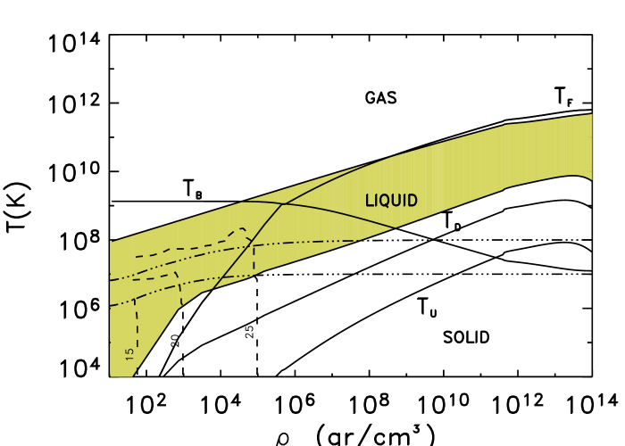
Figure 1: Phase diagram of neutron star matter. The solid lines show the characteristic temperatures $T_{F}$, $T_{B}$, $T_{D}$, and $T_{U}$, where $T_{F}$, $T_{B}$ have been calculated for a magnetic field strength of $B=10^{13}$G. The dashed lines show the domains of partial ionization (at $B=0$). The dot-dashed lines are two realistic temperature profiles for two different models with core temperatures of $10^{8}$ K and $10^{7}$ K.

3 Magnetic field structure.

Although there is robust observational evidence that the external magnetic field is well represented by a dipolar configuration, the internal structure of the magnetic field in neutron stars is unknown, so that one has the freedom to prescribe arbitrary configurations. For weak magnetic fields (magnetic force negligible relative to the pressure gradient or gravity) the deformation of the star is very small and the particular field structure is not important. Finding consistent numerical solutions of the Einstein-Maxwell equations describing the structure of neutron stars endowed with a strong magnetic field, including the effects of the Lorentz force and the curvature of the spacetime induced by the stress-energy tensor of the magnetic field, is a difficult problem only solved for purely poloidal configurations (Bocquet et al. 1995) or very recently including toroidal magnetic fields as perturbations (Ioka & Sasaki 2004). In previous works it has been shown that to obtain a significant deformation of the star magnetic fields of the order of $10^{16}$ G are required. In this work, for simplicity, and partially justified by the fact that most of our models will be force-free (in a Newtonian sense) and less strong ($10^{13}-10^{14}$ G), we will consider a spherical neutron star described by a spherically symmetric metric of the form

$$ds^{2}=-e^{2\Phi(r)}dt^{2}+e^{2\Lambda(r)}dr^{2}+r^{2}(d\theta^{2}+\sin^{2}\theta d\phi^{2})$$ (10)

where $e^{\Phi(r)}$ is the lapse function, $e^{\Lambda}=(1-2m/r)^{-1/2}$ is the space curvature factor, and we have taken $G=c=1$. The usual equation of hydrostatic equilibrium of a relativistic self-gravitating fluid is

$$\frac{dP}{dr}=-(\rho+P)\frac{d\Phi}{dr}\leavevmode\nobreak\ ,$$ (11)

where $P$ is the pressure and $\rho$ is the mass-energy density.

Previous works about the effects of internal magnetic fields restrict the calculations to the simplest models (homogeneous, core dipole, purely radial in a thin layer), mainly to simplify the problem. We address to the review by Tsuruta (1998), (section 5) for an overview of the effects of the magnetic field on the thermal structure and evolution.

However, it is known that neutron stars are born with differential rotation and that convective instabilities play a significant role during the early stages of evolution (Keil et al. 1996; Miralles et al. 2000, 2002). Both differential rotation and convective motions should lead to non-trivial magnetic field structures with non-zero toroidal components (Bonanno et al. 2003), that will evolve according to

$$\frac{\partial\@vec{B}}{\partial t}=-\@vec{\nabla}\times\left(\frac{c^{2}}{4\pi}\hat{R}\cdot\@vec{\nabla}\times\@vec{B}\right)$$ (12)

where we have used the Newtonian equations for simplicity. The relativistic versions of the induction equation for non-rotating and rotating neutron stars can be found in the literature (Geppert et al. 2000; Rezzolla & Ahmedov 2004). Above, $\hat{R}$ is the resistivity tensor.

In the classical (non quantizing) relaxation time approximation, the conductivities are related between them through the magnetization parameter ($\omega_{B}\tau_{0}$) where $\tau_{0}$ is the non-magnetic relaxation time (Urpin & Yakovlev 1980). Then, the magnetic field evolution equation (eq. 12) can be written as follows

$$\frac{\partial\@vec{B}}{\partial t}=-\@vec{\nabla}\times\left(\frac{c^{2}}{4\pi\sigma_{\parallel}}\left(\@vec{\nabla}\times\@vec{B}+\frac{\omega_{B}\tau_{0}}{B}\left(\@vec{\nabla}\times\@vec{B}\right)\times\@vec{B}\right)\right)$$ (13)

with $\sigma_{\parallel}$ being the electrical conductivities parallel to the magnetic field. The first term at the right hand side of the above equation describes Ohmic dissipation and the last term is the Hall-drift, which is not dissipative but affects the current configurations. In general, for strong magnetic fields, $\omega_{B}\tau_{0}\gg 1$, the Hall-drift cannot be neglected. Notice that

$$\frac{c^{2}\omega_{B}\tau_{0}}{4\pi B\sigma_{\parallel}}=\frac{c}{4\pi en_{e}}$$ (14)

which does not depend on the relaxation time, making evident the non-dissipative character of the Hall term. Even if the initial magnetic field is purely poloidal, it will develop a toroidal part during the evolution (Naito & Kojima 1994; Hollerbach & Rüdiger 2004; Rheinhardt et al. 2004; Cumming et al. 2004) and it is necessary to consider how it affects the thermal structure properties of neutron stars. In the remaining of this section we describe the magnetic field configurations used in this work.

3.1 Dipolar magnetic fields

In some previous works, the structure of the magnetic field has been assumed to be poloidal, in which case the field can be conveniently described in terms of the Stokes stream function (Geppert & Urpin 1994; Miralles et al. 1998; Page et al. 2000; Geppert et al. 2004). In spherical coordinates, and writing the $\phi$ component of the vector potential as $A_{\phi}=S(r)\sin\theta/r$, the magnetic field components can be written in terms of the Stoke’s function $S(r)$ as follows

$$B_{r} = \frac{2S(r,t)}{r^{2}}\cos{\theta}$$

$$B_{\theta} = -\frac{\sin{\theta}}{r}\frac{\partial S(r,t)}{\partial r}\leavevmode\nobreak\ .$$ (15)

If we consider the static solution obtained by extending the vacuum solution to the center of the star we have

$$B_{r}=B_{0}R^{3}\frac{\cos{\theta}}{r^{3}}$$

$$B_{\theta}=\frac{B_{0}R^{3}}{2}\frac{\sin{\theta}}{r^{3}}$$ (16)

which corresponds to the choice $S(r)=B_{0}R/r$. This solution diverges at $r=0$. For a magnetic field confined to the crust, $S(r)$ should vanish in the core due to proton superconductivity. In this work we prefer not to restrict ourselves to use poloidal configurations and we use a more general structure as described in the next subsection.

3.2 Force-free magnetic fields

A different, less restrictive, way to prescribe the interior magnetic field is to consider a family of force-free fields. A force-free field is the simplest model for the equilibrium magnetic field in the solar corona, above an active region of sunspots (Low 1993; Wiegelmann & Neukirch 2003). This class of fields are normally used to model the pre-flare coronal configurations and have the advantage to allow large fields and currents to exist simultaneously without exerting any force on the material. This helps to simplify the problem because it allows to use the spherical solution for hydrostatic equilibrium without magnetic fields and because this configurations are not subject to the Hall drift.

A force-free magnetic field obeys

$$\@vec{\nabla}\times\@vec{B}=\mu\@vec{B}$$ (17)

$$\@vec{B}\cdot\@vec{\nabla}\mu=0$$ (18)

where the second equation is a result of the first one and the Maxwell’s equation $\@vec{\nabla}\cdot\@vec{B}=0.$

Let us consider an axially symmetric magnetic configuration. In spherical coordinates, with $(\theta,\phi)$ being the angular coordinates with respect to the magnetic field axis of symmetry, a general magnetic field can be written in terms of the $\phi$ components of the potential vector and the magnetic field as follows:

$$\@vec{B}=\left(\frac{1}{r\sin\theta}\frac{\partial(\sin\theta A_{\phi})}{\partial\theta},-\frac{1}{r}\frac{\partial(rA_{\phi})}{\partial r},B_{\phi}\right)$$ (19)

Therefore, Eq. (17) reads:

$$\left(\frac{\sin\theta}{r}\frac{\partial(\sin\theta B_{\phi})}{\partial\theta},-\frac{1}{r}\frac{\partial(rB_{\phi})}{\partial r},\frac{1}{r}\left(\frac{\partial(rB_{\theta})}{\partial r}-\frac{\partial B_{r}}{\partial\theta}\right)\right)$$

$$=\mu\left(\frac{\sin\theta}{r}\frac{\partial(\sin\theta A_{\phi})}{\partial\theta},-\frac{1}{r}\frac{\partial(rA_{\phi})}{\partial r},B_{\phi}\right).$$ (20)

For simplicity, we will consider solutions with $\mu=$constant, so that Eq. (18) is automatically satisfied, although more general solutions exist. The equality of the $r,\theta$ components in Eq. (20) is obviously satisfied if we take $B_{\phi}=\mu A_{\phi}$. By analogy with the core dipole, we try the ansatz $A_{\phi}=\sin\theta\leavevmode\nobreak\ A(r)$, which leads to the following equation for the $\phi$ components of Eq. (20)

$$\frac{d^{2}A(r)}{dr^{2}}+\frac{2}{r}\frac{dA(r)}{dr}+\left(\mu^{2}-\frac{2}{r^{2}}\right)A(r)=0\leavevmode\nobreak\ .$$ (21)

This is a form of the Riccati-Bessel equation for $l=1$, which has solutions of the form

$$A(r)=aj_{l}(x)+bn_{l}(x)$$ (22)

where $a$,$b$ are constants, $x=\mu r$ and $j_{l}(x)$ and $n_{l}(x)$ are spherical Bessel functions of the first and second kinds. For $l=1$ we have, explicitly:

$$j_{1}(x) = \frac{\sin{x}}{x^{2}}-\frac{\cos{x}}{x}\leavevmode\nobreak\ ,$$

$$n_{1}(x) = -\frac{\cos{x}}{x^{2}}-\frac{\sin{x}}{x}\leavevmode\nobreak\ .$$ (23)

The spherical Bessel functions of the first kind are regular in the origin ($j_{l}(x)\propto x^{l}$), while the functions of the second kind diverge as $n_{l}(x)\propto x^{-(l+1)}$.

Hence, a general interior solution that matches (continuity of the normal component of the magnetic field) with the vacuum dipolar solution at the surface is

$$\@vec{B}=C\left(2\frac{\cos\theta}{r}A(r),-\frac{\sin\theta}{r}\frac{\partial(rA(r))}{\partial r},\mu{\sin\theta}A(r)\right)$$ (24)

where $C=\frac{R_{S}B_{0}}{2A(R_{S})}$ and $B_{0}$ is the value of the magnetic field at the pole. This magnetic field can be obtained from the following potential vector

$$\@vec{A}=C\left(\mu r\leavevmode\nobreak\ {\cos\theta}\leavevmode\nobreak\ A(r),\leavevmode\nobreak\ 0,{\sin\theta}\leavevmode\nobreak\ A(r)\right)$$ (25)

Notice that this general solution includes all simple configurations as particular limits. The core dipole can be recovered by taking the limit $\mu\rightarrow 0$ and considering only the $n_{1}(x)$ functions ($a=0$ in Eq. 22). Alternatively, in the limit $\mu\rightarrow 0$ but considering only the family of regular solutions $j_{1}(x)$, we arrive to the homogeneous magnetic field. In both cases, the $B_{\phi}$ component vanishes. We can also find solutions that match continuously with the two components of the exterior dipole by setting, $l=1$, $a=\cos(\mu R_{S})$, and $b=\sin(\mu R_{S})$. The family of solutions is parametrized by the value of $\mu$, which can be interpreted as a wavenumber. If we want to build crustal magnetic fields that match with an external dipole we only need to adjust the wavenumber to have a vanishing radial component in the crust-core interface ($r=R_{\rm int}$) and continuity of $B_{r}$ and $B_{\theta}$ at the surface ($r=R_{S}$). These values of $\mu$ are the solutions of

$$\tan\left(\mu\left(R_{\rm int}-R_{S}\right)\right)=\mu R_{\rm int}\leavevmode\nobreak\ .$$ (26)

In Fig. 2 we show three examples of crustal magnetic fields for the first three solutions of Eq. (26) with $R_{\rm int}=9.2$ km and $R_{S}=12.247$ km.

In principle there are more solutions of Eq. (20) than the linear one ($B_{\phi}=\mu A_{\phi}$) that we have adopted. A more general discussion about force-free configurations can be found in the literature (Low 1993; Wiegelmann & Neukirch 2003).

Finally, we also want to mention that this general force-free solution can be readily extended to higher order multipoles (i.e. quadrupole). This can be done by replacing in Eq. (24) $\cos\theta$ and $\sin\theta$ by the corresponding Legendre polynomial and its derivative, and using the spherical Bessel functions of the same index $l$. Another advantage of this force-free solution is that, for constant electrical resistivity (although in a realistic NS this approximation is not appropriate), one can readily estimate the diffusion time. The evolution equation (13) is simplified to

$$\frac{\partial\@vec{B}}{\partial t}=-\frac{1}{\tau_{\rm diff}}\@vec{B}$$ (27)

which solution reads

$$\@vec{B}=\@vec{B}_{0}\leavevmode\nobreak\ e^{-t/\tau_{\rm diff}}\leavevmode\nobreak\ .$$ (28)

Here, $\@vec{B}_{0}$ is the initial magnetic field and the decay time is $\tau_{\rm diff}=\frac{4\pi\sigma_{\parallel}}{c^{2}\mu^{2}}$, that for typical conditions in young neutron stars is $10^{6}-10^{7}$ years.

Figure 2: Projections of the field lines on the $(r,\theta)$ plane for force-free magnetic field configurations confined in the region between $R_{int}=9.2$ km and $R_{S}=12.247$ km. From left to right $\mu=0.577,1.569,2.591$ km^-1. All configurations match continuously to an external dipole.

4 Thermal diffusion in highly magnetized neutron stars

4.1 Equations.

For very slowly rotating NSs, and neglecting the magnetic force (which vanishes for force-free fields) the thermal evolution of neutron stars can still be described by the energy balance equation

$$C_{v}e^{\Phi(r)}\frac{\partial T}{\partial t}+\@vec{\nabla}\cdot(e^{2\Phi(r)}\@vec{F})=e^{2\Phi(r)}\dot{\epsilon}$$ (29)

where $C_{v}$ is the specific heat (per unit volume), $\@vec{F}$ is the energy flux and the source term ($\dot{\epsilon}$) includes all energy losses and sources (neutrino emission, frictional or accretion heating, etc). The evolution equation can also be written in integral form applying Gauss’ theorem

$$\int_{V}e^{\Phi(r)}C_{v}\frac{\partial T}{\partial t}dV+\oint_{S}e^{2\Phi(r)}\@vec{F}\cdot d\@vec{S}=\int_{V}e^{2\Phi(r)}\dot{\epsilon}dV$$ (30)

In the diffusion limit, the energy flux is given by

$$e^{\Phi(r)}\@vec{F}=-\hat{\kappa}\cdot\@vec{\nabla}(e^{\Phi(r)}T)$$ (31)

where $\hat{\kappa}$ is the thermal conductivity tensor. Defining a new variable $\tilde{T}=e^{\Phi(r)}T$, the components of the flux can be written as follows

$$e^{\Phi(r)}F_{r}=-(\kappa_{rr}e^{-\Lambda}\partial_{r}\tilde{T}+\frac{\kappa_{r\theta}}{r}\partial_{\theta}\tilde{T})$$

$$e^{\Phi(r)}F_{\theta}=-(\kappa_{\theta r}e^{-\Lambda}\partial_{r}\tilde{T}+\frac{\kappa_{\theta\theta}}{r}\partial_{\theta}\tilde{T})$$ (32)

where $\kappa_{ij}$ are the components of the thermal conductivity tensor. The $\phi$ component of the flux is not considered because we assume axial symmetry.

In the presence of strong magnetic fields, the thermal conductivities are different in the directions parallel and perpendicular to the magnetic field. In the classical relaxation time approximation, and considering that only electrons carry heat, the ratio between the parallel and perpendicular conductivities is related to the magnetization parameter ($\omega_{B}\tau_{0}$) as follows (Urpin & Yakovlev 1980)

$$\frac{\kappa_{\parallel}}{\kappa_{\perp}}=1+(\omega_{B}\tau_{0})^{2}\leavevmode\nobreak\ .$$ (33)

The heat conductivity tensor in spherical coordinates and with the polar axis coinciding with the axis of symmetry of the magnetic field can be written as follows

$$\hat{\kappa} =\kappa_{\perp}\times$$ (40)

$$\left(I+(\omega_{B}\tau_{0})^{2}\left(\begin{array}[]{ccc}b_{r}^{2}&b_{r}b_{\theta}&b_{r}b_{\phi}\\ b_{r}b_{\theta}&b_{\theta}^{2}&b_{\theta}b_{\phi}\\ b_{r}b_{\phi}&b_{\theta}b_{\phi}&b_{\phi}^{2}\\ \end{array}\right)+\omega_{B}\tau_{0}\left(\begin{array}[]{ccc}0&b_{\phi}&-b_{\theta}\\ -b_{\phi}&0&b_{r}\\ b_{\theta}&-b_{r}&0\end{array}\right)\right)$$

where $I$ is the identity matrix and $b_{r},b_{\theta},b_{\phi}$ are the components of the unit vector in the direction of the magnetic field.

With the above expression for $\hat{\kappa}$, the flux reads

$$e^{\Phi(r)}\@vec{F}=-\kappa_{\perp}\left[\@vec{\nabla}\tilde{T}+\left(\omega_{B}\tau_{0}\right)^{2}\left(\@vec{b}\cdot\@vec{\nabla}\tilde{T}\right)\cdot\@vec{b}+\omega_{B}\tau_{0}\left(\@vec{b}\times\@vec{\nabla}\tilde{T}\right)\right]$$ (42)

The Hall contribution to the heat flux is given by the last term on the right hand side of Eq. (42). If the magnetic field geometry has only poloidal components, and the temperature distribution does not depend on the azimuthal angle, $\phi$, the divergence of the Hall term vanishes (Geppert et al. 2004) and it does not affect the energy balance equation (29). However, for a magnetic field structure with a toroidal component, this term contributes to the heat flux, even in axial symmetry. In the following, to simplify notation, we will omit the tilde over the temperature and we will use the symbol $T$ for the red-shifted temperature.

4.2 Boundary conditions.

Boundary conditions can be imposed in either the temperature or the flux in the boundaries of our numerical domain. Only a few years after birth the inner core of a NS becomes isothermal, therefore, in the core-crust interface ($r=R_{int}$) we will impose a fixed core temperature ($T_{c}$). At the surface we impose

$$F(B,T,\theta_{B})=\alpha(B,T,\theta_{B})\sigma T^{4}$$ (43)

where $\sigma$ is the the Stephan-Boltzmann constant and $\alpha(B,T,\theta_{B})$ is the integrated emissivity that depends on the particular model, and $\theta_{B}$ is the angle between the magnetic field and the direction normal to the surface element. At the temperatures of interest and for magnetic fields intense enough to produce the condensation of the gaseous layers, the emissivity at low energies is strongly reduced compared to the blackbody case and depends on the orientation angle (Brinkmann 1980; Turolla et al. 2004; Pérez–Azorín et al. 2005; van Adelsberg et al. 2005).

In Fig. 3 we show the flux factor with (left) and without (right) taking into account the effect of the motion of ions for a dipolar magnetic field of $B_{0}=5\times 10^{13}G$. Based on our previous results (Pérez–Azorín et al. 2005), we have obtained a polynomial fit of $\alpha(B,T,\theta_{B})$ as a function of $T_{6}$ (temperature in units of $10^{6}$ K) and $\cos(\theta_{B})$ for different magnetic field strengths (relative error $<2\%$) with the following form:

$$\alpha=\sum_{i=1}^{6}\sum_{j=1}^{6}a_{i,j}T_{6}^{i-1}\cos^{j-1}(\theta_{B})$$ (44)

The $a_{i,j}$ coefficients for $B=10^{13}$ G and $5\times 10^{13}$ G with and without taking into account the effect of the motion of ions are presented in tables (4–7). The case of isotropic emission (black body) can be recovered by setting $\alpha=1$.

Figure 3: Flux factor $\alpha$ as defined in Eq. (43) for a dipolar magnetic field with $B_{p}=5\times 10^{13}G$, with (left panel) and without (right panel) taking into account the effect of the motion of the ions (considered as free particles).

4.3 Numerical test.

The numerical algorithm consists of a standard finite difference scheme fully implicit in time. The temperature is cell-centered, while the fluxes are calculated at each cell-edge. In order to test the code, we have studied the evolution of a thermal pulse in an infinite medium (neglecting all general relativistic effects), embedded in a homogeneous magnetic field oriented along the z-axis. If the conductivity is constant in the medium, an analytical solution for the temperature profile at a time $t$ is the following:

$$T(\@vec{r},t)=T_{0}{\left(\frac{t_{0}}{t}\right)}^{3/2}\exp{\left[-\frac{r^{2}}{4\kappa_{\perp}t}\left(\sin^{2}\theta+\frac{\cos^{2}\theta}{1+(\omega_{B}\tau_{0})^{2}}\right)\right]}$$ (45)

where $T_{0}$ is a constant (the central temperature at the initial time, $t_{0}$), $\kappa_{\perp}$ is the transverse conductivity and $(\omega_{B}\tau_{0})$ is the magnetization parameter. To check the accuracy of the method, we have compared the numerical evolution of the pulse with the analytical solution, for different values of the parameters $\kappa_{\perp}$ and $\omega_{B}\tau_{0}$. As boundary conditions, we prescribe the temperature corresponding to the analytical solution in the surface and we impose $\@vec{F}=0$ at the center. In Fig. 4 we show the comparison between the analytical (solid) and numerical (stars) solution and for a model with $\omega_{B}\tau_{0}=3$ and $\kappa_{\perp}=10^{2}$ (a.u). The grid resolution is 100$\times$40 (radial$\times$angular). The deviations from the analytical solution in all cases studied are less than $0.1\%$.

Figure 4: Temperature profiles at different times comparing the analytic solution (solid) and the numerical evolution (stars) of a thermal pulse in a medium embedded in a homogeneous magnetic field. For clarity, in the numerical solution we have shown only one out of every six grid points. The parameters of the simulation are $\omega_{B}\tau_{0}=3$ and $\kappa_{\perp}=10^{2}$ (a.u), $t_{0}=10^{-4}$. The left panel shows the evolution of polar profiles and the right panel corresponds to equatorial profiles.

5 Microphysics input.

The microphysical ingredients that enter in the transport equations (29) and (31) are the specific heat and the thermal conductivity. Strictly speaking, the specific heat is not needed to obtain stationary configurations, but we have chosen to evolve Eq. (29) without sources with a fixed inner temperature until the stationary solution is reached. Therefore, by using realistic microphysics input we will obtain also information about the thermal relaxation timescales.

The dominant contribution to the specific heat is that from electrons and ions. For electrons we use the formulae corresponding to a relativistic degenerate Fermi gas while for ions we follow van Riper (1991). The most important ingredient is, however, the thermal conductivity, which has contribution from electron, photon and phonon transport. In this section we summarize the expressions used in the simulations.

5.1 Thermal conductivity.

The region of interest covers a large range of densities, from the core-crust boundary ($\approx 10^{14}$ g/cm³) to the surface, which is given by Eq. (9) in the models of condensed atmosphere. The total conductivity includes the contributions of three carriers,

$$\kappa=\kappa_{e}+\kappa_{rad}+\kappa_{ph}$$ (46)

where $\kappa_{e}$ is the electron conductivity, $\kappa_{rad}$ is the radiative (photon) conductivity and $\kappa_{ph}$ is the phonon conductivity. In non magnetic neutron stars, heat is transported mainly by electrons in the crust and in the inner envelope and by photons near the surface, while the phonon transport is negligible. However, in the presence of strong magnetic fields, this situation may change. While for the transport along the magnetic field the phonon contribution is still negligible, in the transverse direction the electron transport is drastically suppressed, and the phonon contribution may become the most important one. Let us consider each of this contributions separately.

5.1.1 Electron transport

In the crust and the envelope of a neutron star the transport properties are mainly determined by the process of electron scattering off strongly correlated ions. The study of the transport properties of Coulomb plasmas with and without magnetic fields has been a focus of attention for decades (e.g. Flowers & Itoh 1976; Urpin & Yakovlev 1980; Kaminker & Yakovlev 1981; Itoh et al. 1984). For the envelope, we will use the expressions obtained by Potekhin (1999), who calculated the thermal and electrical conductivities of degenerate electrons in magnetized envelopes by means of an effective scattering potential that takes into account multiphonon processes in Coulomb crystals and an appropriate structure factor of ions in Coulomb liquids. For the crust, the practical expression derived by Potekhin (1999) have been later generalized (Gnedin et al. 2001) by including how the size and shape of nuclear charge affects the transport properties as well as reconsidering the electron-phonon scattering processes.

In our calculations we are using the results from Potekhin (1999), whose code is of public domain . For pedagogical purposes, in order to make evident the effect of a large magnetization parameter, we now summarize the classical relations for degenerated electrons. Schematically, the thermal conductivity can be written in terms of some effective relaxation time, $\tau_{ij}$, as follows

$$\kappa_{ij} = \frac{\pi^{2}k_{B}^{2}n_{e}c^{2}T}{3\epsilon_{F}}\tau_{ij}(\epsilon_{F}),$$ (47)

where $\tau_{ij}$ are interpreted as inverse effective collision frequencies. In the non-quantizing case, we can write explicitly the different components in terms of the magnetization parameter ($\omega_{B}\tau_{0}$)

$$\tau_{zz}=\tau_{0},\,\tau_{xx}=\frac{\tau_{0}}{1+\omega_{B}\tau_{0}},\,\tau_{yx}=\frac{\omega_{B}\tau_{0}^{2}}{1+\omega_{B}\tau_{0}}$$ (48)

The three main electron scattering processes that play a role in our scenario are scattering off ions, electron-phonon scattering and scattering off impurities. Semi-analytic expressions and fitting formulae for the relaxation times and thermal conductivities along the magnetic field for all three processes were derived by Potekhin & Yakovlev (1996). The total contribution of electrons to the thermal conductivity is then calculated as

$$\kappa_{e}=\left(\kappa_{e-ph}^{-1}+\kappa_{e-imp}^{-1}\right)^{-1}\leavevmode\nobreak\ .$$ (49)

Figure 5: Magnetization parameter ($\omega_{B}\tau_{0}$) against density for different temperatures (from top to bottom $10^{5}$,$10^{6}$,$10^{7}$,$10^{8}$ K) and $B=10^{13}$G. The solid lines are calculated with an impurity parameter of $Q=0.1$, the dashed lines are for homogeneous matter ($Q=0$) and the dot-dashed lines correspond to highly inhomogeneous matter $Q=10$.

In Fig. 5 we show the magnetization parameter, related to the anisotropy of the thermal conductivity by Eq. (33), as a function of density and for different temperatures. For comparison, we show results with different impurity concentration parameter $Q={n_{\rm imp}(Z_{\rm imp}-Z)^{2}}/{n_{i}}$. The dashed, solid, and dash-dotted lines correspond to $Q=0,0.1$, and 10, respectively. For highly inhomogeneous matter ($Q=10$), the magnetization parameter is strongly reduced in the crust ($\omega_{B}\tau_{0}\approx 1$).

At large temperature the total electron conductivity is weakly dependent on temperature. If the temperature drops below the Umklapp temperature ($T\ll T_{U}$), the Umklapp processes are disallowed and $\kappa\propto T^{-4}$. Therefore, at high temperature the dominant process is the electron-phonon scattering but at low temperature the scattering off impurities becomes the dominant contribution.

5.1.2 Photon transport

Radiative conduction becomes the most effective transport mechanism in the outermost layers of the envelope, where electrons are non degenerate. We employ the expressions derived by Potekhin & Yakovlev (2001) for fully ionized iron, who fitted previous results (Silant’ev & Yakovlev 1980).

Free-free transitions and Thompson scattering off free electrons are the two contributions to the total radiative conductivity, that is calculated according to

$$\kappa_{rad}=\left(\kappa^{-1}_{ff}+\kappa^{-1}_{T}\right)^{-1}$$ (50)

For temperatures below $10^{7}$ K, the dominant contribution comes from free-free transitions, which scales as $\approx\rho^{-2}T^{6.5}$. Notice that for $T<10^{7}$ K we have $\kappa_{\perp}\approx 2\kappa_{\parallel}$.

5.1.3 Phonon transport

Energy transport by phonons is usually orders of magnitude less effective than the usual electron or radiative transport. However, in the situation that we are studying, the large anisotropy induced by the magnetic field can suppress electron thermal conduction in the perpendicular direction by factors of $10^{3}-10^{6}$. Under this circumstances, transport by phonons become important, since this processes will become the most effective way to transport energy in the perpendicular direction. For this reason, we need to include it in our calculations.

Figure 6: Thermal conductivity due to electron transport (dashed line), phonon transport (dot dashed line), photon transport (double dot dashed) and total (continuous line). The left panels show the conductivity in the direction longitudinal to the magnetic field while the right panels show the transverse conductivity, which is strongly suppressed.

In a first approximation, we consider a very simplified model, in which the phonon distribution is characterized by a Debye spectrum and all the relaxation times are functions of the wave vector of one mode only. In this approximation, the lattice thermal conductivity can be expressed as

$$\kappa_{ph}=\frac{k_{B}}{2\pi^{2}c_{s}}\left(\frac{k_{B}}{\hbar}\right)^{3}T^{3}\int_{0}^{T_{D}/T}\tau(x)\frac{x^{4}\exp{(x)}}{(\exp{(x)}-1)^{2}}dx$$ (51)

where $c_{s}$ is the sound speed, $T_{D}$ is the Debye temperature, $x$ is a dimensionless variable ($x\equiv\hbar\omega/k_{B}T$) and $\tau$ is the combined relaxation time, whose reciprocal is the sum of the reciprocal relaxation times for all scattering processes considered, Umklapp and impurity scattering processes (both dissipative) and the three phonon normal scattering which are non dissipative (Holland 1963; Konstantinov et al. 2003):

$$\tau^{-1}=\tau_{U}^{-1}+\tau_{I}^{-1}+\tau_{N}^{-1}$$ (52)

At temperatures $T>T_{D}$, the lattice conductivity is mainly determined by the Umklapp processes, and the integral (51) can be approximated to the expression

$$\kappa_{ph}\sim\frac{\rho c_{s}^{3}a}{4T}$$ (53)

where $a\approx\left(\frac{Am_{B}}{\rho}\right)^{1/3}$ is the lattice constant. At lower temperatures ($T<T_{D}$), dissipative processes make the conductivity to increase very rapidly and the inclusion of impurity and normal phonon scattering becomes necessary. These processes (which conserve the total momentum) cannot by themselves lead to a finite thermal conductivity, but do not allow very large heat currents to be carried by modes of long wavelength. In this low temperature limit the thermal conductivity can be expressed in the form (Callaway 1961)

$$\kappa_{ph}=\frac{k_{B}}{2\pi^{2}c_{s}}\left(\frac{k_{B}}{\hbar}\right)^{3}T^{3}\frac{\left(\int_{0}^{T_{D}/T}x^{4}\exp{(x)}(\exp{(x)}-1)^{-2}dx\right)^{2}}{\int_{0}^{T_{D}/T}\tau_{D}^{-1}x^{4}\exp{(x)}(\exp{(x)}-1)^{-2}dx}$$ (54)

where $\tau_{D}^{-1}=\tau_{U}^{-1}+\tau_{I}^{-1}$. In the limit $\tau_{U}^{-1}=0$ we recover the Ziman limit (Ziman 1971)

$$\kappa_{ph}=\frac{2\hbar\omega_{D}^{3}}{360\pi^{3}c_{s}T\Gamma_{\rm imp}}$$ (55)

where $\omega_{D}$ is the Debye frequency and $\Gamma_{\rm imp}$ is a parameter that takes into account the different atomic masses of the impurities and the lattice deformation.

According to this expressions, in the crust and inner envelope, the heat transport along the magnetic field is dominated by the electron component, while phonons become the main transport agent in the transverse direction (see Fig. 6). If the core temperature is low enough ($T<10^{5}$K), the phonon contribution becomes very important also in the parallel direction, making the crust to be quasi isothermal. Near the surface, the radiative conductivity dominates in both directions.

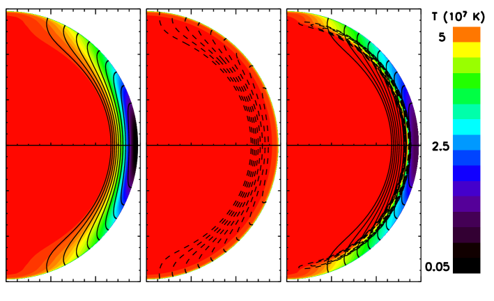
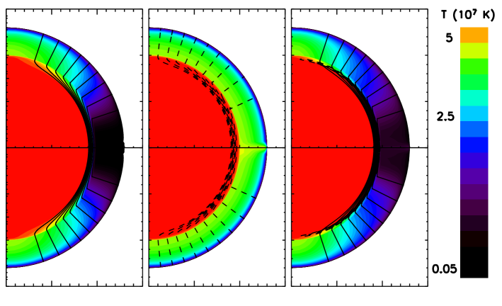
Figure 7: Upper panel: Temperature distribution in the crust of neutron stars with different toroidal components. The poloidal component is the same in all models ($B_{p}=10^{13}$ G) and it is confined to the crust (solid lines). The left panel shows results for a purely poloidal field, the central panel a force-free configuration, and the right panel corresponds to a toroidal component confined to a narrow region of the crust. In the two latter cases the dashed lines show contours of constant $B_{\phi}$. The scale has been stretched about a factor 2 to enlarge the crustal region. Lower panel: Same as the upper panel but stretching the scale to enlarge the region of the envelope.

6 Results.

Our aim is to find stationary solutions of the temperature distribution in a given background magnetic field configuration. We assume that the inner core is isothermal, and that the diffusion time of the magnetic field ($\tau_{\rm diff}$) is much longer than the relaxation time to reach thermal equilibrium so that the magnetic field is kept fixed. We also assume that the sources or sinks of energy (if any) are effective only at longer timescales. This assumptions are justified because both the magnetic diffusion time (either Ohmic or ambipolar) and the cooling time are $>10^{5}$ years, while the typical time to achieve the stationary solution (starting from a constant temperature profile) is $\approx 10^{3}$ years. Notice that the diffusion timescale when the Hall instability occurs is about $10^{4}$ years, so that in this case one would need to consider the coupled evolution of the temperature and the magnetic fields. Instead of solving the equation $\@vec{\nabla}\cdot\@vec{F}=0$ directly, we evolve Eq. (29), without sources, until the stationary solution is reached.

The main effect of the magnetic field on the temperature distribution can be guessed by looking at the expression of the heat flux (42). When the magnetization parameter is large ($\omega_{B}\tau_{0}\gg 1$), the dominant contribution to the flux is proportional to $(\omega_{B}\tau_{0})^{2}(\@vec{B}\cdot\@vec{\nabla}T)$. Therefore, in order to reach the stationary configuration the temperature distribution must be such that the surfaces of constant temperature are practically aligned with the magnetic field lines ($\@vec{B}\cdot\@vec{\nabla}T\ll 1$). This is shown explicitly in the left panel of Fig. 7, where we show the stationary solution for a purely poloidal configuration confined to the crust and the outer layers ( poloidal confined, PC in the following). This alignment is enforced in most of the crust and envelope, and only near the surface strong radial gradients are generated. When we introduce a toroidal component the situation changes, because the Hall term in Eq. (42) induces large meridional fluxes (order $\omega_{B}\tau_{0}$) which result in an almost isothermal crust. This is clearly seen in the central panel, that shows the temperature distribution for a force-free magnetic field (FF) with a toroidal component present in the outer layers (crust and envelope). For comparison, we also considered another non force-free model (right panel) which has a toroidal component confined to a thin crustal region (toroidal confined, TC in the following), with a maximum value of $2\times 10^{15}$G. It acts as an insulator keeping a different temperature at both sides of the toroidal field. In the region external to the toroidal field, since only the poloidal component is present we see again the alignment of isothermal surfaces with the magnetic field lines, which would not happen if the $B_{\phi}$ component extend all the way up to the surface, as in the central panel. We must stress again that the poloidal field is the same in all three models (solid lines, $B_{p}=10^{13}$ G), but the field lines have been omitted in the central panel for clarity. The dashed lines are contours of constant $B_{\phi}$. In the lower panel of Fig. 7 we show the same results but stretching artificially the low density regions to make visible the gradients near the surface. A slight north-south asymmetry provoked by the Hall term is visible in the right panel.

Figure 8: Surface temperature profiles as a function of the polar angle for different magnetic field configurations with the same value at the pole $B_{p}=10^{13}$ G. The core temperature for all models is 5$\times 10^{7}$ K. The models considered are: core dipolar (dashed), PC (dotted), TC (dash-dot), and FF (thin solid line). In all cases we have included phonon transport effects with $\Gamma_{\rm imp}=0.1$. The temperature distribution of Greenstein and Hartke (56) is also shown for comparison (thick solid line).

Figure 9: Surface temperature profiles as a function of the polar angle for the PC and TC configurations. The dashed lines have been calculated without taking into account the phonon contribution, while the solid lines correspond to models including phonon transport effects with an impurity parameter of $\Gamma_{\rm imp}=0.1$.

The core temperature for all models is 5$\times 10^{7}$ K. Thus, the anisotropy induced by the field becomes important not only in the crust but also in the condensed envelope. The direct consequence is a non-uniform surface temperature distribution shown in Fig. 8, where we show the angular distribution of the surface temperature for several magnetic field configurations, all of them with the same surface magnetic field (dipolar, $B_{p}=10^{13}$ G). For comparison, we have also included (thick solid line) the semi-analytic temperature distribution derived by Greenstein and Hartke (1983),

$$T^{4}=T_{p}^{4}\left(\cos^{2}{\theta_{B}}+\frac{\kappa_{\perp}}{\kappa_{\parallel}}\sin^{2}{\theta_{B}}\right)$$ (56)

where $\theta_{B}$ is the angle between the normal vector to the surface and the magnetic field. The figure compares the following models: core dipole (dashed line), PC (dotted line), FF (thin solid line) and TC (dash-dot). Qualitatively, the purely poloidal configurations (core dipole, PC) look similar to the Greenstein & Hartke solution of Eq. (56), with quantitative differences of the order of 10-20%. The general structure (relatively large hot polar region, and narrow cool equatorial band) is reproduced by all models without toroidal components of the magnetic field. This situation changes when a toroidal magnetic field is included, as for example in the force free configuration. In models with important toroidal components, the surface thermal distribution consists of a small hot polar region and a relatively large cooler (about a factor 2-3) area. The slight north-south asymmetry provoked by the Hall term is only visible in the TC model (compare thin solid line with dot-dashed line).

In the models where large meridional gradients in the crustal region are not present the phonon contribution to the thermal conductivity is not relevant and varying the impurity concentration barely changes the results. This is not true for the most extreme models (PC, TC), where phonon transport can make a difference. In Fig. 9 we compare the surface temperature distribution in the PC and TC models when phonon transport is switched off. The solid lines correspond to models in which the phonon contribution to the thermal conductivity is included (we have taken $\Gamma_{\rm imp}=0.1$), while the dashed lines show models obtained without including the phonon conductivity. Despite the fact that the effect of phonons is evident in the TC model, we must point out that the general distribution (small hot polar cap, larger cooler region) remains similar.

A simple way to understand the results presented in this section is based on the following arguments. The models can be generally classified in two subclasses: i) magnetic field configurations that result in almost isothermal crusts (core dipole, FF, homogeneous) and ii) configurations for which large crustal temperature gradients are present (PC, TC). The first subclass includes models without toroidal components but also models with toroidal components present in the whole crustal region (i.e. FF). As discussed at the beginning of this section, the Hall term in Eq. (42) is responsible of the meridional heat flux that smears out temperature anisotropies in the crust. For such models, the surface temperature distribution is well reproduced by the classical Greenstein and Hartke formula (56) but noticing that the dependence of $\theta_{B}$ with the polar angle $\theta$ is different for each model. For a core dipole, we have

$$\cos^{2}{\theta_{B}}=\frac{4\cos^{2}{\theta}}{1+3\cos^{2}{\theta}}\leavevmode\nobreak\ ,$$ (57)

for a FF model

$$\cos^{2}{\theta_{B}}=\frac{4\cos^{2}{\theta}}{(1+\mu^{2}R^{2})+(3-\mu^{2}R^{2})\cos^{2}{\theta}}$$ (58)

and for a homogeneous magnetic field $\cos^{2}{\theta_{B}}=\cos^{2}{\theta}$. We have checked that $T=T(\theta_{B})$ looks very similar in all three cases despite the apparent differences in the surface distribution $T(\theta)$. The size of the hot polar cap can be easily estimated for this models. If we define the angular size of the polar cap as the angle where the temperature has decreased a given factor (say a factor 2, for example) with respect to the polar temperature, we can solve for $\theta$ to obtain the polar cap size.

Models that admit strong crustal temperature gradients (PC, TC) do not obey Eq. (56), and in principle there is no simple way to obtain how the temperature varies with the polar angle. The only general rule is that a strong toroidal component is necessary to produce small hot polar caps.

6.1 Effective temperature.

In Fig. 10 we show the dependence of the effective temperature on the core temperature and the magnetic field strength. The effective temperature is defined as $L=4\pi R_{S}^{2}\sigma T_{\rm eff}^{4}$, where $L$ is the total integrated luminosity over the surface. This effective temperature is the quantity usually obtained from black-body fits to observational data, and plotted on cooling curves to compare data with theoretical predictions. The three solid lines correspond to three different core temperatures, from bottom to top $10^{7}$, $5\times 10^{7}$, and $10^{8}$ K, and for a core dipole configuration. The dashed lines correspond to the same core temperatures but for a force free magnetic field. In all cases we observe a systematic lower effective temperature (a factor $\approx 2$) in configurations with toroidal magnetic fields in the crust-envelope region. This means that among NS with similar ages (i.e. similar core temperatures during the neutrino dominated cooling era), those with strong toroidal fields have an apparent effective temperature about a factor 2 smaller than those with low magnetic fields or purely dipolar configurations.

Figure 10: Dependence of the effective temperature on the core temperature and the magnetic field strength for two different configurations core dipole (solid) and force free (dashes). We show results for three different core temperatures, from bottom to top $10^{7}$, $5\times 10^{7}$, and $10^{8}$ K.

Our result can also be compared to the classical formula that relates the temperature at the base of the envelope with the surface temperature (Gudmundsson et al. 1982)

$$T_{b,8}=1.288\left(\frac{T_{{\rm eff},6}}{g_{14}}\right)^{0.455}$$ (59)

where $T_{b,8}$ is the temperature in the base of the envelope in units of $10^{8}$ K, $T_{{\rm eff},6}$ is the surface temperature in units of $10^{6}$ K and $g_{14}$ is the gravity acceleration in units of $10^{14}$ c.g.s. For the three core temperatures ($10^{7},5\times 10^{7},10^{8}$ K) used in Fig. 10, and assuming an isothermal crust, the surface temperature of non-magnetized NSs would be of $0.05,1.85$ and $8.58\times 10^{5}$ K, respectively. The quite different effective temperatures predicted by different models are relevant for the interpretation of the comparison of observational data with cooling curves.

6.2 Quantizing magnetic field effects.

In the previous results the quantizing character of the magnetic field has been neglected. For $10^{13}$ G, Eq. (5) gives $\rho_{B}\approx 4.8\times 10^{5}$ g/cm³, while the density of the condensed surface is $\rho_{s}\approx 7\times 10^{4}$ g/cm³. Therefore only in the outermost thin layer ($\rho<\rho_{B}$) the magnetic field can be considered strongly quantizing while in most of the envelope it is weakly quantizing. Including the quantizing effects on the conductivities in a transport code is challenging because the rich structure in Landau levels makes necessary a robust code and high resolution to handle properly the gradients that might develop near each transition. For a selected number of models we have performed the calculations including quantizing effects with the purpose of understanding the qualitative and quantitative differences with the classical case. In Figs. 11 and 12 we show the results for the same models as in Figs. 8 and 9 but including quantizing effects on the electron thermal conductivity (Potekhin, 1999). The two main facts that we observe in this figures (present as well in other models not shown) are the following. First, the average effective temperature is generally lower and the anisotropy is more pronounced, i.e. a smaller angular size of the hot polar region. Second, the surface temperature distribution shows small oscillations in models without toroidal components near the surface (core dipolar, PC, TC), associated to the oscillatory behaviour of the thermal conductivity in the quantizing case. This can be explained by the fact that the poloidal component is practically radial and heat transport in the meridional direction is strongly suppressed. The radial gradients are different at each latitude due to the different magnetic field strength, and therefore different densities at which electrons are filling the corresponding Landau levels. This is shown in Fig. 13 where radial temperature profiles for three different polar angles are plotted. The Landau levels are clearly visible. This oscillatory behaviour cannot be smoothed out by meridional heat fluxes because they are suppressed by a factor $\approx(\omega_{B}\tau_{0})^{2}$. The exception is the FF model, for which oscillations are not observed, because the it has a toroidal component extended up to the surface. This makes possible the existence of heat flux in the meridional direction because the Hall term is order $(\omega_{B}\tau_{0})\kappa_{\perp}$.

Figure 11: Surface temperature profiles as a function of the polar angle for the same models as in Fig. 8 but including quantizing effects on the electron thermal conductivity.

Figure 12: Same as Fig. 9 but including quantizing effects on the electron thermal conductivity.

Figure 13: Temperature profiles as a function of the density for different polar angles $\theta=0,45,60$, and 90^∘. The magnetic field configuration is TC with $B_{p}=10^{13}$ G and a core temperature of 5$\times 10^{7}$ K.

6.3 Influence of the physical conditions of the outer layers.

One of the important issues under debate is whether the envelope and atmosphere will be in a gaseous or condensed state. In order to estimate the dependence of our results on the choice of a particular model, we have compared four different outer boundary conditions which represent the different possibilities one can find. A common approach is to solve the 2D heat transfer equation only in the crust (Geppert et al. 2004) and match at $\rho\approx 10^{10}$ g/cm³ to some magnetized envelope solution (Potekhin & Yakovlev 2001). Alternatively, as we have discussed in this work, there is the condensed surface model in which the emissivity at low energies may vary depending on the way that the motion of ions in the lattice (fixed or free ions are the two limits) is treated (Pérez–Azorín et al. 2005; van Adelsberg et al. 2005). Also one can consider the simplest model which is to assume that the condensed surface (e.g. $\rho_{s}=7\times 10^{4}$ g/cm³, for $B=10^{13}$ G) radiates as a blackbody. We have analyzed this four possibilities and we show the resulting surface temperature distribution for all four models in Figs. 14 and 15, for the classical and quantizing cases, respectively. The main difference, as stated previously, is that including quantizing effects leads to lower average temperatures. Notice also that when quantizing effects are included, the size of the hot polar region is smaller and the temperature is nearly constant in a large part of the surface of the star.

It must be stressed that these are all FF configurations, for which the crust is very close to isothermal, and the gradients of temperature are generated in the low density region. The conclusion from this comparison is that not only the temperature at the base of the crust, but also the physical conditions in the low density layers affect the total luminosity (the average effective temperature). However, the general shape of the surface temperature distribution is qualitatively similar in all cases, which leads to conclude that irrespectively of the physical assumptions, neutron stars with strong magnetic fields do have large surface temperature variations.

Figure 14: Influence of the boundary condition on the surface temperature distribution for a model with $T_{\rm c}=5\times 10^{7}$K and a force-free magnetic field configuration with $B=10^{13}$G. Results are shown for blackbody emission (dot-dashed), gaseous magnetic envelope (dashed), and metallic surface with (solid) and without (triple dot - dash) taking into account the motion of the ions.

Figure 15: Same as Fig. 14 but including quantizing effects of the magnetic field.

It a forthcoming work we will study models with stronger magnetic fields (magnetar rather than isolated NS conditions) in which the quantizing effects are probably even more important. For the remaining of this work, and having established the qualitative trends that differentiate classical and quantizing models, we will focus on analyzing, in the classical limit, a number of other different issues that might have important consequences on the emission properties.

6.4 Influence of impurities.

The influence that impurities or defects in the lattice have on the final temperature distribution may be important. Impurity scattering dominates either at very low temperatures (where phonon scattering is suppressed) or when the impurity level is very high. For isolated NSs the values of the impurity parameter may vary from $Q\approx 10^{-3}$ in very pure crusts to $Q\geq 10$ in the amorphous inner crust (Jones 2004). In accreting neutron stars $Q$ is set by the composition of the nuclear burning occurring at low density, and it is likely that $Q\approx 100$ (Schatz et al. 1999). The impurity content also determines the critical field above which the Hall effect dominates over purely Ohmic dissipation (Cumming et al. 2004). Given this uncertainty, we have explored a variety of models with the impurity parameter to test the sensitivity of our results to the impurity concentration.

In Fig. 16 we show the resulting surface temperature distributions corresponding to the PC and FF configurations and for different values of the impurity parameter $Q=0$ (dot-dashed), 0.1 (dashed), and 10 (solid). Only small corrections to the PC configuration are visible, while the lines are indistinguishable for the FF model. Therefore, the exact value of the impurity concentration might be important for the long term evolution of the magnetic field and the temperature, but it does not seem to be crucial for the stationary solution corresponding to a background field.

Figure 16: Influence of the impurity content for models with $T_{\rm c}=5\times 10^{7}$K and two different magnetic field configurations (PC and FF), both with the same poloidal component ($B=10^{13}$ G). We show results for $Q=0$ (dash-dots), $Q=0.1$ (dashes) and $Q=10$ (solid).

Table 2: Maximum pulsed fraction for ${\cal O}=\pi/2$ and ${\cal B}=\pi/2$ with a core dipolar configuration.

	$B_{p}=3\times 10^{12}$ G	$B_{p}=10^{13}$ G	$B_{p}=2.5\times 10^{13}$ G	$B_{p}=5\times 10^{13}$ G	$B_{p}=10^{14}$ G
$T_{\rm c}=10^{7}$ K	0.15	0.14	0.13	0.11	0.10
$T_{\rm c}=5\times 10^{7}$ K	0.16	0.16	0.16	0.15	0.13
$T_{\rm c}=10^{8}$ K	0.16	0.16	0.16	0.16	0.15

Table 3: Maximum pulsed fraction for ${\cal O}=\pi/2$ and ${\cal B}=\pi/2$ with a force-free configuration.

	$B_{p}=3\times 10^{12}$ G	$B_{p}=10^{13}$ G	$B_{p}=2.5\times 10^{13}$ G	$B_{p}=5\times 10^{13}$ G	$B_{p}=10^{14}$ G
$T_{\rm c}=10^{7}$ K	0.18	0.18	0.18	0.19	0.21
$T_{\rm c}=5\times 10^{7}$ K	0.26	0.24	0.23	0.22	0.22
$T_{\rm c}=10^{8}$ K	0.28	0.27	0.26	0.25	0.24

6.5 Pulsations.

The anisotropic temperature distribution obtained from our calculations will translate into periodic pulsations if the neutron star is rotating and the magnetic and rotation axis are not aligned. Within a fully relativistic framework that includes light bending effects (Page 1995; Page & Sarmiento 1996), we have calculated the visible luminosity curves for a number of models with different magnetic field strengths and configurations. In Fig. 17 we show the observed luminosity obtained for models with a core dipolar configuration with $B_{p}=10^{13}$ G and $T_{\rm c}=10^{7}$ K. We denote by ${\cal O}$ the angle between the observer and the rotation axis and by ${\cal B}$ the angle between the rotation and magnetic axis. The numbers next to each line are the maximum pulsed fraction (MPF):

$${\rm MPF}=\left.\frac{F_{max}-F_{min}}{F_{max}+F_{min}}\right|_{{\cal B}=\pi/2}$$ (60)

The dependence of the MPF on the different parameters can be understood by analyzing the results summarized in Tables 2 (core dipolar configurations) and 3 (force free configurations). Several interesting conclusions can be drawn from the results. First, for a given core temperature, it depends very weakly on the strength of the magnetic field ($B_{p}$), but can by up to twice larger when the toroidal magnetic field is included (force free models). For poloidal fields the MPF in the models we analyzed is 16%, but it can be increased to 25-30% in the force-free models. We must remind that the toroidal component is larger in about one order of magnitude than the poloidal one (see Eq. (24), $\mu R_{S}\approx 10$). The anisotropy and therefore the variability may be increased by using other magnetic field configurations with larger toroidal components. The observed variability of isolated neutron stars in consistent with this results, but some of them show large pulse fractions (11% in RX J0720, 12% in RX J0420, 18% in RBS 1223) than seem to indicate the existence of toroidal interior magnetic fields, and large angles between the rotation and magnetic axis. The lack of pulsations in (RX J1856) is compatible with nearly aligned rotation and magnetic axis (${\cal B}<6^{\circ}$). The information about the variability correlated with the effective temperature and the optical excess flux can therefore give relevant information about the magnetic field structure.

Figure 17: Observed flux variability and the corresponding maximum pulsed fraction for three different orientations of the magnetic axis with a fixed observer position (${\cal O}=\pi/2$): solid (${\cal B}=0$), dotted (${\cal B}=\pi/2$) and dashed (${\cal B}=\pi/4$). The magnetic field structure is core dipolar with $B_{p}=10^{13}$ G and $T_{\rm c}=10^{7}$ K.

6.6 A comparison to blackbody models.

Since most spectral fits to real data are made with simple blackbody models, we have taken one of our models (FF, $B_{p}=10^{13}$ G, $T_{\rm c}=5\times 10^{7}$ K) and fitted our results to a single blackbody. We have assumed a column density of $n_{H}=1.5\times 10^{20}$ cm^-2, typical of galactic interstellar medium absorption. The comparison between this model, and a BB fit is shown in Fig. 18. The X-ray part of the spectrum is well fitted by a single blackbody but our model predicts an optical flux about a factor 4 larger than the blackbody fit to the high energy part. This factor may vary depending on the magnetic field strength and geometry and it is consistent with the systematic excess flux observed in the optical counterparts of isolated neutron stars. More interestingly, the condensed surface models also predict the existence of an edge at an energy $E\approx\hbar\left(\omega_{B_{i}}+\omega_{p}^{2}/\omega_{B_{e}}\right)$ (van Adelsberg et al. 2005; Pérez–Azorín et al. 2005), where $\omega_{p}=(4\pi e^{2}n_{e}/m_{e})^{1/2}$ is the electron plasma frequency, that for typical magnetic fields ($10^{13}-10^{14}$ G) falls in the range 0.2-0.6 keV (depending also on the gravitational redshift). Some spectral features have been reported in that range although they are usually associated to proton synchrotron lines. The only object for which an independent estimate of the magnetic field is available is J0720, for which the measure of $\dot{P}=6.98\pm 0.02\times 10^{-14}(s\leavevmode\nobreak\ s^{-1})$ implies $B=2.4\times 10^{13}$ G (Kaplan & van Kerkwijk 2005). The observed spectral feature is fitted by a Gaussian absorption line at an energy of 0.27 keV, and has been associated to cyclotron resonance scattering of protons in a magnetic field with $B=5\times 10^{13}$ G (Haberl et al. 2004). Assuming a magnetic field strength (from $\dot{P}$) of $B=2.4\times 10^{13}$ G, the condensed surface model predicts a phase dependent edge at an energy (local) of 0.35 keV, which would imply a redshift of $z=0.29$. The phase dependent emitted spectrum for one of our models (FF) is shown in Fig. 19. We have taken ${\cal O}=\pi/2$ and ${\cal B}=\pi/2$. The feature is strongly dependent on the orientation, being stronger when the magnetic field axis is pointing to the observer and practically undetectable when the magnetic axis is normal to the direction of observation. The angles have been chosen to show the most extreme case, where the variability is very large. As reported in Table 3, this particular model has a maximum pulsed fraction of 0.24.

Figure 18: Comparison between the spectra of a FF model (solid line) with $B_{p}=10^{13}$G and $T_{\rm c}=5\times 10^{7}$ K and a single blackbody fit (dashed line). The parameters of the real NS are $M=1.4M_{\odot}$, $R=12.27$ km, and we have taken $d=117pc$ and $n_{H}=1.5\times 10^{20}$cm^-2. We have assumed ${\cal O}=\pi/2$ and ${\cal B}=0$. The parameters of the BB fit are given in the figure. The optical flux of the FF model is a factor 4.3 larger than the BB fit.

Figure 19: Phase dependent emitted spectrum (unabsorbed) of a FF model with $B_{p}=10^{13}$G and $T_{\rm c}=5\times 10^{7}$ K. We have assumed ${\cal O}=\pi/2$ and ${\cal B}=\pi/2$. From bottom to top, the different lines correspond to phase angles of 0, 30, 45, 60, and 90^∘. The hot polar cap (and therefore the magnetic field axis) is pointing to the observer when the phase angle is 0^∘.

7 Conclusions.

In this paper we have presented the results of detailed calculations of the temperature distribution in the crust and condensed envelopes of neutron stars in the presence of strong magnetic fields. The surface temperature distribution has been calculated by obtaining 2D stationary solutions of the heat diffusion equation with anisotropic thermal conductivities. From the variety of strengths and configurations of the magnetic field explored, we conclude that variations in the surface temperature of factors 2-10 are easily obtained with magnetic fields in the range ($B\geq 10^{13}$-$10^{14}$ G). The average luminosity (or the inferred effective temperature) does not depend much on the strength of the magnetic field, but it is drastically affected by the geometry, in particular by the existence of a toroidal component. The toroidal field acts effectively as a heat insulator forcing heat to flow towards the poles. Therefore, it is the particular geometry (a priori unknown) of the magnetic field what eventually determines the size of the hot polar caps. A back of the envelope calculation to estimate the size of the polar cap is the following. For purely radial magnetic fields the non-magnetic solution is not affected while for purely tangential fields the temperature gradient is quite larger. Therefore the hot polar cap will be determined by the angular size of the region in which the magnetic field is nearly radial. For a classical dipole, the condition $B_{r}^{2}=B_{\theta}^{2}$ leads to $\sin\theta\approx 2/\sqrt{5}$, which gives a hot polar cap of about $63^{\circ}$. For FF models, for example, the condition $B_{r}^{2}=B_{\theta}^{2}+B_{\phi}^{2}$ leads to $\sin\theta\approx 2/\sqrt{5+\mu^{2}R^{2}}$. The configurations we have employed correspond to $\mu R\approx 16$, which gives an estimate of the size of the hot polar cap of $7^{\circ}$, in good agreement with the numerical results.

For purely poloidal configurations, the surface temperature is high in a large fraction of the star surface and lower in a narrow equatorial band, while for configurations with toroidal components of the same strength as the poloidal one the temperature distributions is more close to hot polar cap with a large cooler area at low latitudes. Thus, this latter family of models shows larger pulsation amplitudes and optical excess flux, in very good agreement with the observed properties of isolated neutron stars. We defer to future work for detailed fitting of real data with our models, but preliminary calculations show that the spectral energy distribution and its variability can be easily explained without fine tunning of the model parameters. This can be interpreted as indirect evidence of the existence of toroidal fields in the crust and envelopes of NSs. We have also investigated the influence of some relevant inputs such as the physical conditions of the surface (condensed, gaseous) by varying the outer boundary conditions, i.e., the emissivity at a given temperature and $\@vec{B}$. We found that the main conclusions remain qualitatively unchanged, although quantitative differences can arise. We have also explored the effect of having different impurity content, finding that their effect is not important in general, being only visible in models without toroidal components.

Another interesting result is that the condensed surface models predict the existence of an edge at an energy $E\approx\hbar\left(\omega_{B_{i}}+\omega_{p}^{2}/\omega_{B_{e}}\right)$ that for typical magnetic fields falls in the range 0.2-0.6 keV, where some spectral features have been reported, and usually associated to proton synchrotron lines. The energy of the spectral feature observed in J0720, as well as its pulsation amplitude predicted by our models are consistent with the inferred magnetic field. We also plan to extend our work to calculations with stronger magnetic fields and higher temperatures, typical condition of magnetars (SGRs, AXPs). The mean caveat that we must point out is the large uncertainty in the particular structure of the magnetic fields inside neutron stars and the need of a full 2D calculation of the relativistic structure of neutron stars with arbitrary magnetic fields. The bottom line is that magnetic fields do change significantly the thermal emission from isolated neutron stars and cannot be overlooked if one expects to infer valuable information (radius, gravitational redshift, composition) from the observed spectral energy distribution. What one infers from the blackbody fits to X-ray observations (assuming a known distance to the object) is the product $T_{\infty}^{4}R_{\infty}^{2}$, and model dependent variations in the estimation of the effective temperature translate into the estimate of the radius. Our models with toroidal components result in inferred radii about a factor 3-5 larger than the BB radius or than the inferred radius from a model with only poloidal component. This naturally solves the problem of the apparent smallness of some isolated neutron stars.

If the existence of strong magnetic fields in isolated NSs is confirmed, we will need more detailed calculations coupling the evolution of the magnetic field with the temperature before we can establish firm constraints on NS properties by fitting observational data.

Table 4: Coefficients of the fit to the emissivity from a condensed surface (Eq. 44) for $B=5\times 10^{13}$ G taking into account the effect of the motion of ions.

$a_{i,j}$	1	2	3	4	5	6
1	0.451428	0.652402	-0.329039	0.123172	0.107814	-0.0967540
2	-0.304007	-0.626414	-5.79256	17.3578	-20.8844	9.57023
3	-0.378297	4.48855	3.42040	-26.5822	38.1295	-18.8900
4	0.562032	-3.96036	-0.866190	17.5741	-26.3781	13.3072
5	-0.226386	1.36369	0.0520957	-5.29775	8.03772	-4.06952
6	0.0299993	-0.169923	0.0232908	0.568170	-0.880843	0.450272

Table 5: Same as table 4 without taking into account the effect of the motion of ions.

$a_{i,j}$	1	2	3	4	5	6
1	0.0520960	0.906625	-2.27950	3.50014	-2.73453	0.831342
2	-0.092588	3.96721	-6.00109	1.76058	3.73908	-2.65634
3	0.1884173	-6.88457	16.2169	-20.2954	13.1221	-3.36603
4	-0.0905443	5.4989	-15.7136	24.2137	-19.2636	6.14122
5	0.0197174	-1.92340	6.01936	-9.94622	8.30053	-2.73754
6	-0.001500	0.239160	-0.782216	1.33117	-1.13048	0.376769

Table 6: Same as table 4 with $B=10^{13}$ G.

$a_{i,j}$	1	2	3	4	5	6
1	0.37727	-0.0297095	0.172343	0.934048	-1.86330	1.05495
2	-1.32853	7.41110	-16.7803	15.8174	-4.53211	-1.57610
3	1.70549	-7.45357	16.4152	-14.9966	5.40906	0.726946
4	-0.826587	1.60020	2.15163	-13.0149	14.5113	-5.62832
5	0.185560	0.229112	-3.75523	9.92179	-9.52118	3.30446
6	-0.0162908	-0.076025	0.652672	-1.58083	1.48421	-0.505131

Table 7: Same as table 5 with $B=10^{13}$ G.

$a_{i,j}$	1	2	3	4	5	6
1	0.0682268	0.945109	-2.14347	2.99701	-2.20175	0.647961
2	-0.269514	4.23065	-6.58908	2.17098	4.27706	-3.28306
3	0.323785	-3.69871	2.05278	6.96692	-11.4661	5.26209
4	0.030067	-0.483140	11.2452	-27.8763	26.7549	-9.23072
5	-0.066218	0.77907	-6.42987	14.4756	-13.4195	4.50075
6	0.0118741	-0.131711	0.949772	-2.10127	1.94095	-0.648770