High Resolution Mapping of Interstellar Clouds by Near–IR Scattering
Abstract
We discuss the possibility of mapping interstellar clouds at unprecedentedly high spatial resolution by means of near–IR imaging of their scattered light. We calculate the scattering of the interstellar radiation field by a cloud model obtained from the simulation of a supersonic turbulent flow. Synthetic maps of scattered light are computed in the J, H and K bands and are found to allow an accurate estimate of column density, in the range of visual extinction between 1 and 20 magnitudes. We provide a formalism to convert the intensity of scattered light at these near–IR bands into a total gas column density. We also show that this new method of mapping interstellar clouds is within the capability of existing near–IR facilities, which can achieve a spatial resolution of up to arcsec. This opens new perspectives in the study of interstellar dust and gas structure on very small scales. The validity of the method has been recently demonstrated by the extraordinary images of the Perseus region obtained by Foster & Goodman (2005), which motivated this investigation.
Subject headings:
ISM: clouds — ISM: structure — scattering — infrared: ISM — radiative transfer —1. Introduction
The spatial structure of interstellar clouds is the result of the interaction of supersonic turbulent flows with gravitational and magnetic forces, which eventually leads to the formation of stars. Investigations of the cloud structure can therefore provide constraints for models of star formation, as well as indirect evidence of the relative importance of turbulence, self–gravity and magnetic fields.
Extended maps of interstellar clouds are usually obtained from i) the integrated intensity of emission lines of various molecular or atomic tracers, especially CO and HI, ii) the thermal emission of dust grains at far–IR and sub-mm wavelengths, and iii) the extinction of the near–IR light from background stars. Shortcomings of these methods are well known. A given molecular line, for example, is most sensitive to a limited range of gas density, above the critical excitation density, and below a density where saturation sets in due to the large optical depth. Furthermore, molecular abundances depend on complicated chemical networks affected by turbulent transport and depletion on dust grains. Thermal dust emission at far–IR and sub-mm wavelengths provides a more straightforward picture of column density, if the dust to gas ratio is constant and if the dust temperature can be estimated. However, both dust temperature and optical properties of dust grains may have significant spatial variations, due to grain growth by coagulation and ice mantle deposition. Finally, reliable near–IR extinction maps can be computed only for regions at intermediate Galactic latitudes and the uncertainty on the reddening is rather large as the spectral type of most background stars is usually unknown.
In this Letter we discuss a new method of mapping interstellar clouds, based on the near–IR scattering of the general interstellar radiation field. This new method avoids many shortcomings of the other methods mentioned above. More importantly, it provides images of interstellar clouds at an unprecedented spatial resolution, two orders of magnitude better than any single–dish line or continuum surveys. Near–IR scattering can be used to infer column densities within the approximate range of to 20 mag. Even lower column density can be probed with shorter wavelengths, using visual and UV scattering. This study was motivated by the extraordinary images of the Perseus region obtained by Foster & Goodman (2005).
Because of the very high spatial resolution (up to arcsec with adaptive optics), near–IR scattering images offer exciting new perspectives in the investigation of the very small scale structure of interstellar clouds.
2. Turbulent Cloud Model
The density distribution of the model is the result of a three dimensional simulation of super–Alfvénic, compressible, magneto–hydrodynamic (MHD) turbulence, with rms sonic Mach number of the flow, . The simulation is carried out on a staggered grid of 2503 computational cells, with periodic boundary conditions. Turbulence is set up as an initial large scale random and solenoidal velocity field (generated in Fourier space with power only in the range of wavenumbers ) and maintained with an external large scale random and solenoidal force, correlated at the largest scale turn–over time. The initial density and magnetic fields are uniform and the gas is assumed to be isothermal. Details about the numerical method are given in Padoan & Nordlund (1999).
The experiment is run for approximately 10 dynamical times in order to achieve a statistically relaxed state. The cloud model used in this work corresponds to the final snapshot of the simulation. The initial rms Alfvénic Mach number is . The volume–averaged magnetic field strength is constant in time because of the imposed flux conservation. The magnetic energy is instead amplified. The initial value of the ratio of average magnetic and dynamic pressures is , so the run is initially super–Alfvénic. The value of the same ratio at later times is larger, due to the magnetic energy amplification, but still significantly lower than unity, . The turbulence is therefore super–Alfvénic at all times.
Supersonic and super–Alfvénic turbulence of an isothermal gas generates a density distribution with a very strong contrast of several orders of magnitude. It has been shown to provide a good description of the dynamics of molecular clouds and of their highly fragmented nature (e.g. Padoan et al., 1999, 2001, 2004).
3. Synthetic Maps of Near–IR Scattering
To compute the radiative transfer the data cube of the density distribution is scaled to physical units by fixing the length of the computational grid to pc and the mean density to cm-3. However, the radiative transfer calculations apply to all values of and satisfying the condition that their product is constant, pc cm-3. When results are compared with observations, also the angular size of the models (or their distance) must be fixed.
The model cloud is illuminated by an isotropic background radiation, with intensities calculated according to Mathis, Mezger & Panagia (1983) model of the interstellar radiation field (ISRF). Dust properties are taken from Draine (2003), and correspond to normal Milky Way dust with . We use the tabulated scattering phase functions that are available on the web111http://www.astro.princeton.edu/d̃raine/dust/scat.html.
The flux of scattered radiation is calculated with a Monte Carlo program (Juvela & Padoan, 2003; Juvela, 2005), where sampling of scattered radiation is further improved with the ‘peel-off’ method (Yusef et al., 1994). During each run, photons of one wavelength are simulated and scattered intensity, including multiple scatterings, is registered toward one direction. The outcoming intensity is calculated separately for the central wavelengths of the J, H, and K bands (1.25, 1.65, and 2.22 m) and for three directions perpendicular to the faces of the cubic model cloud. The result consists of maps of scattered intensity, where the pixel size corresponds to the cell size of the MHD simulation. The number of simulated photon packages is per wavelength.
4. Results
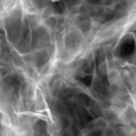
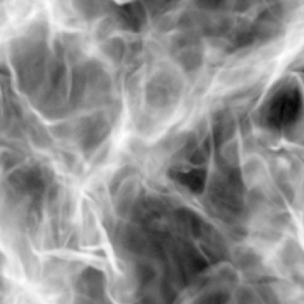
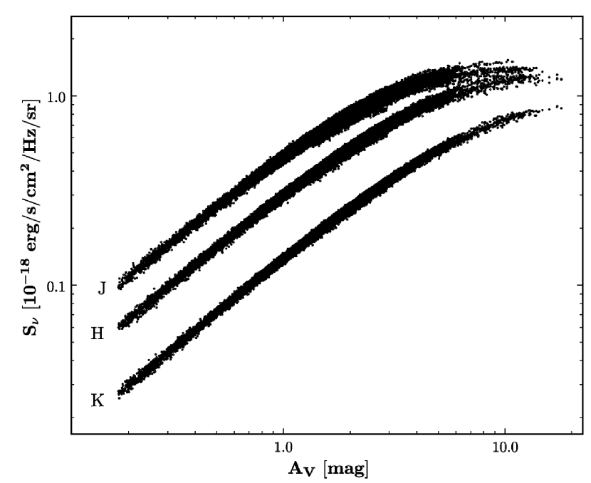
The left panel of Figure 1 shows a projection of the density field from the turbulence simulation described above. The corresponding image of scattered light in the H band is shown on the right panel of the same figure, for the model with mean gas density cm-3. The H band scattering reproduces well the spatial structure of the cloud model. The same is true for the J and K bands as well (not shown for lack of space). The scattered light tends to saturate only in the densest regions, at approximately 5, 10 and 20 magnitudes of visual extinction for the J, H and K bands respectively, as illustrated in the left panel of Figure 2.
Based on the radiative transfer along a single line of sight we may assume that the observed intensity can be approximated with the function
| (1) |
where is the column density. The coefficients and are positive constants defined for each band. They are related to dust properties and to the strength of the radiation field illuminating the cloud. To first order in (small column densities), Eq. 1 gives
| (2) |
so the intensity is proportional to the column density. At large values of column density the relation is not linear, but can still be derived by comparing different bands. For example, by writing Eq. 1 for the H and K bands, can be eliminated and the H band can be expressed as a function of the K band,
| (3) |
The coefficients , , and and the ratios and can be determined by fitting this curve to the observations (this is actually done in the three–dimensional (J,H,K) space).
The coefficients depend mainly on the properties of the dust grains. They should be well defined, since dust properties are believed to be very constant in the NIR. Their absolute values can be obtained from previous observations of similar objects or by using stellar extinction measurements to fix the scale in the current observations. The coefficients depend on the radiation field that illuminates the cloud. However, the spectrum of the incoming radiation can be directly estimated using observations at low extinction, and the field strength appears basically as a multiplicative factor in the estimated column densities.
The same deep observations carried out to detect the NIR scattering also provide color excesses for a large number of background stars. The intensity of the incoming radiation can be determined by comparing the stellar extinction with the amount of scattered light. All the coefficients can also be obtained from radiative transfer models based on the assumed dust properties and radiation field strength. Once the coefficients are determined, Eq. 1 defines, as a function of column density, a fixed curve in the three-dimensional (J,H,K) space. Column densities are estimated by finding the closest point on this curve to each observed (J,H,K) triplet and solving for in Eq. 1.
We have applied this method to the numerical cloud model described above. Noise is first generated so the signal–to–noise ratios for the mean intensities in the J, H,and K bands are 15, 10 and 7, respectively. The radiative transfer model gives = 1.04, 0.83, 0.54 and = 0.019, 0.012, 0.0074 , based on the true column densities and the scattered light observed toward one direction of the cloud model. With these coefficients, the column density for a different, orthogonal viewing direction is then estimated using the ’observed’ surface brightness in that direction.
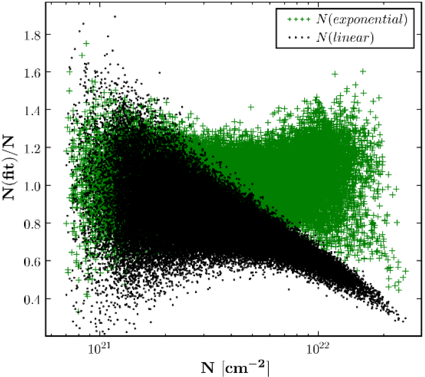
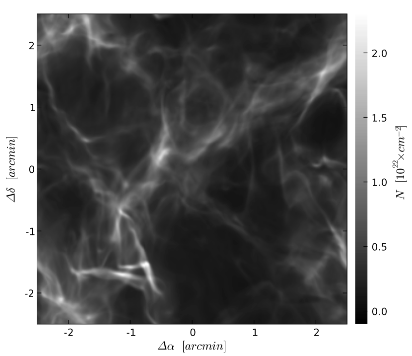
Figure 3 shows the ratio between the estimated column densities and the true column density. The uncorrected values obtained assuming a linear relation between the H–band intensity and the column density are also shown. In regions with mag the correction is almost a factor of three, or a factor 2 if compared with uncorrected K–band intensities. Without correction, the estimated column densities are on the average approximately 25% below the correct value. Fig. 3 shows that the corrected estimates remain unbiased even at large extinctions, mag. Their mean value deviates only 0.2% from the correct one, and the scatter around the mean is 10%.
In Fig. 2a the scatter is real (no noise was added there) and due mostly to spatial variations in the field strength within the cloud. The field becomes more attenuated toward the cloud center, reducing the ratio of surface brightness to column density. In other words, the coefficients in Eq. 1 are functions of position. This is the dominant source of the scatter in Fig. 3 as well. Model calculations may be used to estimate the large scale variations in the field strength, and to remove most of this scatter. A detailed radiative transfer calculation could also be carried out, where the cloud model is iteratively built to replicate the observations as close as possible. The estimated column densities would then only be subject to uncertainties in the cloud structure along the line of sight. Other effects could be modeled as well, for example a non–isotropic radiation field.
5. Conclusions
The average surface brightness of scattered light in the model with mean gas density cm-3 was , and erg cm-2 Hz-1 sr-1 in the J, H and K bands respectively. For a target signal–to–noise of 15, 10, and 7 for the J, H, and K bands respectively, the necessary integration times for the SOFI instrument on the 3.6 m NTT telescope become 33, 80, and 250 hours. However, the instrument has 0.29 pixel size, and if resolution is degraded to 0.6 the quoted signal–to–noise ratios can be reached with less than 100 hours of integration. With ISAAC/VLT, the same noise level per 0.15 pixel requires 22+72+196=290 hours. For a resolution decreased to 0.6, the integration time is reduced to 17 hours.
At a distance of 300 pc, the angular resolution of 0.1 that can be achieved with adaptive optics, corresponds to a spatial resolution of AU. Imaging of near–IR scattering is therefore capable of probing the structure of nearby interstellar clouds at unprecedented spatial resolution, down to a physical scale of the order of the size of circumstellar disks, the gyroradius of GeV cosmic rays or the Kolmogorov turbulence dissipation scale.
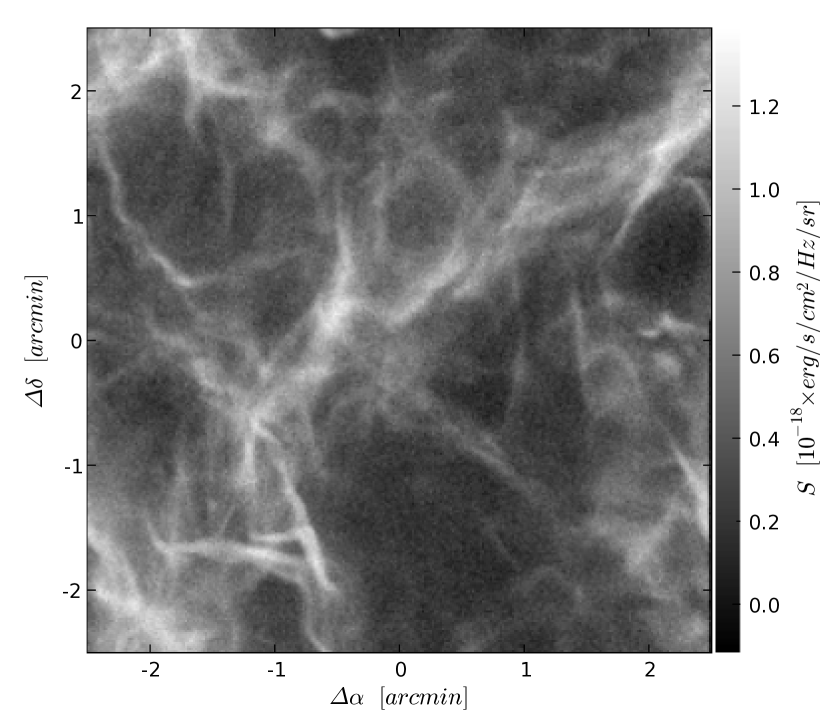
The right panel of Figure 2 shows the H band of our model. The image is composed of pixels. After decreasing the resolution to 0.6, the same noise level and angular dynamical range is reached with ISAAC/VLT in 17 hours. This example shows that imaging of near–IR scattering is a promising method also for relatively large scale surveys of interstellar clouds, especially with the new generation of wide–field instruments, such as WFCAM on UKIRT and WIRCam on CFHT. As discussed in the previous section, the method can provide a rather accurate estimate of the column density, preferentially at values of visual extinction between approximately 1 and 20 magnitudes, and even below one magnitude if complemented with shorter wavelengths. It is therefore ideal for the study of low and medium density interstellar clouds, and less suitable for the interior of very dense protostellar cores.
References
- Draine (2003) Draine B. 2003, ApJ 598, 1017
- Foster & Goodman (2005) Foster, J. & Goodman, A. 2005, in preparation
- Juvela (2005) Juvela M. 2005, A&A, 440, 531
- Juvela & Padoan (2003) Juvela M., Padoan P. 2003, A&A 397, 201
- Mathis, Mezger & Panagia (1983) Mathis J.S., Mezger P.G., Panagia N. 1983, A&A, 128, 212
- Padoan & Nordlund (1999) Padoan, P., & Nordlund, Å. 1999, ApJ, 526, 279
- Padoan et al. (1999) Padoan, P., Bally, J., Billawala, Y., Juvela, M., & Nordlund, Å. 1999, ApJ, 525, 318
- Padoan et al. (2001) Padoan, P., Juvela, M., Goodman, A. A., & Nordlund, Å. 2001, ApJ, 553, 227
- Padoan et al. (2004) Padoan, P., Jimenez, R., Juvela, M., & Nordlund, Å. 2004, ApJ, 604, L49
- Yusef et al. (1994) Yusef-Zadeh F., Morris M., White R.L. 1984, ApJ 278, 186