The Deuterium, Oxygen, and Nitrogen Abundance Toward LSE 44

Abstract

We present measurements of the column densities of interstellar D I, O I, N I, and H₂ made with the Far Ultraviolet Spectroscopic Explorer (FUSE), and of H I made with the International Ultraviolet Explorer (IUE) toward the sdO star LSE 44 [($l$,$b$) = (313$\fdg$37, +13$\fdg$49); d = $554\pm 66$ pc; z = $+129\pm 15$ pc]. This target is among the seven most distant Galactic sight lines for which these abundance ratios have been measured. The H I column density was estimated by fitting the damping wings of interstellar Ly$\alpha$. The column densities of the remaining species were determined with profile fitting analyses, and supplemented with curve of growth analyses for O I and H₂. We find log $N$(D I) = $15.87\pm 0.08$, log $N$(O I) = $17.57^{+0.21}_{-0.15}$, log $N$(N I) = $16.43\pm 0.14$, and log $N$(H I) = $20.52^{+0.20}_{-0.36}$ (all errors $2\,\sigma$). This implies D/H = $(2.24^{+1.39}_{-1.32})\times 10^{-5}$, D/O = $(1.99^{+1.30}_{-0.67})\times 10^{-2}$, D/N = $(2.75^{+1.19}_{-0.89})\times 10^{-1}$, and O/H = $(1.13^{+0.96}_{-0.71})\times 10^{-3}$. Of the most distant Galactic sight lines for which the deuterium abundance has been measured LSE 44 is one of the few with D/H higher than the Local Bubble value, but D/O toward all these targets is below the Local Bubble value and more uniform than the D/H distribution.

1. Introduction

Precise measurements of primordial abundances of the light elements deuterium (D), ³He, ⁴He, and ⁷Li relative to hydrogen have been a goal of astronomers for many years. In the standard Big Bang nucleosynthesis model, these quantities are related in a straightforward way to the baryon-to-photon ratio in the early universe, from which $\Omega_{\rm B}$, the fraction of the critical density contributed by baryons, may be determined (Boesgard & Steigman 1985). Since deuterium is easily destroyed in stellar interiors (astration), and no significant production mechanisms have been identified (Reeves et al. 1973; Epstein, Lattimer, & Schramm 1976), the D/H ratio is expected to monotonically decrease with time.

Precise measurements of D/H in the local interstellar medium (ISM) were first made using Copernicus (Rogerson & York 1973), HST (Linsky et al. 1995), and IMAPS (Jenkins et al. 1999; Sonneborn et al. 2000). In the last several years many additional measurements of D/H, D/O, D/N, and related species, have been made using FUSE (Moos et al. 2002; Hébrard & Moos 2003; Wood et al. 2004). These local ISM measurements represent a lower limit to the primordial value. When corrected for the effects of astration (Tosi et al. 1998), the results should be comparable to those obtained in low-metallicity, high redshift Ly$\alpha$ clouds (Crighton et al. 2004; Kirkman et al. 2003), which should be very nearly the primordial value itself.

As data on more sight lines has accumulated the situation is not as simple as originally envisioned. At high redshift, measurements of D/H vary from $(1.6-4)\times 10^{-5}$ (Crighton et al. 2004; Pettini & Bowen 2001), despite the fact that the metallicity in all these environments is low enough to suggest that D/H should match the primordial value. More locally, it is now accepted that for sight lines within the Local Bubble, a region of hot, low-density gas (Sfeir et al. 1999) within a distance of $100-150$ pc and log $N({\rm H\;\mbox{\small\rm I}})$$\lesssim 19.2,$ in which the Sun lies, D/H is nearly constant, but the value is uncertain. Based on measurements toward 16 targets, Wood et al. (2004) state that (D/H)${}_{LB}=1.56\pm{0.04}\times 10^{-5}$. Alternatively, (D/H)_LB may be inferred from measurements of D/O and O/H. Hébrard & Moos (2003) discuss the advantages of this approach, including potential reduction of systematic errors associated with measuring $N({\rm D\;\mbox{\small\rm I}})$and $N({\rm H\;\mbox{\small\rm I}})$ directly, which differ by five orders of magnitude. Their approach relies on the observed high spatial uniformity of O/H (Meyer, Jura, & Cardelli 1998; Meyer 2001; André et al. 2003). The result is (D/H)${}_{LB}=1.32\pm{0.08}\times 10^{-5}$, about $2\sigma$ different than the Wood et al. value.

At distances greater than $\sim 500$ pc, or more precisely, at log $N({\rm H\;\mbox{\small\rm I}})$$\gtrsim 20.5,$ the few sight lines measured have lower D/H. Based on a suggestion originally made by Jura (1982) and extended by Draine (2004a, 2004b) that under the right thermodynamic conditions deuterium can be depleted onto dust grains, Wood et al. (2004) have interpreted D/H variations as being due to various levels of depletion and, over the longer sight lines, the effects of averaging the D/H concentration over multiple clouds along the sight line. In this scenario, the low value at large distances represents the gas phase abundance in the local disk, (D/H)${}_{LDg}=(0.85\pm 0.09)\times 10^{-5},$ and one must include the depleted deuterium to determine the total deuterium abundance. An alternate explanation is offered by Hébrard & Moos (2003). Based on D/O, D/N, and D/H measurements, they suggest that the low gas-phase value observed at high column densities and distances is the true Galactic disk value, and there is not a significant reservoir of deuterium trapped in dust grains. D/H has an unusually high value in the Local Bubble if this interpretation is correct. The reason for this high value is not understood. One possibility is the infall of primordial, deuterium-rich material, and another is non-primordial deuterium production, such as in stellar flares. This is discussed further in §5.

To test this hypothesis it is necessary to make additional measurements of D I, H I, O I, N I, H₂, and additional species that might yield information about depletion and physical conditions, toward targets with log $N({\rm H\;\mbox{\small\rm I}})$$\gtrsim 20.5$ In this paper we present the results of an analysis of the sight line toward LSE 44, an sdO star located at a distance of $554\pm 66$ pc and well within this column density regime. We derive D I, O I, N I, and H₂ column densities with data obtained from the Far Ultraviolet Spectroscopic Explorer (FUSE) and estimate the H I column density with data from the International Ultraviolet Explorer (IUE).

In §2 we present a summary of the observations and a description of the data reduction processes. In §3 the stellar properties of LSE 44 are discussed. The details of the analysis of the D I, O I, N I, and H₂ column densities are given in §4, and the H I analysis is presented in §5. In §6 we discuss the results of this study.

2. Observations and Data Processing

The FUSE instrument consists of four co-aligned spectrograph channels designated LiF1, LiF2, SiC1, and SiC2, named for the coatings on their optics, which were selected to optimize throughput. Each channel illuminates a pair of microchannel plate segments, labeled A and B. The LiF channels have a bandpass of approximately 1000-1187 Å  and the SiC channels approximately 910-1090  Å. Thus, each observed spectral line may appear in the spectra from multiple channels. The FUSE resolution is approximately 20 km s^-1 (FWHM), but it varies slightly between channels, and within a channel, as a function of wavelength. A detailed description of the FUSE instrumentation and performance is given by Sahnow et al. (2000).

LSE 44 was observed with FUSE for a total of 86 ksec under programs P2051602 - P2051609. A total of 119 exposures are in the MAST archive, obtained with various levels of alignment success for the separate channels, and some were obtained when one or both detectors were not at full voltage. The observation log is shown in Table 1, and the total exposure time by channel is shown in Table 2. All data were obtained in time-tag mode with focal-plane offsets (FP-SPLITS) in the MDRS ($20\arcsec\times 4\arcsec$) aperture.

The data were reduced using CALFUSE pipeline version 3.0.6. We used the default pixel size of 0.013Å. The signal-to-noise ratio per pixel in the continuum region around 928Å for both SiC1B and SiC2A spectra is typically about 3.5 in individual, well-aligned exposures of $\sim 900$s, the maximum duration of any exposure. The individual 1-dimensional spectra were co-added to form the final spectrum for each channel and detector segment separately after removing the relative shifts between individual spectra on the detector caused by image and grating motion (Sahnow et al. 2000). The shifts were determined by cross-correlating the individual spectra over a limited wavelength range which contained prominent spectral features but no airglow lines. Typical shifts were $\lesssim 4$ pixels, or $\lesssim 0.050$Å. The S/N ratios in the summed spectra are approximately 26 and 27, respectively, for the SiC1B and SiC2A channels. Narrow interstellar absorption features in the summed spectra do not exhibit unexpected broadening, indicating that the summing process did not smear the data. Although FUSE observations of H I and O I lines are sometimes contaminated by airglow emission, data obtained during spacecraft orbital night showed that this was unimportant in our analysis, so the combined day and night data were used.

Figure 1 shows the co-added SiC1B spectrum of LSE 44, which covers the wavelength range $915\sim 990$Å. D I, O I, N I, and H₂ lines arising in the ISM are identified.

The H I column density along this line of sight was estimated using the Ly$\alpha$ profile from the single high resolution spectrum of LSE 44 taken with IUE. The 16.5 ksec observation was made on 29 August 1986 (see Table 1), and reduced using IUESIPS. The analysis of this data is discussed in more detail in §4.4.

3. Stellar Properties of LSE 44

In his survey of subluminous O stars, Drilling (1983) obtained photometric and spectroscopic data for LSE 44. His $UBV$ photometry gives $V=12.45$, $B-V=-0.24$, and $U-B=-1.18$ (Table 3), and indicates that the star is relatively hot. He describes the optical spectrum of LSE 44 by saying that the only lines present are the He II $\lambda$4686 line and the Balmer series. He adds that the appearance of these lines is very similar to those in the spectrum of the sdOB star Feige 110, but the Balmer lines are stronger and the He II $\lambda$4686 line is weaker in the spectrum of LSE 44 (see, e.g., Heber 1984; Friedman et al. 2002). In order to measure the atmospheric parameters of LSE 44, D. Kilkenny (2004, private communication) obtained an optical spectrum of LSE 44 at the South African Astronomical Observatory with the 1.9-m telescope and CCD spectrograph. The optical spectrum covers the wavelength range 3400 – 5400 Å with a resolution of about $\sim 3$ Å. The normalized spectrum is plotted in Figure 2. As reported by Drilling (1983), our optical spectrum shows broad Balmer lines starting from H$\beta$ to H$\theta$ and the He II $\lambda$4686 line, which is the only helium line detected in this spectrum. The Ca II K $\lambda$3935 line is also detected in the optical spectrum.

The atmospheric parameters of LSE 44 were obtained by fitting the optical spectrum illustrated in Figure 2 with a grid of synthetic spectra and by using the Marquardt method (see, Bevington & Robinson 1992). This method optimizes the effective temperature, gravity, and helium abundance in order to obtain a model that best matches the observed spectrum. We computed a grid of NLTE H/He atmosphere models with 20,000 K $\leq T_{\rm{eff}}\leq 80$,000 K in steps of 2,000 K, for different values of the surface gravity $4.8\leq\log g\leq 6.4$ in steps of 0.2 dex, and for different helium abundances $-4.0\leq\log N({\rm{He}})/N({\rm{H}})\leq 0.0$ in steps of 0.5 dex. The models were computed with the stellar atmosphere codes TLUSTY and SYNSPEC (see, e.g., Hubeny & Lanz 1995). Figure 2 shows our best fit for the optical spectrum of LSE 44. We obtain $T_{\rm{eff}}=38$,700$\pm 1$,000 K, $\log g=5.5\pm 0.1$, and $\log N({\rm{He}})/N({\rm{H}})=-2.8\pm 0.1$. We used these atmospheric parameters to compute the stellar Ly$\alpha$ line profile in order to measure the H I column density toward LSE 44. (see §4.4).

The evolutionary status and physical properties of LSE 44 can be estimated by comparing its position in a $T_{\rm{eff}}$-$g$ diagram with evolutionary sequences. Figure 3 shows the position of LSE 44 in such a diagram with the positions of a sample of hot subdwarf B stars (sdB). It also shows post-extreme horizontal branch (post-EHB) evolutionary sequences that were computed by B. Dorman (1999, private communication). The position of LSE 44 in the $T_{\rm{eff}}$-$g$ diagram suggests that it is an sdB star that has evolved from the EHB. Even though LSE 44 is classified as an sdO star based on its optical spectrum, it relates to the sdB stars. sdB stars have effective temperatures and gravities in the ranges 24,000 K $\lesssim T_{\rm{eff}}\lesssim 40$,000 K and $5.0\lesssim\log g\lesssim 6.2$, and helium abundances that are typically a factor of ten smaller than solar (see, e.g., Saffer et al. 1994). The evolutionary sequences in Figure 3 represent the evolution of typical sdB stars that have helium-burning cores of $\sim 0.477$ M_⊙ and small hydrogen envelopes $M_{\rm{env}}\lesssim 0.0045$ M_⊙. Each evolutionary track corresponds to models with about the same helium core mass but with different hydrogen envelope masses. In these models the hydrogen envelopes are too small to ignite the hydrogen burning shell, and therefore the stars appear subluminous, hot, and compact. In Figure 3 the hatched region corresponds to the zero-age EHB (ZAEHB). In this way, an EHB star evolves from the ZAEHB and moves first to the right and then to the left toward the white dwarf region without reaching the asymptotic giant branch (AGB). A star spends $\sim 10^{8}$ yr on the EHB and $\sim 10^{7}$ yr off the EHB en route to the white dwarf region.

The spectral type sdO is a spectroscopic class that includes stars showing strong Balmer lines and He II lines. Because of its high effective temperature and low helium abundance, LSE 44 appears as an sdO star. The evolutionary tracks surrounding the position of LSE 44 show that stars in this portion of the $T_{\rm{eff}}$-$g$ diagram have left the helium core burning phase and undergo a helium shell burning phase. One can assume that the mass of LSE 44 is $\sim 0.4775$ M_⊙ and estimate its distance by using the expression

$$D=\sqrt{\frac{GM}{g}\frac{4\pi\,H_{V}}{F_{0,V}}}\;10^{0.2(V-A_{V})},$$ (1)

where $G$ is the gravitational constant, $M$ is the mass of the star, $g$ is the gravitational acceleration, $H_{\nu}$ is the Eddington flux weighted by the Johnson passband $V$ of Bessel (1990), $F_{0,V}$ is the average absolute flux of Vega at $V$ as specified in Heber et al. (1984), $V$ is the apparent visual magnitude, and $A_{V}$ is the interstellar absorption. By using the best model fit parameters and the passbands of Bessel (1990) we computed the intrinsic color index $(B-V)_{0}$ and obtained the color excess $E(B-V)=0.05\pm 0.03$, which gives $A_{V}=0.155\pm 0.093$ when using $R_{V}=3.1$. The distance to LSE 44 is then $554\pm 66$ pc.

The FUSE spectrum of LSE 44 shows many photospheric and interstellar absorption lines. The strongest photospheric lines are the Lyman series that start at Ly$\beta$ and go up to lines close to the series limit. Because of the high gravity the photospheric Lyman lines merge together before reaching the series limit, and the remaining Lyman lines close to this limit are mainly due to interstellar H I. The other strong photospheric lines are He II $\lambda$1084, C III $\lambda\lambda$1175, N III $\lambda\lambda$1184, N IV $\lambda\lambda$923 and $\lambda$955, Si IV $\lambda\lambda$1126 and $\lambda$1066, P V $\lambda\lambda$1123, S IV $\lambda\lambda$1070, and S VI $\lambda\lambda$937. There are also many fainter unidentified stellar lines that depress the continuum. For instance, Figure 4 shows a comparison between the FUSE spectra of LSE 44 and the sdOB star Feige 110 ($T_{\rm{eff}}=42$,300 K and $\log g=5.95$; Friedman et al. 2002). The figure illustrates that both stars have many lines in common, but because of the lack of atomic data, we cannot identify these absorption lines. The Si IV lines at 1122.49 Å and 1128.33 Å and the P V line at 1128.008 Å are practically the only stellar lines that can be identified in these portions of the FUSE spectrum. This example illustrates clearly that blends of unidentified stellar lines with interstellar lines could lead to systematic errors when measuring interstellar column densities.

Table 3 summarizes the important properties of LSE 44 and the sight line to this star.

4. Interstellar Column Density Analyses

Two techniques have been used to estimate the column densities in this analysis. The first involves directly measuring the equivalent widths of absorption lines, which are fit to a single-component Gaussian curve-of-growth (COG) (Spitzer 1978). Although it appears from the line widths that the line of sight may traverse more than a single velocity component, no high resolution optical or UV spectrum exists which would allow us to model a more complicated velocity structure. We therefore made the simplifying assumption that a single interstellar cloud with a Maxwellian velocity distribution is responsible for the absorption. The estimates of the column density ($N$) and Doppler parameter ($b$) derived from the COG are likely to include systematic errors due to this assumption. For example, the derived $b-$value will not be a simple quadrature combination of thermal and turbulent velocity components, as it would be for a true single cloud. Instead, it will also reflect the spread in velocities of the multiple clouds that are likely to lie along a sight line of this length. Jenkins (1986) has discussed the systematic errors associated with the COG technique when there are multiple clouds of various strengths along a sight line, and has shown that if many non-saturated lines are used, and if the distribution of $N$ and $b-$values in the clouds is not strongly bimodal, then the column density is likely to be underestimated by $\lesssim$ 15%.

Despite these shortcomings, the COG technique has the virtue of being unaffected in principle by convolution with the instrumental line spread function (LSF). In practice, it must be used with caution because of the problem of blending with neighboring lines and, especially for a target like LSE 44, because it is difficult to establish the proper continuum in some spectral regions, presumably due to the presence of many unidentified stellar absorption features.

The second technique is profile fitting (PF). For all species except H I we used the code Owens.f, which has been applied to FUSE spectra for many previous investigations. This code models the observed absorption lines with Voigt profiles using a $\chi^{2}$ minimization procedure with many free parameters, including the line spread function, flux zero point, gas temperature, and turbulent velocity within the cloud. We split each spectrum into a series of small sub-spectra centered on absorption lines, and fit them all simultaneously. Each fit typically includes about 60 spectral windows, and approximately 100 transitions of H I, D I, O I, N I, and H₂ ($J=0$ to $5$). The wavelengths and oscillator strengths of the lines used in the profile fitting analysis are given in Table 4. Note that there are fewer than 100 entries in the table because some lines appear in multiple detector segments. D I, O I, and N I were assumed to be in one component, H₂ in a second, and H I in a third. Velocities between windows were allowed to shift to accommodate inaccuracies in the FUSE wavelength calibration. The line spread function (LSF) is fixed within a spectral window, but is allowed to change in a given detector segment from one window to another, and between segments. This is consistent with the performance of the FUSE spectrographs (Sahnow et al. 2000). No systematic relationship between the LSF and the derived column density or $b-$value of any species was observed.

Only one interstellar component for a given species was assumed along the sight line although this is unlikely to be true for such a distant target. Hébrard et al. (2002) discuss tests they performed on an extensive list of potential systematic errors using profile fitting, including the single component assumption. In these tests they found that fits obtained with up to five interstellar components gave the same total column density within the 1 $\sigma$ error bars, as long as saturated lines are excluded from the analysis, which we have been careful to do. Thus, we report total integrated column densities along the sight line.

It is possible that the temperature and turbulent velocities differ from one cloud to another. To test this we did profile fits with D I, O I, and N I in three independent components. The column density estimates differ by less than 1 $\sigma$ from those obtained by assuming a single component. The $b-$values also agree with that obtained by assuming a single component, although they are not well-constrained because only unsaturated lines are used. These species could also have different ionization states if they reside in clouds with different temperatures. However, the ionization potentials of D I and O I and, to a slightly lesser extent, N I  are so similar that this is unlikely to be a problem.

The Fe II absorption lines detected in the spectrum are abnormally broad for interstellar lines, about 10 km s^-1, with a temperature of $\sim 2\times 10^{5}$ K, compared to $\sim 6$ km s^-1 for N I and O I (see §4.2). The cause of this broadening is not known, but Fe II is not present in the stellar atmosphere because the temperature is too high. In the fits we did not include Fe II in the component containing D I, O I, and N I, but this has no effect on the determination of the interstellar column densities of these species.

All laboratory wavelengths and oscillator strengths used in this work are from Morton (2003) and Abgrall et al. (1993a, 1993b). Neither the COG nor profile fitting techniques include oscillator strength uncertainties in the error estimates. The application of Owens.f to FUSE data is described in greater detail by Hébrard et al. (2002).

4.1. The D I Analysis

We determined $N({\rm D\;\mbox{\small\rm I}})$ using only the profile fitting technique. We attempted to construct a COG, but we were unable to determine unambiguously the proper placement of the continuum in the presence of the strong H I lines separated from the D I lines by +81 km s^-1. The situation is particularly difficult for this sight line due to the unusual shape of the neighboring continuum around the $\lambda 916.180$ line, and the unaccounted for absorption on the red wing of the H I $\lambda 920.712$ line. Our tests indicated that failure to recognize such problems caused COG estimates of $N({\rm D\;\mbox{\small\rm I}})$ to be approximately 0.3 dex too low. Once the continuum is defined in the COG analysis, it is fixed. By contrast, although continuum placement errors will also lead to column density errors with profile fitting, this technique allows the shape of the continuum to change as part of the fitting process. The continuum was modeled with polynomials of order $0-4$ to allow for a large range of continuum fits. We required acceptable fits simultaneously to all five D I lines used in the analysis (see below). In addition, removing any of the lines from the analysis did not change the final column density estimate significantly. This was not true for the COG fit, which was highly sensitive to the continuum placement at the $\lambda 916.180$ line. Removal of this line changed the COG result by more than 0.2 dex. Therefore, by virtue of its simultaneous and self-consistent fit over multiple lines, and its sensitivity to the exact way in which D I blends with the blue wing of the neighboring H I line, profile fitting is the best method for measuring the deuterium column density.

Five D I absorption profiles over three separate spectral lines were used in the profile fits: $\lambda 916.180$ in the SiC1B channel, and $\lambda 919.100$ and $\lambda 920.712$ in both the SiC1B and SiC2A channels. Longer wavelength D I lines are too saturated to provide additional constraints on the column density estimate, and the convergence of the H I Lyman series precludes using shorter wavelength lines. The D I $\lambda 916.931$ and $\lambda 917.880$ lines are too strongly blended with O I and H₂ lines to be used. Although the same transition observed in separate FUSE channels potentially are subject to systematic errors arising from similar effects, such as continuum placement and blending, they do represent independent measurements with distinct spectrographs. Thus, we include all five profiles in our analysis.

To properly measure the interstellar D I, the effects of the stellar H I Lyman series and He II absorption must be removed. This was done in two ways. First, the stellar model described in §3 was shifted in velocity space and scaled in flux until the stellar H I damping wings matched the observed spectrum away from the cores of the interstellar H I lines. The resulting average velocity difference was $\Delta V\equiv V_{*}-V_{\rm ISM}=-39\pm 5$ km s^-1 and $-32\pm 13$ km s^-1 for the SiC1B and SiC2A spectra, respectively. This compares favorably to $\Delta V=-33\pm 6$ km s^-1 based on the measured velocities in the high-dispersion IUE spectrum of photospheric lines (N IV, N V, O VI, Si VI, S V, C III, and C IV) and interstellar lines (Si II, Si III, and S II). The spectral resolution of IUE in this mode is approximately 25 km s^-1 (FWHM).

The stellar model is only an approximation of the true absorption from the atmosphere of LSE 44. Since not all species present in the atmosphere are properly accounted for in the model, and since some of the atomic constants included in the model are not well-known, using the model may in fact introduce systematic errors. To check for this we also applied the profile fitting without the model, using instead up to a fourth-order polynomial to fit the stellar spectrum and continuum. This method has been used many times before in similar analyses; see, for example, Hébrard & Moos (2003). As described below, the two methods give column densities which agree within the errors.

Several parameters are free to vary through the fits, including the column densities, the radial velocities of the interstellar clouds, and the shapes of the stellar continua. Some instrumental parameters are also free to vary, including the widths of the Gaussian line spread function (LSF), which is convolved with the Voigt profiles within each spectral window. The averaged width of the LSF that we found is 5.8 pixels, with a 0.8-pixel $1\,\sigma$ dispersion (full widths at half maximum). These FUSE pixels are associated with CALFUSE version 3, and are 0.013Å in size. Note that CALFUSE versions 1 and 2, which was used in most previously published FUSE studies, produced pixels approximately half this size. This explains why the LSF reported previously was approximately about 11 pixels wide (see, e.g., Friedman et al. 2002; Hébrard et al. 2002). Some examples of fits are plotted in Figure 5.

Using the stellar model we find log $N$(D I)${}_{sm}=15.84\pm{0.08}$. Using a polynomial fit to the stellar plus interstellar continuum, we find $N$(D I)${}_{poly}=15.89\pm{0.08}$. These errors include our estimates of the systematic errors associated with the stellar normalization. Our final estimate is the mean of these two values, log $N({\rm D\;\mbox{\small\rm I}})$= $15.87\pm{0.08},$ where the error of the mean has not been reduced below the individual values since $N$(D I)_sm and $N$(D I)_poly are not independent estimates of the column density.

4.2. The O I Analysis

The continuum placement problem is much less severe for the O I lines because the spectral regions adjacent to the lines used in the analysis are generally smooth and well-behaved, without the presence of very strong adjacent lines. Thus, we use both the profile fitting and curve-of-growth techniques to estimate $N({\rm O\;\mbox{\small\rm I}})$. The profile fitting analysis used only the O I $\lambda 974.070$ line, because this line is almost completely unsaturated. We did verify that the fit to other O I lines in the spectrum was acceptable, but they provide almost no additional constraint on the column density because they are saturated. One might be concerned that an erroneous $f-$value for this transition would cause an inaccurate estimate of $N({\rm O\;\mbox{\small\rm I}})$. However, Hébrard et al. (2005) discuss this issue, and show that it is consistent with column densities derived from stronger O I lines in the case of BD+28$\arcdeg 4211,$ and derived from the weak $\lambda 1356$ intersystem line in the case of HD 195965. The O I $\lambda 974.070$ line is blended with two H₂ lines, Lyman 11-0R(2) $\lambda 974.156$ and Werner 2-0Q(5) $\lambda 974.287,$ and absorption from these species was accounted for when calculating $N({\rm O\;\mbox{\small\rm I}})$, as described below. There is also an H₂ $J=6$ line at nearly the same wavelength, but the column density in this rotational level is too small to be of concern. The result of our analysis is $N$(O I)${}_{pf}=17.53^{+0.25}_{-0.15}.$

To construct the curve-of-growth the equivalent widths of the O I lines were measured in the following way. First, low-order Legendre polynomials were fitted to the local continua around each O I line. The lines were integrated over velocity limits chosen to exclude absorption from adjacent lines. Only isolated lines were selected so that no deblending was required. Scattered light remaining after the CALFUSE 3 reduction is negligibly small, and no additional correction was required. The measured equivalent widths are given in Table 5. The estimated errors from this method are described in detail by Sembach & Savage (1992). They include contributions from both statistical and fixed-pattern noise in the local continuum. Continuum placement is particularly difficult and subject to error due to the presense of many unidentified stellar lines. To estimate the magnitude of such errors, we did trials in which we drew the continuum at its maximum and minimum plausible locations, and compared the calculated equivalent widths with the best estimated placement. We added 2 mÅ to the error of each measured O I line equivalent width to account for these placement errors. This is consistent with the magnitude of this systematic error determined in previous analyses of similar sight lines (e.g., Friedman et al., 2002).

Due to the blending with the H₂ lines we initially did not include the O I $\lambda 974.070$ line. However, this line is extremely important because it is the only O I line that is not substantially saturated, and therefore provides the greatest constraint on $N({\rm O\;\mbox{\small\rm I}})$. We constructed curves of growth for the $J=2$ and $J=5$ rotational levels of H₂, calculated column densities and $b-$values, determined the appropriate Voigt profiles, and used them to remove the H₂ signature from the blended line. Then the equivalent width of the O I line was measured in the usual way. The H₂ analysis is described in Section 4.5. The O I curve of growth is shown as the solid line in Figure 6. The best fit column density is log $N$(O I)${}_{COG}=17.59^{+0.13}_{-0.14}$. Combining this with our profile fitting result, we arrive at our best estimate of the O I column density, log $N({\rm O\;\mbox{\small\rm I}})$= $17.57^{+0.21}_{-0.15}.$

We note that the O I $\lambda 919.917$ line has been excluded from the analysis. We were unable to get a good fit of this line with profile fitting, and it fell well below the curve-of-growth. This is also true for Feige 110 (Hébrard et al. 2005), whose spectrum is similar in many respects to that of LSE 44, as discussed in §3. It is unlikely that this line has a significantly incorrect $f-$value since the absorption from this line is consistent with absorption from other O I lines in, for example, the spectrum of BD+$28\arcdeg 4211$ (Hébrard & Moos 2003). It is possible that there is unidentified absorption adjacent to this line, which depresses the local continuum, causing an underestimate of the equivalent width of this line. Alternatively, the location of this line on the COG may be an indication that there are multiple components along the sight line, with different column densities. This would cause a ”kink” in the COG, which might be more obvious if additional O I lines were available to include on the plot. However, with no high resolution spectra available, we are unable to confirm this hypothesis. If we include the $\lambda 919.917$ line, the single-component COG gives log $N({\rm O\;\mbox{\small\rm I}})$= $17.52^{+0.22}_{-0.23}$ and $b=6.33^{+0.49}_{-0.44},$ which is shown as the dashed line in Figure 6. This differs from our best estimate column density by less than $1\sigma.$

It is worth emphasizing the importance of non-saturated lines in the determination of $N({\rm O\;\mbox{\small\rm I}})$  even at the expense of the potential introduction of systematic errors associated with using strongly blended lines. Computing a COG excluding the O I $\lambda 974.070$ (and $\lambda 919.917$) lines gives $N$(O I) = $17.22^{+0.55}_{-0.29}$, about $2\sigma$ less than the result obtained when including the weak line. This is shown as the dotted line in Figure 6. The fit to the remaining spectral lines is quite acceptable, but is clearly inconsistent with the weak line. Indeed, this line was not used in the initial analysis of Feige 110 (Friedman et al. 2002). We have recently included $\lambda 974.070$ in a re-analysis of $N({\rm O\;\mbox{\small\rm I}})$ along this sight line. The COG and profile fitting methods are now in good agreement, and the column density estimate has increased by 0.33 dex compared to the original estimate. This is discussed more fully in Hébrard et al. (2005).

4.3. The N I Analysis

As was the case with D I, only profile fitting was used to determine $N({\rm N\;\mbox{\small\rm I}})$. The COG technique was not used because of the uncertainties in establishing continuum levels on each side of the N I lines.

Three lines were used in the profile fitting analysis: $\lambda 951.079,\lambda 951.295,$ and $\lambda 955.882$. The method is the same as was used for the deuterium analysis, and is described in §4.1. The result is log $N$(N I) = $16.43\pm 0.14.$

4.4. The H I Analysis

In the direction of LSE 44, the Ly$\alpha$ line provides the best constraint on the total H I column density because its radiation damping wings are very strong. However, Ly$\alpha$ is not accessible to FUSE. Ly$\beta$ displays modest damping wings, and we attempted to model the absorption profile in order to estimate $N({\rm H\;\mbox{\small\rm I}})$. We were unable to do this primarily because of the presense of two H₂ lines, J=0 $\lambda 1024.230$ and J=2 $\lambda 1026.526$, on the blue and red wings of the Ly$\beta$ absorption, respectively. As discussed in §4.5, all lines of H₂ in the J=0 rotational level lie on the flat portion of the COG, so we are unable to make even a rough estimate of the column density. The situation for J=2 is only slightly better, with the weakest lines still considerably saturated. Since these lines are located almost exactly at the regions of the Ly$\beta$ profile which are most sensitive to constraining a model profile, it is impossible to obtain a good estimate of $N({\rm H\;\mbox{\small\rm I}})$. The higher order Lyman lines in the FUSE spectrum are even weaker relative to the stellar absorption than is Ly$\alpha$ or Ly$\beta$. Correcting these lines for stellar absorption would therefore require more precise knowledge of the proper flux scaling of the model, and of the velocity difference between the stellar and interstellar components. We have examined the range of $b-$value/column density combinations allowed by the higher Lyman series lines in the FUSE spectrum, along with the uncertainties in correcting for the stellar absorption, and we find that these lines do not constrain $N$(H I) with sufficient precision to provide an interesting D/H measurement. No suitable HST spectra of the LSE 44 Ly$\alpha$ line have been obtained. Consequently, we have used the only high-dispersion echelle observation of this star obtained with the short wavelength prime camera on IUE (exposure ID SWP29086) to estimate $N$(H I) toward LSE 44. This IUE mode provides a resolution of $\sim$25 km s^-1 FWHM and covers the 1150-1950 Å range.

The IUE observation was obtained on 1986 August 29 with an exposure time of 16.5 ksec. We retrieved the IUE spectrum from the STScI MAST archive with both IUESIPS and NEWSIPS processing. Since there are several known problems with NEWSIPS processing of high-dispersion observations (Massa et al. 1998) that can adversely affect the $N$(H I) measurement, particularly the background subtraction in the vicinity of Ly$\alpha$ where the orders are closely spaced on the detector (Smith 1999), we generally prefer IUESIPS spectra. Nevertheless, we compared the IUESIPS and NEWSIPS versions of the spectrum at the outset. In addition to the standard processing, we applied the Bianchi & Bohlin (1984) correction method to the IUESIPS spectrum to compensate for scattered light from adjacent orders in the background regions near the interstellar Ly$\alpha$ line.

4.4.1 Analysis Method

To measure the total interstellar H I column density, we used the method of Jenkins (1971); see also Jenkins et al. (1999) and Sonneborn et al. (2000). In brief, we constrained the H I column density using the Lorentzian wings of the Ly$\alpha$ profile, which have optical depth $\tau$ at wavelength $\lambda$ given by $\tau(\lambda)=N$(H I)$\sigma(\lambda)=4.26\times 10^{-20}N$(H I)$(\lambda-\lambda_{0})^{-2}$. Here $\lambda_{0}$ is the centroid of the interstellar H I absorption in this direction, which was determined from the N I triplet at 1200 Å. We estimated the value of $N$(H I) that provides the best fit to the Ly$\alpha$ profile by minimizing $\chi^{2}$ using Powell’s method with five free parameters: (1) $N$(H I), (2)-(4) three coefficients that fit a second-order polynomial to the continuum (with a model stellar Ly$\alpha$ line superimposed, see below), and (5) a correction for the flux zero level. We then increased (or decreased) $N$(H I) while allowing the other free parameters to vary in order to set upper and lower confidence limits based on the ensuing changes in $\chi^{2}$.

In addition to the Ly$\alpha$ absorption profile due to interstellar H I , a subdwarf O star like LSE 44 will have a substantial stellar Ly$\alpha$ absorption line with broad, Lorentzian wings as well. Neglect of this stellar line when setting the continuum for fitting the interstellar Ly$\alpha$ will lead to a substantial systematic overestimate of $N$(H I). We have used the stellar atmosphere models discussed in §3 to account for the stellar Ly$\alpha$ line. The offset of the stellar line centroid with respect to the interstellar lines was determined by comparing the velocities of several stellar and interstellar lines in the FUSE spectrum, and the uncertainty in the determined offset has a negligible impact on the derived $N$(H I). We use the most shallow and deepest stellar profiles derived from a grid of models, as described in §3, to set upper and lower confidence limits on $N$(H I) in the following section.

4.4.2 $N$(H I) Results

Figure 7 shows the IUE spectrum of LSE 44; both panels plot the same data but the upper panel shows a broader wavelength range to enable the reader to inspect the fit to the continuum away from the strong Ly$\alpha$ absorption. Overplotted on the spectrum with dotted lines are the fits that provide $2\,\sigma$ upper and lower limits on the interstellar $N$(H I). The deepest model stellar Ly$\alpha$ line is assumed for the lower limit on $N$(H I), and the most shallow stellar Ly$\alpha$ model is assumed for the upper limit. From these fits we derive log $N$(H I) = 20.52${}^{+0.20}_{-0.36}$ ($2\,\sigma$).

There are, of course, many potential sources of systematic error in the $N$(H I) measurement. We have already discussed the stellar Ly$\alpha$ line. Strong, but nevertheless unrecognized, narrow stellar lines within the Ly$\alpha$ profile are another potential source of systematic error. We have included stellar lines in the continuum regions used to estimate $\sigma$ for the $\chi^{2}$ calculation, but nevertheless future higher resolution and signal-to-noise observations that resolve strong stellar lines might yield a substantially different result. However, it seems likely that the greatest source of systematic errors in this case is location of the zero-point flux. In a saturated line the core should be broad and completely black. However, examination of Figure 7 shows that the core has significant undulations. We have decided that the flattening of the spectrum between approximately 1216.5Å and 1217.8Å gives the best indication of the zero point. The spectral regions used in the fit to determine $N({\rm H\;\mbox{\small\rm I}})$ are indicated in Figure 7 by the dark horizontal lines below the spectrum.

We recognize that there are other plausible zero-point placements. For example, Friedman et al. (2005) initially used the spectral region indicated by the gray horizontal line in Figure 7 to determine the zero point, completely excluding the flat part in the red side of the airglow emission. The result of this fit was log $N$(H I) = 20.41${}^{+0.19}_{-0.33}.$ However, we ultimately decided that the flattening to the red of the airglow line better represents the expected shape of the line core, and the undulations on the blue side make this region an unreliable indicator of the zero point. The undulations could have many sources, including improper joining of spectral orders in the IUE echellogram. We note that if the region on the blue side is used to set the zero point, we obtain a lower value for $N({\rm H\;\mbox{\small\rm I}})$, which in turn makes D/H even higher than the value we obtain in the next section.

4.5. The H₂ Analysis

Accurate measurements of the column densities of molecular hydrogen in various rotational levels are important so that the H₂ lines may be deblended in order to measure the column densities of D I and metals. For example, as noted in §4.2, the weak O I $\lambda 974.070$ line is blended with $J=2$ and $J=5$ lines. We attempted to measure $N$(H₂) for $J=0-5$ so that we could estimate the total H₂ column density and determine the molecular fraction of the gas along the sight line. However, the $J=0$ and $J=1$ rotational levels could not be accurately determined. In each case there are no lines strong enough to show well-developed damping wings, and no lines weak enough to be on the linear portion of the curve-of-growth. The situation is slightly better for $J=2,$ which has some weaker lines but none that are in the true linear regime. We constructed a COG, but the column density is not well-constrained. For $J=3-5,$ weaker lines are available and the errors are lower. The measured equivalent widths are given in Table 6, and the column densities are given in Table 7. The H₂ COGs are shown in Figure 8.

5. Results and Discussion

We have measured the column densities of D I, O I, N I, H I, and H₂ along the sight line to LSE 44. This target is of particular interest because it is one of only five for which such values are known for Galactic targets at distances greater than about 500 pc and hydrogen column densities log $N({\rm H\;\mbox{\small\rm I}})$$>20.5.$ Table 8 gives a summary of the results of this study, and Figure 9 shows our D/H value compared to previous measurements. Our principle results are D/H = $(2.24^{+1.39}_{-1.32})\times 10^{-5},$ D/O = $(1.99^{+1.30}_{-0.67})\times 10^{-2}$, and O/H = $(1.13^{+0.96}_{-0.71})\times 10^{-3}$. Of the targets with the H I column densities only LSE 44 and PG0038+199 (Williger et al. 2005) have high D/H, about $2.2\times 10^{-5}.$ D/H for the remaining targets are all $\leq 1.0\times 10^{-5}.$

The spatial variation of D/H has drawn increased attention in recent years. The large number of measurements made using FUSE, together with earlier results from IMAPS, HST, and Copernicus, led to initial speculation that the observed variations in D/H and O/H were due to differing levels of astration (Moos et al. 2002). Models of galactic chemical evolution (de Avillez & Mac Low 2002; Chiappini et al. 2002) attempt to account for the spatial variability in terms of mixing scale lengths and times. One of the greatest difficulties for such models is to properly account for the astration factor required to reduce the primordial deuterium abundance to that observed along some sight lines in the Galaxy. The primordial value, estimated from gas-phase measurements of low-metallicity material at high redshift toward 5 quasars, is (D/H)${}_{prim}=2.78^{+0.44}_{-0.38}\times 10^{-5}$ (Kirkman et al. 2003). This is consistent with the value inferred from the amplitude of the acoustic peaks in cosmic background radiation (CBR) measurements made with WMAP, (D/H)${}_{CBR}=2.37^{+0.19}_{-0.21}\times 10^{-5}$ (Spergel et al. 2003). Thus, astration factors of approximately 1.6 or 1.9 are required to account for Local Bubble D/H abundances determined by Wood et al. [(D/H)${}_{LB}=(1.56\pm{0.04})\times 10^{-5}$], and Hébrard & Moos [(D/H)${}_{LB}=(1.32\pm{0.08})\times 10^{-5}$], respectively. An astration factor of approximately 3 is required to account for the mean D/H value of the four highest column density sight lines in Figure 9(b), and this is pushing the limits of most chemical evolution models (Tosi et al. 1998). These models will also have to account for the deuterium abundance measured in the Complex C, a low-metallicity, high-velocity cloud falling in to the Milky Way. Sembach et al. (2004) found (D/H)${}_{complex\,C}=(2.2\pm 0.7)\times 10^{-5}$ and (D/O)${}_{complex\,C}=0.28\pm 0.12\,(1\sigma).$

Hébrard & Moos (2003) suggest that the low D/H value at large distances truly reflects the present-epoch D/H abundance. This conclusion is primarily based on D/O and O/H measurements. If this is correct, it presents a challenge to models of galactic chemical evolution, which not only have to account for high astration values, but also the observed spatial variation of these quantities.

Jura (1982) first proposed that deuterium might be depleted onto dust grains in the interstellar medium. Draine (2004a, 2004b) extended this by suggesting that D/H in carbonaceous dust grains can exceed the overall D/H ratio by a factor greater than $10^{4}$, if the material is in thermodynamic equilibrium. Thus, it is possible that a significant reservoir of deuterium is depleted onto these grains, as long as the metallicity is approximately solar or greater. Prochaska, Tripp, & Howk (2005) have tested this idea by examining the correlation between D/H and the highly depleted ion Ti II. They find these are correlated at greater than 95% confidence level. They emphasize, however, that since not all data points support this relationship, measurements of distant targets, such as the one in the current study, are most needed to further constrain this relationship. At present, we are unable to comment directly on this hypothesis because the Ti II abundance along this sight line is not known.

Wood et al. (2004) and Linsky et al. (2005, in preparation) have applied Draine’s suggestion to the observational data, and suggest the presence of three D/H regimes, as shown in Figure 9. In the Local Bubble, where log $N({\rm H\;\mbox{\small\rm I}})$$\lesssim 19.2,$ most of the deuterium is in the gas phase, presumably because of the recent passage of strong shocks from supernovae or stellar winds. Thus, (D/H)${}_{LBg}=(1.56\pm 0.04)\times 10^{-5}$ is relatively high, spatially uniform, and approximates the true local Galactic disk value. At great distances, where log $N({\rm H\;\mbox{\small\rm I}})$$\gtrsim 20.5$, sight lines traverse many regions, some recently shocked and others not. D/H is likely to be indicative of an average of these regions. However, the highest column density sight lines, which tend to be the lengthiest ones, will be weighted toward the densest, coldest regions, and presumably the most heavily deuterium-depleted clouds. This may explain the low D/H values toward the majority of the most distant targets. In the intermediate column density regime, 19.2 $\lesssim$ log($N({\rm H\;\mbox{\small\rm I}})$) $\lesssim$ 20.5, sight lines traverse fewer regions with different shock event histories and therefore exhibit more variability.

Hébrard & Moos (2003) show that D/O tends to be uniform within the Local Bubble, with a mean of $(3.84\pm 0.16)\times 10^{-2}(1\sigma),$ and variable beyond it. D/N is similar, but exhibits somewhat more variability due to ionization effects. At the highest column densities D/O and D/N converge to mean values that are lower than the Local Bubble values. Indeed, for all seven sight lines for which log $N({\rm H\;\mbox{\small\rm I}})$ $>20.1$ and log $N({\rm D\;\mbox{\small\rm I}})$ $>15.4$ (Hoopes, et al. 2003; Wood et al. 2004; Williger et al.), including LSE 44, D/O lies in the relatively narrow range $(1.8-2.6)\times 10^{-2}.$ The fact that D/O is much more uniform than D/H is a surprise, and suggests to some investigators that measurements of $N({\rm H\;\mbox{\small\rm I}})$ may suffer from additional unidentified errors (Hébrard et al. 2005).

The $\sim 100$ pc length scale in the Local Bubble over which D/H is roughly constant (Figure 9) may be a natural consequence of supernova-driven mixing within the ISM. Moos et al. (2002) discuss a simple model which has two time scales: the mixing time and the time between supernovae (SNe). In a fully ionized ISM at $\sim 10^{6}$K, the adiabatic sound velocity is $c_{s}\approx 150$ km s^-1. For a spherical parcel of gas with radius 100 pc, the crossing time is $t_{s}\approx 7\times 10^{5}$ years. Other mechanisms, such as the Alfvén crossing time for a cloud with a magnetic field, are generally slower.

A supernova rate of 0.02 yr^-1 (Cappellaro et al. 1993) spread uniformly over the galactic disk of radius 8.5 kpc, yields approximately $8.8\times 10^{-11}$ SNe pc^-2 yr${}^{-1}.$ In the 100 pc radius parcel of gas considered above, there would be one supernova every $4\times 10^{5}$ yr. Therefore, in this simple model, $t_{SN}\sim t_{s}.$ Thus, one might expect that within the Local Bubble, the material is well-mixed, and D/H, O/H, and N/H will be approximately constant, with relatively small target-to-target variations. Toward targets at greater distances, different supernovae events may have given rise to interstellar regions with different enrichment levels, and these do not have time to mix thoroughly with each other. See Moos et al. (2002) for additional discussion of this model. More sophisticated treatments of mixing, including the effects of supernovae and infall of material into the Galactic disk, are given by de Avillez (2000), de Avillez & Mac Low (2002), and Chiappini et al. (2002).

If this model is correct, it is hard to explain the uniformity of D/O for the high column density sight lines, unless a different mechanism forces this to be the true Galactic value. In addition, for these targets D/H and O/H vary by factors of 2.9 and 4.6, respectively, but there is no convincing anticorrelation between them, as might be expected if O is produced as D is destroyed in stellar interiors. Steigman (2003) reported a tentative detection of such an anticorrelation based on IMAPS and the initial set of FUSE results, all of which had column densities lower than those considered here.

Neither the depletion hypothesis nor the low Galactic D/H hypothesis appears to be consistent with all of the data currently available. Hébrard et al. (2005) show that the dispersion of D/H is greater than that of D/O in the sense that there are no high D/O values at large distances or large column densities. They argue against the depletion hypothesis since for sight lines beyond the Local Bubble, the uniformity of D/O and O/H (Meyer, Jura, & Cardelli 1998; Meyer 2001; André et al. 2003) strongly imply that D/H must be uniform as well, unless D/O and O/H are correlated in exactly the same way. They emphasize that measurements of D/H may be subject to fewer systematic errors then measurments of D/O and O/H. On the other hand, nobody has identified an error that could account for the D/H variability shown in Fig. 9. Two observational tests will help clarify these interpretations. First, additional measurements of the depletion of refractory species, such as Fe, Si, or Ti (Prochaska, Tripp, & Howk 2005) along these sight lines would reveal whether a correlation exists between depletion and the gas phase abundance of D/H. Such a correlation would provide strong evidence for the depletion hypothesis. Second, Lecour et al. (2005) measured N(HD) and N(H₂) along highly reddened sight lines, and inferred (D/H) = $(2.0\pm{1.1})\times 10^{-6}$ an extremely low value. Linsky et al. (2005, in preparation) suggest that this is due to high levels of deuterium depletion, and they discuss methods to investigate this which would test the depletion hypothesis.

It is possible that the systematic errors in these measurements are larger than the investigators have estimated, leading to erroneous conclusions about the variability of D, O, and N. This may also be the cause of the apparent dispersion in D/H in high redshift environments (Crighton et al. 2004), where very little variability is expected since the gas has experienced little astration and has low metallicity. A potential alternative explanation of the variability would be a mechanism of non-primordial deuterium production (Epstein, Lattimer, & Schramm 1976). Many mechanisms have been examined carefully including, for example, D production in stellar flares (Mullan & Linsky 1999), but none has been shown to produce enough to materially change the composition of the ISM (Prodanović & Fields 2003). See Lemoine et al. (1999) for a review of a variety of potential production mechanisms.

Combining results from Hébrard & Moos (2003), Wood et al. (2004), and Hoopes et al. (2003), it is seen that D/H, O/H, and N/H are factors of $1.5-3$ higher toward LSE 44 than toward most other stars with log $N({\rm H\;\mbox{\small\rm I}})$ $>20.5.$ This at least suggests the possibility that our estimate of $N({\rm H\;\mbox{\small\rm I}})$ may be underestimated by approximately this amount. We discussed in §4.4 the problems of determining the proper flux zero point in the core of the H I line. If our zero-point determination is correct, then our error in $N({\rm H\;\mbox{\small\rm I}})$ is just consistent with these abundances being a factor of 1.5 greater than our best estimate, but not with a factor of 3. Unfortunately, without improved measurements of the Ly$\alpha$ profile, better estimates of $N({\rm H\;\mbox{\small\rm I}})$ are not likely to be obtained.

Studies by the FUSE deuterium team have been concentrating on distant targets in order to probe more completely both the transition and high column density regions displayed in Figure 9. LSE 44 is one of several new targets in this regime. Additional observations of targets at these large distances will be required to determine whether depletion has caused the observed spatial variations in the gas phase D/H ratio, or if the Galactic disk value is really below $10^{-5}$ and different histories of astration are of primary importance, or if some unknown non-primordial source of deuterium is responsible for the variability.

Table 1LSE 44 Observation Log

Instrument	Date	Program ID	Exposures	Exposure Time (ks)
FUSE	24 April 2002	P2051602	14	13.9
FUSE	09 August 2003	P2051603	9	6.2
FUSE	10 August 2003	P2051604	14	5.6
FUSE	11 August 2003	P2051605	25	18.2
FUSE	12 August 2003	P2051606	12	8.5
FUSE	03 February 2004	P2051607	20	15.7
FUSE	04 February 2004	P2051608	14	11.1
FUSE	05 February 2004	P2051609	11	6.3
IUE	29 August 1986	$\cdots$	SWP 29086	16.5

Table 2Exposure Time by Channel

Channel	Exposure Time (ks)
LiF1A	64.5
LiF1B	64.8
LiF2A	50.6
LiF2B	51.3
SiC1A	61.2
SiC1B	61.2
SiC2A	61.9
SiC2B	60.4

Table 3Target and Sight Line Parameters for LSE 44

Quantity	Value	Reference
Spectral Type	sdO	1
$(l,b)$	$(313\fdg 37,+13\fdg 49)$	1
$d$ (pc)	$554\pm 66$	2
$z$ (pc)	$129\pm 15$	2
$V$	12.45	1
$U-B$	$-1.18$	1
$B-V$	$-0.24$	1
$E_{B-V}$	$0.05\pm 0.03$	2
$T_{\rm eff}$ (K)	$38700\pm 1000$	2
$\log g$ (cm s-2)	$5.5\pm 0.1$	2
log [$N$(He)/$N$(H)]	$-2.8\pm 0.1$	2

Table 4Spectral Lines Used in the Profile Fitting Analysis

Species	Wavelength (Å)	$f-$Value	Species	Wavelength (Å)	$f-$Value
H I	919.351	1.20E-03	H2 J=3	1028.985	1.74E-02
H I	920.963	1.61E-03		1043.502	1.08E-02
D I	916.18	5.78E-04		1056.472	9.56E-03
D I	919.101	1.20E-03		928.436	3.30E-03
D I	920.712	1.61E-03		933.578	1.95E-02
N I	951.079	1.69E-04		934.789	7.09E-03
N I	951.295	2.32E-05		935.573	6.57E-03
N I	955.882	5.88E-05		967.673	2.28E-02
O I	974.07	1.56E-05		970.56	9.75E-03
Fe II	1055.262	6.15E-03		985.962	8.28E-03
Fe II	1062.152	2.91E-03	H2 J=4	1023.434	1.05E-02
Fe II	1125.448	1.56E-02		1032.349	1.71E-02
Fe II	926.897	5.66E-03		1044.542	1.55E-02
Fe II	935.518	2.56E-02		1057.38	1.29E-02
H2 J=0	938.465	9.51E-03		919.048	9.30E-03
H2 J=1	955.708	4.23E-03		920.834	1.31E-02
H2 J=2	1026.526	1.80E-02		933.788	1.08E-02
	1053.284	9.02E-03		935.958	1.95E-02
	920.241	1.68E-03		938.726	6.38E-03
	927.017	2.33E-03		940.384	1.99E-03
	932.604	4.78E-03		955.851	1.69E-03
	940.623	6.03E-03		962.151	8.75E-03
	941.596	3.37E-03		968.664	1.26E-02
	974.156	1.32E-02		970.835	1.60E-02
	975.344	6.64E-03		971.387	3.51E-02
	984.862	8.17E-03		994.227	1.38E-02
			H2 J=5	1052.496	1.11E-02
				1061.697	1.26E-02
				1065.596	9.90E-03
				916.101	2.38E-03
				928.76	3.91E-03
				955.681	2.76E-02
				974.286	3.52E-02

Table 5O I Equivalent Widths

		$W_{\lambda}$ (mÅ)
$\lambda$(Å)	$\log\lambda f$	SiC1B	SiC2A	LiF1A	LiF2B
925.446	-0.484	$74.4\pm 6.0$	$71.0\pm 4.5$	$\cdots$	$\cdots$
971.738	1.128	$112.3\pm 6.3$	$105.2\pm 6.4$	$\cdots$	$\cdots$
974.070	-1.817	$33.3\pm 4.8$	$34.3\pm 4.5$	$\cdots$	$\cdots$
1039.230	0.974	$\cdots$	$\cdots$	$122.0\pm 3.1$	$120.7\pm 3.8$

Table 6H₂ Equivalent Widths

			$W_{\lambda}$ (mÅ)
Rotational Level	$\lambda$(Å)	$\log\lambda f$	SiC1B	SiC2A
J=2	920.241	0.190	$57.7\pm 3.9$	$53.6\pm 5.4$
	927.017	0.334	$60.7\pm 4.0$	$61.4\pm 2.2$
	932.604	0.649	$69.4\pm 2.1$	$74.3\pm 2.3$
	940.623	0.754	$74.0\pm 2.6$	$77.9\pm 5.5$
	975.344	0.812	$75.4\pm 2.5$	$77.0\pm 1.7$
J=3	933.578	1.260	$82.8\pm 2.3$	$77.5\pm 2.1$
	934.789	0.821	$65.9\pm 2.2$	$61.0\pm 2.4$
	936.854	0.283	$36.8\pm 2.4$	$38.9\pm 3.9$
	951.672	1.081	$77.2\pm 2.3$	$77.5\pm 1.9$
	960.449	0.676	$56.1\pm 2.3$	$56.1\pm 2.3$
J=4	933.788	1.002	$11.3\pm 2.7$	$11.0\pm 2.1$
	968.664	1.086	$13.4\pm 2.1$	$14.7\pm 2.6$
	970.835	1.192	$19.2\pm 2.2$	$19.2\pm 2.4$
J=5	938.909	1.265	$14.7\pm 4.6$	$16.7\pm 5.7$
	940.882	0.927	$12.8\pm 1.7$	$11.5\pm 1.7$
	942.685	0.769	$7.1\pm 1.8$	$6.9\pm 2.5$
	958.009	0.964	$14.2\pm 1.9$	…
	974.884	1.142	$11.4\pm 2.8$	$11.9\pm 2.7$
	983.897	1.094	$14.8\pm 1.6$	…

Table 7Molecular Hydrogen Column Densities

Rotational Level	log $N$ (cm-2)
$J=2$	$\sim 16.20$
$J=3$	$15.52\pm 0.13$
$J=4$	$14.27\pm 0.08$
$J=5$	$14.19\pm 0.11$

Table 8Summary of Results of This Study

Quantity	Value ($2\sigma$ errors)
log $N$(D I)	$15.87\pm 0.08$
log $N$(O I)	$17.57^{+0.21}_{-0.15}$
log $N$(N I)	$16.43\pm 0.14$
log $N$(H I)	$20.52^{+0.20}_{-0.36}$
D/H	$(2.24^{+1.39}_{-1.32})\times 10^{-5}$
O/H	$(1.13^{+0.96}_{-0.71})\times 10^{-3}$
N/H	$(8.13^{+3.09}_{-2.24})\times 10^{-5}$
D/O	$(1.99^{+1.30}_{-0.67})\times 10^{-2}$
D/N	$(2.75^{+1.19}_{-0.89})\times 10^{-1}$

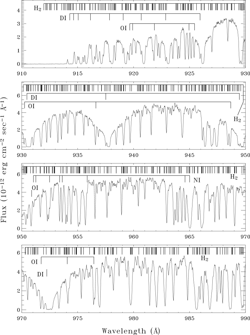
Figure 1.— The SiC1B spectrum of LSE 44. The positions of interstellar D I, O I, N I, and H₂ absorption lines are indicated. Many of the unmarked lines are due to metals arising in the atmosphere of this subdwarf O star. The data have been binned by 2 pixels ($\sim 0.026$ Å) for display purposes only in this figure. Note that the flux scale is not the same on all panels.

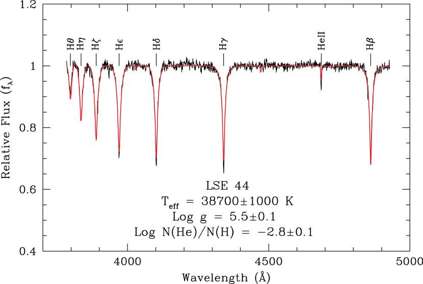
Figure 2.— Black line: normalized optical spectrum of the sdO star LSE 44. Red line: Best model matching the optical spectrum.

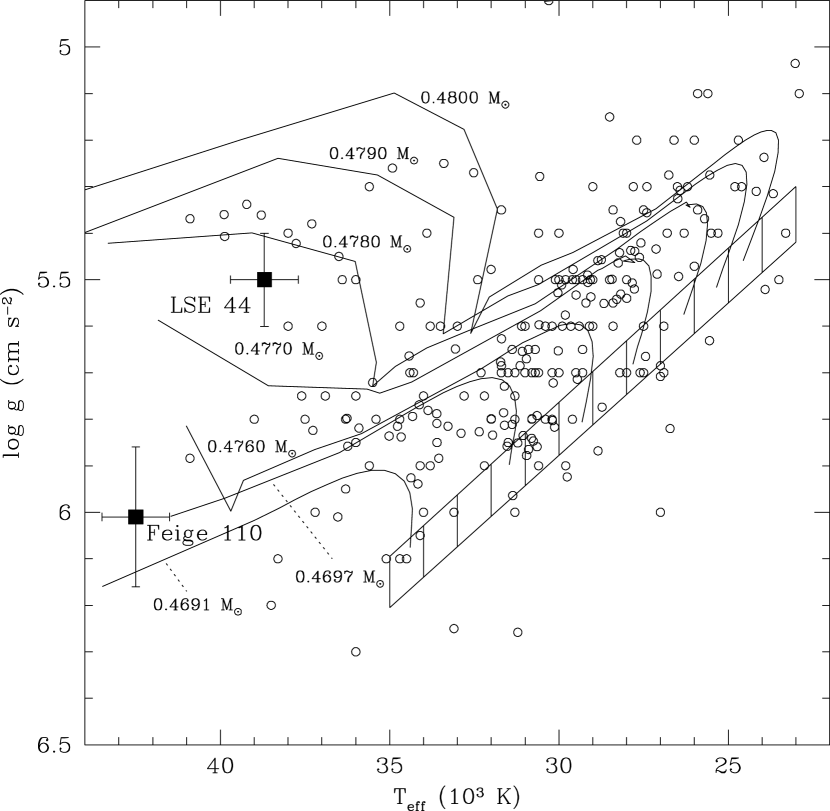
Figure 3.— Position of the sdO star LSE 44 on the $T_{\rm{eff}}$-$g$ plane. Open circles are parameters of observed sdB and sdOB stars. The position of the sdOB star Feige 110 is also indicated (Friedman et al. 2002). Solid lines are post-EHB evolutionary tracks from B. Dorman (1999, private communication). The numbers indicate the mass of a star in solar masses that corresponds to an evolutionary track. The hashed region is the ZAEHB.

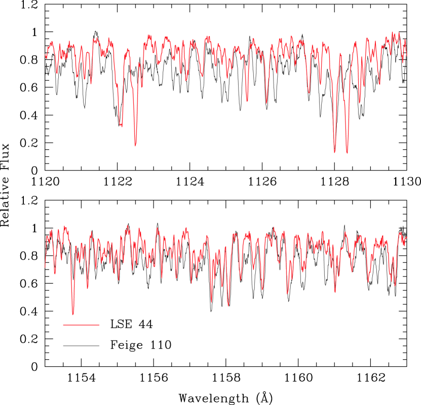
Figure 4.— Portions of the FUSE spectrum of LSE 44 (red line) compared to the FUSE spectrum of the sdOB star Feige 110 (black line). Many unidentified lines appear in spectra of both stars.

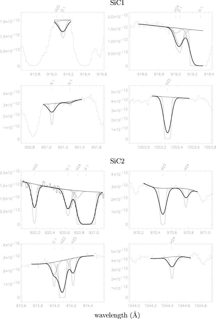
Figure 5.— Examples of spectral windows used in the profile fitting analysis. Histogram lines are the data, heavy black lines are the fits, light black lines are the continua, and the dashed lines are the fits for the individual species. The dotted lines are the model profiles prior to convolution with the LSF. The H₂ lines of levels $J=2$ and $J=5$ are designated as H22 and H25. The X-axis is wavelength in Å and the Y-axis is flux in units of ergs cm^-2 s^-1 Å${}^{-1}.$ Eight spectral windows are displayed here, including 18 transitions. However, the complete fit includes typically 60 spectral windows in all FUSE detector segments, and approximately 100 transitions.

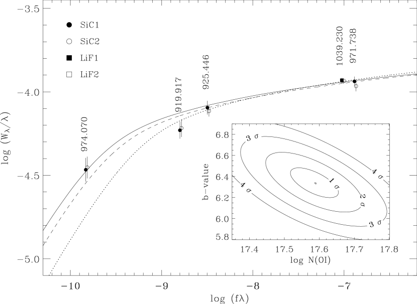
Figure 6.— The single component, Gaussian curve of growth for O I. The best fit solution, which excludes the $\lambda 919$ line, is log $N$(O I) = $17.59^{+0.13}_{-0.14}$ and $b=6.33^{+0.30}_{-0.26}$ (solid line). Including all lines gives log $N$(O I) = $17.52^{+0.22}_{-0.23}$ and $b=6.33^{+0.49}_{-0.44}$ (dashed line). The solution if both the $\lambda 974$ and $\lambda 919$ lines are excluded is log $N$(O I) = $17.22^{+0.55}_{-0.29}$ and $b=6.85^{+0.57}_{-0.75}$ (dotted line), which demonstrates that the lack of optically thin lines can result in a large error in the column density estimate. See §4.2 for additional discussion. For clarity, at each wavelength the data points derived from each of the FUSE channels have been slightly separated. The inset shows the log($N$)/$b-$value error contours for the best fit solution.

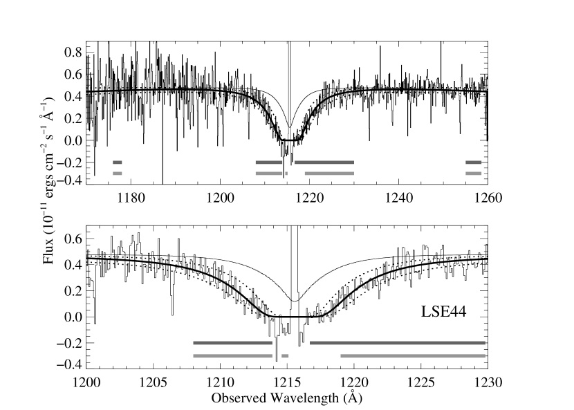
Figure 7.— High-dispersion IUE observation of LSE 44 (histogram) with the best fit H I profile (black line through spectrum) and upper and lower bounds (dotted lines) on $N$(H I) at the $2\,\sigma$ confidence level. The highest curve is the stellar model, described in §3. We have used the spectral region indicated by the dark horizontal line in the fit. Note that this uses the region from approximately $1216.5-1218.1$Å, in the core of the saturated line, to establish the flux zero point. We initially used the spectral region indicated by the gray horizontal line for the fit, but determined that this incorrectly set the zero point of the flux. See §4.4.2 for additional discussion. The upper and lower panels plot the same data and fits on different scales to enable the reader to inspect the details in the Ly$\alpha$ profile as well as the continuum fit well away from the interstellar H I line. The emission line in the center of the saturated Ly$\alpha$ core is geocoronal Ly$\alpha$ emission, and is excluded from the analysis of the interstellar H I column density.

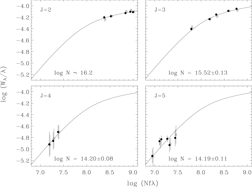
Figure 8.— Curves-of-growth for H₂ $J=2-5$ rotational levels. All curves are ploted over the same range of log (Nf$\lambda$) to clearly display the rotational levels for which $N(H_{2})$ is well-constrained. For $J=2$ it is not possible to detemine a meaningful column density error because all lines are saturated. The $b-$value is well constrained only for $J=3$, for which $b=7.54^{+0.53}_{-0.44}$ km s^-1. We set $b=7.54$ when computing the COG for $J=4$ and $J=5$, although the column densities are insensitive to the choice of $b$. Filled symbols are data from SiC1B channel, and open symbols from SiC2A.

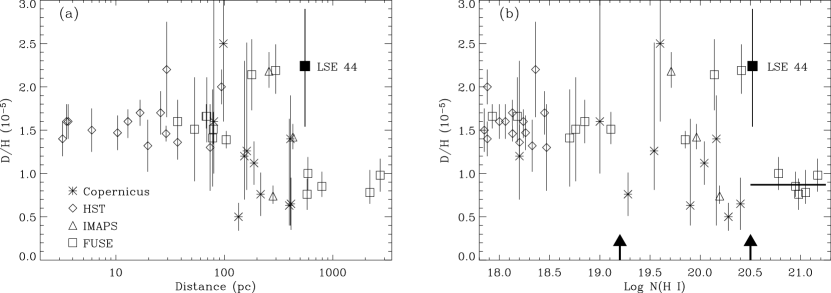
Figure 9.— D/H as a function of (a) distance and (b) H I column density. In this figure, adapted from Wood et al. (2004), the $1\sigma$ errors are plotted. The filled square shows the data point from this study. The arrows in panel (b) indicate the Wood at al. boundary of the Local Bubble, at log $N({\rm H\;\mbox{\small\rm I}})$ = 19.2, and the start of the third D/H regime, at log $N({\rm H\;\mbox{\small\rm I}})$ = 20.5, where D/H is averaged over many regions, leading to a roughly constant value. The horizontal lines indicate the average values of D/H for log $N({\rm H\;\mbox{\small\rm I}})$$<19.2$ and log $N({\rm H\;\mbox{\small\rm I}})$$>20.5$ (excluding LSE 44), respectively. Mixing caused by supernovae may be responsible for the uniform D/H distribution within $\sim 100$ pc. Also included in these plots are results from Williger et al. (2005) and Hébrard et al. (2005).