Mg isotope ratios in giant stars of the globular clusters M 13 and M 71

Abstract

We present Mg isotope ratios in 4 red giants of the globular cluster M 13 and 1 red giant of the globular cluster M 71 based on high resolution, high signal-to-noise ratio spectra obtained with HDS on the Subaru Telescope. We confirm earlier results by Shetrone that for M 13, the ratio varies from ²⁵⁺²⁶Mg/²⁴Mg $\simeq$ 1 in stars with the highest Al abundance to ²⁵⁺²⁶Mg/²⁴Mg $\simeq$ 0.2 in stars with the lowest Al abundance. However, we separate the contributions of all three isotopes and find a considerable spread in the ratio ²⁴Mg:²⁵Mg:²⁶Mg with values ranging from 48:13:39 to 78:11:11. As in NGC 6752, we find a positive correlation between ²⁶Mg and Al, an anticorrelation between ²⁴Mg and Al, and no correlation between ²⁵Mg and Al. In M 71, our one star has a Mg isotope ratio 70:13:17. For both clusters, even the lowest ratios ²⁵Mg/²⁴Mg and ²⁶Mg/²⁴Mg exceed those observed in field stars at the same metallicity, a result also found in NGC 6752. The contribution of ²⁵Mg to the total Mg abundance is constant within a given cluster and between clusters with ²⁵Mg/^24+25+26Mg $\simeq$ 0.13. For M 13 and NGC 6752, the ranges of the Mg isotope ratios are similar and both clusters show the same correlations between Al and Mg isotopes suggesting that the same process is responsible for the abundance variations in these clusters. While existing models fail to reproduce all the observed abundances, we continue to favor the scenario in which two generations of AGB stars produce the observed abundances. A first generation of metal-poor AGB stars pollutes the entire cluster and is responsible for the large ratios of ²⁵Mg/²⁴Mg and ²⁶Mg/²⁴Mg observed in cluster stars with compositions identical to field stars at the same metallicity. Differing degrees of pollution by a second generation of AGB stars of the same metallicity as the cluster provides the star-to-star scatter in Mg isotope ratios.

1 Introduction

For elements heavier than Si, spectroscopic analyses of field stars and globular cluster stars have shown that they have essentially identical chemical abundance ratios [X/Fe] at a given metallicity, [Fe/H] (e.g., see reviews by Gratton et al. 2004 and Sneden et al. 2004a). Yet for the light elements, C-Al, every well studied Galactic globular cluster exhibits star-to-star abundance variations (e.g., see review by Kraft 1994). While the amplitude of the dispersion may differ from cluster to cluster, a common pattern is evident in which anticorrelations are found between the abundances of C and N, O and Na, and Mg and Al. Such variations have never been detected in field stars with comparable ages, metallicities, and evolutionary status (Pilachowski et al., 1996; Hanson et al., 1998). There is still no satisfactory explanation for the origin of the globular cluster abundance variations.

The two explanations for the star-to-star globular cluster composition anomalies, the evolutionary and primordial scenarios, both assume that proton-capture reactions (CNO-cycle, Ne-Na chain, and Mg-Al chain) are responsible for altering the light element abundances. The principal difference is the site in which the nucleosynthesis is thought to occur. In the evolutionary scenario, the observed low-mass red giants are believed to have altered their compositions via internal mixing and nucleosynthesis. To change the surface abundances of O, Na, Mg, and Al requires exposure to very high temperatures through very deep mixing that is not predicted by standard models (e.g., Sweigart & Mengel 1979, Charbonnel 1995, and Fujimoto et al. 1999). In the primordial scenario, the abundance anomalies are believed to be synthesized within intermediate-mass asymptotic giant branch (IM-AGBs) or other stars. The present cluster members either formed from gas contaminated by these stars or accreted such ejecta after formation.

Measurements of the Mg isotope ratios offer a powerful insight into the stars responsible for the abundance variations because the individual isotopes are destroyed at different temperatures within low mass red giants and IM-AGBs. Mg is one of the rare elements for which stellar isotope ratios can be accurately measured. The three stable isotopes are the alpha-nucleus ²⁴Mg and the neutron-rich ²⁵Mg and ²⁶Mg. Mg isotope ratios have been measured in only two globular clusters. Shetrone (1996a, b) analyzed 6 bright giants in M 13 and Yong et al. (2003a) (hereafter Y03) analyzed 20 bright giants in NGC 6752. While both analyses showed that the ratio ²⁵⁺²⁶Mg/²⁴Mg varied within each cluster, Shetrone was unable to separate the contribution of ²⁵Mg from ²⁶Mg. Being able to separate the contribution of each isotope is vital and only possible when analyzing very high resolution spectra. Y03 showed for NGC 6752 that ²⁴Mg and Al are anticorrelated, ²⁵Mg and Al are not correlated, and that ²⁶Mg and Al are correlated. Synthesis of the large Al enhancements via proton capture on ²⁴Mg within the Mg-Al chain is predicted to only occur at very high temperatures such as those found in IM-AGBs of the highest mass at their maximum luminosity (Karakas & Lattanzio, 2003). However, the constancy of ²⁵Mg and the correlation of ²⁶Mg and Al are not predicted from IM-AGB models (Denissenkov & Herwig, 2003; Fenner et al., 2004; Ventura & D’Antona, 2005) which underscores the fact that our present theoretical knowledge of stellar nucleosynthesis and/or globular cluster chemical evolution is incomplete. Additional measurements of Mg isotope ratios in globular clusters are required and it is crucial to distinguish the contributions of all three isotopes.

In this paper, we present measurements of the Mg isotope ratios in four bright red giants of the globular cluster M 13 as well as one bright red giant of the globular cluster M 71. We re-analyze a subset of Shetrone’s M 13 stars and make the important separation of the contributions of ²⁵Mg from ²⁶Mg. M 13, along with NGC 6752, exhibits the largest dispersion in Al abundance of all the well studied Galactic globular clusters. M 13 has a very similar iron abundance to NGC 6752, [Fe/H] $\simeq$ $-$1.5. Previous studies of this cluster include Popper (1947), Arp & Johnson (1955), Helfer et al. (1959), Cohen (1978), Peterson (1980), Kraft et al. (1992), Shetrone (1996a, b), Sneden et al. (2004b), and Cohen & Meléndez (2005). M 71 is a more metal-rich cluster, [Fe/H] $\simeq$ $-$0.8, that displays a mild O-Na anticorrelation and a subtle variation in Al abundance. Previous studies of this cluster include Arp & Hartwick (1971), Cohen (1980), Smith & Norris (1982), Leep et al. (1987), Smith & Penny (1989), Sneden et al. (1994), Ramírez & Cohen (2002, 2003), and Lee et al. (2004).

2 Observations and data reduction

Observations of the four M 13 red giants and the M 71 red giant were obtained with the Subaru Telescope using the High Dispersion Spectrograph (HDS; Noguchi et al. 2002) on 2004 June 1. The comparison field star, HD 141531, was also observed since it is a red giant whose evolutionary status and stellar parameters are comparable to the globular cluster giants. Y03 measured Mg isotope ratios in HD 141531 allowing a comparison between data from Subaru HDS and VLT UVES. A 0.4″ slit was used providing a resolving power of $R=\lambda/\Delta\lambda$=90,000 per 4 pixel resolution element with wavelength coverage from 4000 Å to 6700 Å. The integration times were about 60 minutes per star. The typical signal-to-noise ratio (S/N) for the program stars was 130 per pixel (260 per resolution element) at 5140 Å. One-dimensional wavelength calibrated normalized spectra were produced in the standard way using the IRAF package of programs. In Table 1, we present our list of program stars.

3 Analysis

3.1 Stellar parameters and elemental abundance ratios

We undertook a traditional spectroscopic approach for estimating the stellar parameters: the effective temperature ($T_{\rm eff}$), the surface gravity (log $g$), and the microturbulent velocity ($\xi_{t}$). Equivalent widths (EWs) were measured for a set of Fe i and Fe ii lines using routines in IRAF where in general Gaussian profiles were fitted to the observed profiles. The set of Fe lines were taken from Y03, Biémont et al. (1991), and Blackwell et al. (1995, and references therein). The EWs and atomic data are presented in Table 2. The model atmospheres were taken from the Kurucz (1993) local thermodynamic equilibrium (LTE) stellar atmosphere grid and we used the LTE stellar line analysis program Moog (Sneden, 1973). To set the effective temperature, we adjusted $T_{\rm eff}$ until there was no trend between the abundance from Fe i lines and the lower excitation potential, i.e., excitation equilibrium. For the surface gravity, we adjusted $\log g$ until the abundances from Fe i and Fe ii were equal, i.e., ionization equilibrium. Finally, the microturbulent velocity was set by the requirement that the abundances from Fe i lines shows no trend with EW. The final [Fe/H] was taken to be the mean of all Fe lines assuming a solar abundance log $\epsilon$(Fe) = 7.50. In Table 1 we present our derived stellar parameters for the program stars.

For HD 141531, we compared the EWs for Fe i and Fe ii lines and found an excellent agreement between the Subaru (this study) and the VLT (Y03) measurements. Therefore, we adopted the same stellar parameters for HD 141531 as used in Y03. We estimate the internal errors in the stellar parameters to be $T_{\rm eff}$ $\pm$ 50, $\log g~{}\pm$ 0.2, and $\xi_{t}~{}\pm$ 0.2. Within these uncertainties, our stellar parameters for the M 13 giants compare very well with those derived by Shetrone (1996a, b), Sneden et al. (2004b), and Cohen & Meléndez (2005). For M 71 A4, our stellar parameters agree very well with those derived by Sneden et al. (1994) and Shetrone (1996a, b). (See Table Mg isotope ratios in giant stars of the globular clusters M 13 and M 71 for comparison of stellar parameters.)

We also measured abundances for O, Na, Mg, and Al using the same lines presented in Y03 (atomic data and EWs are presented in Table 2). In Table 4 we present the abundance ratios [Fe/H] and [X/Fe] for the program stars assuming solar abudances of 8.69, 6.33, 7.58, and 6.47 for O, Na, Mg, and Al respectively. In this table, we also compare our abundance ratios with previous studies of these stars, namely Sneden et al. (1994, 2004b), Shetrone (1996a, b), and Cohen & Meléndez (2005). In general, the abundance ratios are in good agreement with previous determinations. However, for [O/Fe] our two measurements do not agree with those derived by Sneden et al. (2004b). (We note that they reference the O abundances to Fe ii and that in some cases there is a difference between the abundances from neutral and ionized iron.) To ensure consistency with their previous studies on globular clusters, Sneden et al. (2004b) adopt the “traditional” solar oxygen abundance log $\epsilon$(O) = 8.93 (Anders & Grevesse, 1989) rather than the revised value of 8.69 recommended by Allende Prieto et al. (2001). The adopted solar oxygen abundance accounts for the offset between our abundances and those of Sneden et al. (2004b). Similarly, Shetrone used the traditional solar oxygen abundance which explains the difference in derived abundances. Cohen & Meléndez (2005) find different abundances for M 13 L70 (II-67) which cannot be attributed to the adopted solar abundances or stellar parameters. We note that they find a 0.3 dex discrepancy between Fe i and Fe ii. In Table 5, we present the abundance dependences upon the model parameters.

3.2 Mg isotope ratios

The first measurements of stellar Mg isotope ratios were performed by Boesgaard (1968) who examined the 0-0 band of the A-X electronic transition of the MgH molecule. As a result of the isotopic wavelength splitting, ²⁵MgH and ²⁶MgH contribute a red asymmetry to the main ²⁴MgH line (see Figure 1). Subsequent studies have also exploited the molecular MgH lines to measure Mg isotope ratios in cool dwarfs and giants (e.g., Tomkin & Lambert 1976, 1979, 1980, Barbuy 1985, 1987, Barbuy et al. 1987, Lambert & McWilliam 1986, McWilliam & Lambert 1988, Gay & Lambert 2000, Yong et al. 2003b, 2004 and references therein). Pre-solar grains allow measurements of Mg isotope ratios with exquisite precision and offer a powerful additional insight into stellar nucleosynthesis (e.g., Nittler et al. 2003 and Clayton & Nittler 2004).

Inspection of Figure 1 shows that the profiles of the MgH lines are asymmetric with ²⁵MgH and ²⁶MgH providing red wings. This figure also shows that the profiles of the MgH lines differ significantly among the M 13 giants. In particular, M 13 L973 and M 13 L70 appear to have substantial contributions of ²⁶MgH relative to M 13 L 629 and M 13 L 598. M 71 A4 also exhibits an asymmetric profile suggesting a large contribution from ²⁶MgH. While we can gain a qualitative appreciation that the Mg isotope ratios vary within M 13 by looking at the spectra, spectrum synthesis is necessary to measure accurate ratios. Next we describe our approach which is identical to Gay & Lambert (2000), Y03, and Yong et al. (2003b, 2004).

Numerous lines from the A-X electronic transition of the MgH molecule are present in the spectra of these cool red giants. However, few of these lines offer a reliable measure of the Mg isotope ratios due to the presence of known and unknown blends. McWilliam & Lambert (1988) recommended 3 lines from which accurate isotope ratios can be extracted. The first line at 5134.6 Å is due to the $Q_{1}(23)$ and $R_{2}(11)$ lines from the 0-0 band. The weaker MgH features on either side of the 5134.6 Å line are contaminated such that reliable isotope ratios cannot be measured (Tomkin & Lambert, 1980). The second line at 5138.7 Å is a blend of the 0-0 $Q_{1}(22)$ and 1-1 $Q_{2}(14)$ MgH lines. The third line at 5140.2 Å is a blend of the 0-0 $R_{1}(10)$ and 1-1 $R_{2}(4)$ MgH lines. We refer to these lines as Region 1, Region 2, and Region 3 respectively.

To measure the Mg isotope ratios, we generated synthetic spectra using Moog. The macroturbulent broadening was assumed to have a Gaussian form and was estimated by fitting the profiles of the Ni i line at 5115.4 Å and the Ti i line at 5145.5 Å. These clean atomic lines were slightly stronger than the three recommended MgH lines. These lines gave the same macroturbulence within 1.0 km s^-1 and the smaller value was adopted if there was a disagreement. Our list of atomic and molecular lines was identical to the Gay & Lambert (2000) list and includes the contributions from C, Mg, Sc, Ti, Cr, Fe, Co, Ni, and Y. For the MgH isotopic components, the wavelengths were taken from McWilliam & Lambert (1988) and were based on direct measurements of an MgH spectrum obtained using a Fourier transform spectrometer by Bernath et al. (1985).

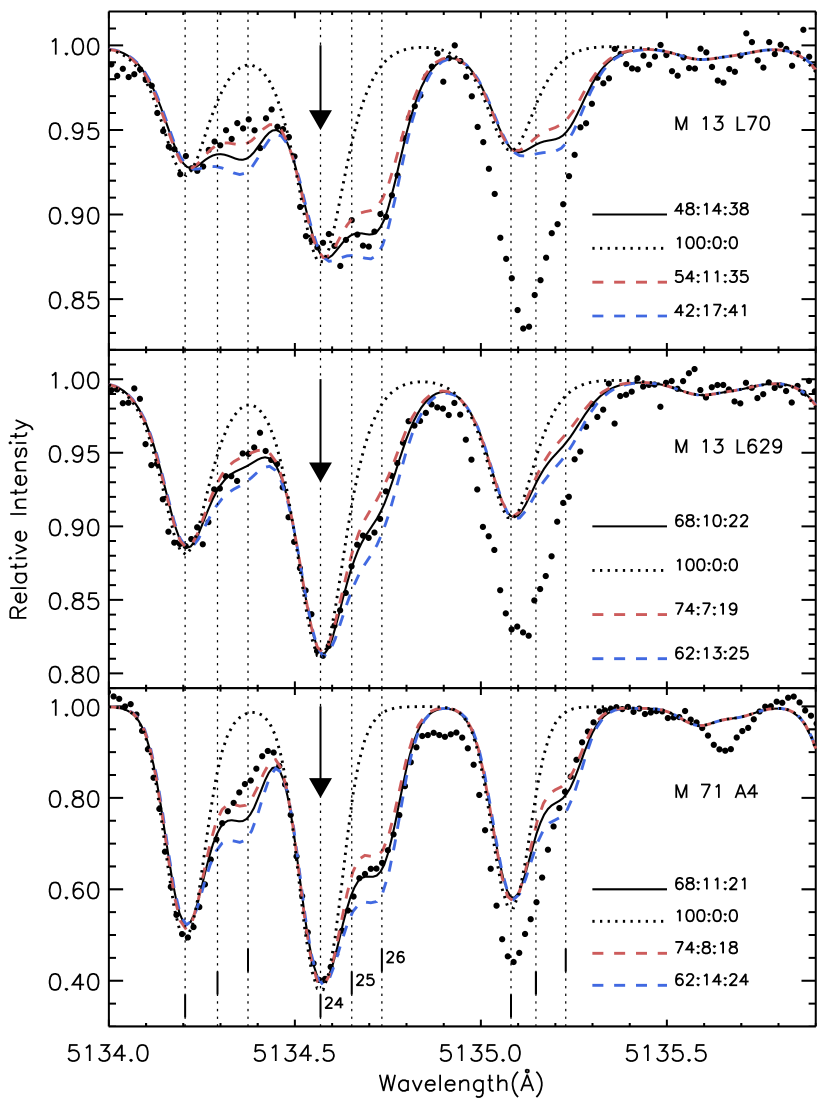
Figure 2: Spectra of M 13 L70, M 13 L629, and M 71 A4 for Region 1. The feature we are fitting is highlighted by the black arrow. The positions of ²⁴MgH, ²⁵MgH, and ²⁶MgH are marked by dashed lines. Filled circles represent the observed spectra, the best fit is the solid line, and unsatisfactory ratios are also shown.

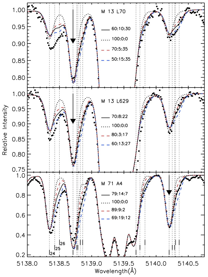
Figure 3: Spectra of M 13 L70, M 13 L629, and M 71 A4 for Regions 2 and 3. The feature we are fitting is highlighted by the black arrow. The positions of ²⁴MgH, ²⁵MgH, and ²⁶MgH are marked by dashed lines. Filled circles represent the observed spectra, the best fit is the solid line, and unsatisfactory ratios are also shown.

Treating each recommended line independently, we adjusted the isotope ratios and Mg abundance until the profile was best fit. Following Nissen et al. (1999, 2000) who measured Li isotope ratios, we chose to use a $\chi^{2}$ analysis to determine the best fit to the data. The advantages are that this method is unbiased and allows us to quantify the errors to the fits. The free parameters were (1) ²⁵Mg/²⁴Mg, (2) ²⁶Mg/²⁴Mg, and (3) the Mg abundance, log $\epsilon$(Mg). Our initial guess was the best fit as determined by eye. We explored a large volume of parameter space around the initial estimate and calculated $\chi^{2}=\Sigma(O_{i}-S_{i})^{2}/\sigma^{2}$ where $O_{i}$ is the observed spectrum point, $S_{i}$ is the synthesis, and $\sigma=(S/N)^{-1}$. Optimum values were determined by locating the $\chi^{2}$ minima for each free parameter ²⁵Mg/²⁴Mg, ²⁶Mg/²⁴Mg, and log $\epsilon$(Mg). We then used a more refined grid and searched a smaller volume in parameter space centered upon the optimum value. For each region in each star, we generated and tested over 500 synthetic spectra. Throughout the various iterations for each region in each star, the optimal isotope ratio always converged to a similar value. The best fit as determined by eye was always similar to the best fit as determined via the $\chi^{2}$ analysis. In Figures 2 and 3, we show examples of the best fitting synthetic spectra.

Following Bevington & Robinson (1992) and Nissen et al. (1999, 2000), we plot $\Delta\chi^{2}=\chi^{2}-\chi^{2}_{min}$ for the ratios ²⁵Mg/²⁴Mg and ²⁶Mg/²⁴Mg (see Figure 4). The $\Delta\chi^{2}=1$ represents the corresponding 1$\sigma$ confidence limit for determining ²⁵Mg/²⁴Mg or ²⁶Mg/²⁴Mg. For each recommended line in each star, we paired an uncertainty to the optimized ratio ²⁵Mg/²⁴Mg or ²⁶Mg/²⁴Mg. The final ratio ²⁴Mg:²⁵Mg:²⁶Mg was calculated based on the weighted mean. As noted in previous investigations of Mg isotope ratios, the ratio ²⁵Mg/²⁴Mg is less certain than ²⁶Mg/²⁴Mg since ²⁶MgH is less blended with the strong ²⁴MgH line. Furthermore, isotope ratios for Regions 2 and 3 are less accurate than for Region 1. Although we calculated the formal statistical errors, these numbers are small and ignore systematic errors such as continuum fitting, macroturbulence, and blends. Figures 2 and 3 show that the uncertainties in the ratios are probably at or below the level b $\pm$ 5 or c $\pm$ 5 when expressing the ratio as ²⁴Mg:²⁵Mg:²⁶Mg=(100$-$b$-$c):b:c. For Region 1 in M 13 L 70, when we lower the continuum level by 1%, the best fitting ratio is 49:11:40 (originally 48:14:38). When we change the macroturbulence from 7.5 km s^-1 to 8.0 km s^-1, the best fitting ratio is 48:14:38. For Region 2 in M 13 L598, when we lower the continuum by 1% and change the macroturbulence from 6.5 km s^-1 to 7.0 km s^-1, we measure ratios of 81:6:13 and 84:9:7 respectively (originally 80:10:10). Note that the derived isotope ratios are insensitive to the adopted stellar parameters and appear immune to non-LTE effects and/or inadequacies in the model atmospheres (Yong et al., 2003b, 2004).

In Table 6 we present the Mg isotope ratios for the program stars. In this table we also compare our values with previous determinations. Our superior data, higher S/N and higher spectral resolution, confirm the pioneering results obtained by Shetrone. While Shetrone (1996b) was unable to distinguish between ²⁵Mg and ²⁶Mg, we note that our ratios ²⁵⁺²⁶Mg/²⁴Mg are in excellent agreement. For the comparison field star, HD 141531, the isotope ratio measured from the Subaru data is in excellent agreement with the value from the VLT data.

In the spectra of dwarfs, previous studies of Mg isotope ratios (e.g., Gay & Lambert 2000; Yong et al. 2003b, 2004) show that the best fitting synthesis to the 5134.6 Å line generally predicts a weaker 5134.2 Å line than is observed. (As mentioned earlier, Tomkin & Lambert (1980) showed that the 5134.2 Å line does not provide a reliable isotope ratio.) In some cases, the predicted strength of 5134.2 Å is very close to the observed strength. For cases in which the synthetic spectra underpredict the observed strength, a weak line not included in the line list could account for the small mismatch. However in giants, the mismatch appears to be in the opposite direction. As shown in Figure 2, the synthetic spectra overpredict the strength of the MgH 5134.2 Å line. Our linelist includes lines of C₂ at 5134.3 and 5134.7 Å. Our estimate of the C abundance was based on the weak C₂ lines near 5135.6 Å which gave [C/Fe] $\simeq$ $-$0.2. Even if we exclude the C₂ lines at 5134.3 and 5134.7 Å, the syntheses continue to overpredict the strength of the 5134.2 Å line.

On closer inspection of the NGC 6752 giants, we note that the magnitude of the mismatch appears to be a function of luminosity with the discrepancy being largest at the tip of the RGB ($T_{\rm eff}$ $\simeq$ 3900K) and disappearing by $T_{\rm eff}$ $\simeq$ 4400K. Our M 13 and M 71 giants are all located at the tip of the RGB where the discrepancy reaches a maximum. We note that a best fit to the 5134.2 Å line could be achieved with a reduced amount of ²⁶Mg relative to the 5134.6 Å line. However, substantial amounts of ²⁵Mg and ²⁶Mg would still be required.

4 Discussion

4.1 Elemental abundance ratios in M 13

First we will focus upon M 13 since our sample for M 71 consists of only 1 star. Of the elemental abundance ratios that we have measured, [Al/Fe] exhibits the largest amplitude. Though we have only observed 4 giants, the [Al/Fe] ratios vary by more than an order of magnitude (1.04 dex). This variation far exceeds the measurement uncertainty. As a comparison, Sneden et al. (2004a) measured Al abundances in a sample of 18 bright giants. Excluding the 2 stars for which only upper limits are available, the ratio [Al/Fe] varies by roughly 1.2 dex. Therefore, our 4 stars span almost the full range of the star-to-star abundance variation for [Al/Fe]. Our most Al-rich star, M 13 L973, is also one of the most Al-rich stars in the Sneden sample. However, our most Al-poor star, M 13 L598, is still roughly 0.2 dex more Al-rich than the most Al-poor star in the Sneden sample. Our ratios of [Na/Fe] vary by almost a factor of 3 (0.47 dex) which again greatly exceeds the measurement uncertainty. Sneden et al. (2004a) measured Na abundances in 35 bright giants and found the ratio [Na/Fe] varies by 0.95 dex. Our ratios of [Mg/Fe] vary by a factor of two (0.28 dex) which is greater than the measurement uncertainty. Sneden et al. (2004a) measured [Mg/Fe] in 18 stars and found the ratio varies by 0.57 dex. Comparing the dispersion in our [Na/Fe] and [Mg/Fe] ratios with the Sneden sample, our stars span a considerable range of the abundance distribution. However, Sneden’s M 13 sample contains several stars that are more enhanced in Na and Mg as well as several that are more depleted in Na and Mg. Even within our small sample, we recover the Mg-Al anticorrelation and find that Na is correlated with Al in accord with previous studies of this cluster.

4.2 Mg isotope ratios in M 13

For M 13, we confirm Shetrone’s finding that the ratio ²⁴Mg:²⁵Mg:²⁶Mg varies considerably from star to star. Our measured ratios ²⁵⁺²⁶Mg/²⁴Mg are very similar to those measured by Shetrone. We find that the lowest ratio is 78:11:11 while the highest ratio is 48:13:39. Note that the lowest observed ratio in NGC 6752 was 84:8:8 and the highest observed ratio was 53:9:39. Although the M 13 sample is limited, the extremes in the isotope ratios appear to have similar values as for NGC 6752. Shetrone (1996b) measured Mg isotope ratios in 6 stars and based on these values, we made sure that we observed the stars exhibiting the lowest (M 13 L598) and highest (M 13 L70) isotope ratios.

In M 13 L598, the star with the lowest ratio, we find equal contributions from ²⁵Mg and ²⁶Mg such that ²⁵Mg = ²⁶Mg or equivalently, ²⁵Mg/²⁴Mg = ²⁶Mg/²⁴Mg. In NGC 6752, we also found a similar result with ²⁵Mg $\simeq$ ²⁶Mg in stars with low isotope ratios. For the remaining stars in M 13, we do not find ²⁵Mg = ²⁶Mg. Instead, the contribution from ²⁶Mg exceeds that from ²⁵Mg. Such a result would again appear to be similar to NGC 6752. Another aspect of the Mg isotope ratios common to both M 13 and NGC 6752 is that the contribution of ²⁵Mg to the total Mg abundance is essentially constant from star-to-star with ²⁵Mg/^24+25+26Mg $\simeq$ 0.13. The isotope ratio ²⁴Mg:²⁵Mg:²⁶Mg varies due to the changing contributions of ²⁴Mg and ²⁶Mg, i.e., ²⁴Mg/^24+25+26Mg and ²⁶Mg/^24+25+26Mg differ from star-to-star in NGC 6752 and M 13.

In Y03, we noted that at one extreme of the star-to-star abundance variations are stars whose compositions [O/Fe], [Na/Fe], [Mg/Fe], and [Al/Fe] are essentially identical to field stars at the same metallicity, [Fe/H]. These are the stars with high O, high Mg, low Na, and low Al and we refer to them as “normal stars”. At the other extreme of the abundance variations are the stars with high Na, high Al, low O, and low Mg. We referred to these stars as “polluted” in anticipation that proton capture nucleosynthesis can produce O-poor, Na-rich, Mg-poor, and Al-rich gas. The pollution may have occurred via either the evolutionary or primordial scenario. Figure 13.8 in Sneden et al. (2004a) shows the O-Na anticorrelation and the Na-Al correlation. In this Figure, the field stars clearly occupy one end of the distribution defined by the cluster stars, i.e., the region in which the “normal” cluster stars are located. This Figure, and other large samples of field giants, confirm that our single comparison star HD 141531 is representative of field stars.

Theoretical yields from metal-poor supernovae predict very small amounts of ²⁵Mg and ²⁶Mg relative to ²⁴Mg, e.g., ²⁴Mg:²⁵Mg:²⁶Mg $\simeq$ 98:1:1 (Woosley & Weaver, 1995; Chieffi & Limongi, 2004). Based on these yields, Galactic chemical evolution models predict ²⁴Mg:²⁵Mg:²⁶Mg $\simeq$ 98:1:1 in the range $-4<$ [Fe/H] $<-1$ (Timmes et al., 1995; Goswami & Prantzos, 2000; Alibés et al., 2001). We stress that in calculating these predictions, the isotopes of Mg are assumed to be synthesized solely by Type II supernovae. The “normal” stars in NGC 6752 had ratios of ²⁵Mg/²⁴Mg and ²⁶Mg/²⁴Mg that exceeded predictions from metal-poor supernovae as well as the ratios observed in field stars at the same metallicity (e.g., Gay & Lambert 2000 and Yong et al. 2003b). Applying the same criteria, M 13 L598 would be a “normal” star whereas M 13 L629, M 13 L973, and M 13 L70 are “polluted” with L70 being the most “polluted”. Again, we find that the Mg isotope ratios in M 13 parallel those found in NGC 6752. The “normal” star M 13 L598 has a Mg isotope ratio ²⁴Mg:²⁵Mg:²⁶Mg = 78:11:11 that exceeds predictions by an order of magnitude and these isotope ratios also exceed field stars at the same metallicity. At the metallicity of M 13, a typical field halo star such as Gmb 1830 (a subdwarf) has ²⁴Mg:²⁵Mg:²⁶Mg = 94:3:3 (Tomkin & Lambert, 1980). Our comparison field star, HD 141531, has a ratio 91:4:6. In NGC 6752 and M 13, we find that “normal” stars have isotope ratios of Mg that differ from field stars at the same metallicity despite the similarity in elemental abundance ratios [O/Fe], [Na/Fe], [Mg/Fe], and [Al/Fe].

4.3 Mg isotopic abundances in M 13

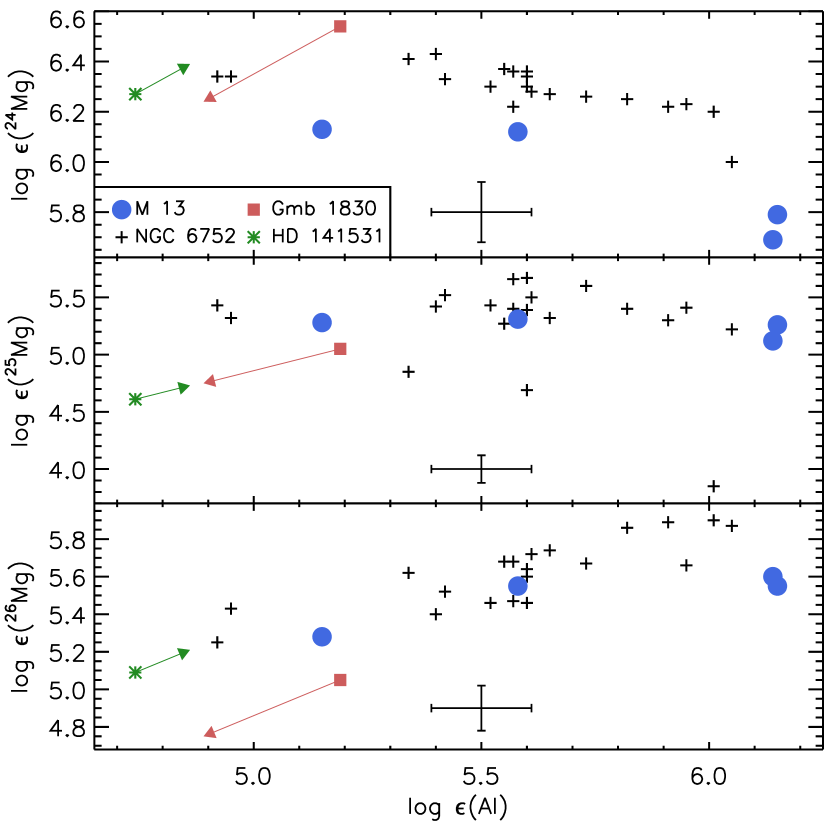
Figure 5: The abundances of ²⁴Mg, ²⁵Mg, and ²⁶Mg versus Al. The filled blue circles represent M 13 while the black plus signs represent NGC 6752 (Y03). The field stars Gmb 1830 (filled red square: Mg isotope ratio from Tomkin & Lambert 1980 and abundance ratios from Fulbright 2000) and HD 141531 (green asterisk) are overplotted. A representative error bar is shown in each panel. The arrows show the field star abundances if we adjust for the metallicity differences between M 13 and the field stars assuming that $\Delta\log~{}\epsilon$(species) = $\Delta\log~{}\epsilon$(Fe).

In Figure 5, we plot the Mg isotopic abundances versus the Al abundance. The Mg isotopic abundances were derived by combining the Mg isotope ratios from molecular MgH lines with the Mg elemental abundance from Mg i lines. We note that the ²⁴Mg abundance decreases with increasing Al abundance and that the total spread in the ²⁴Mg abundance is a factor of 2.75 which is greater than the measurement uncertainty. The ²⁵Mg abundance appears constant over the 1.0 dex range in [Al/Fe]. The ²⁶Mg abundance increases with increasing Al abundance. The total dispersion in the ²⁶Mg abundance is a factor of 2.1 which exceeds the measurement uncertainty. In Figure 5 we overplot the results for NGC 6752. For M 13 and NGC 6752, an identical behavior is found between the Mg isotopic abundances and Al abundance. For both clusters, ²⁴Mg is anticorrelated with Al, ²⁵Mg is not correlated with Al, and ²⁶Mg is correlated with Al.

In this Figure, we also include the abundances for the comparison field star HD 141531 and the well studied subdwarf Gmb 1830. (For Gmb 1830 we took the Mg isotope ratio from Tomkin & Lambert 1980 and the Mg and Al elemental abundances from Fulbright 2000.) If we adjust the abundances for the small metallicity differences between M 13 and the field stars assuming $\Delta\log~{}\epsilon$(species) = $\Delta\log~{}\epsilon$(Fe), the field stars have essentially identical Mg isotopic abundances and Al elemental abundances. With or without this metallicity correction, the field stars clearly lie at one end of the isotopic distribution defined by the cluster stars as previously seen in NGC 6752. In Figure 5, we can also see that the globular clusters have higher isotopic abundances for ²⁵Mg and ²⁶Mg relative to field stars at the same Al abundance.

4.4 Elemental abundance ratios and Mg isotope ratios in M 71

For M 71, our measurements of Mg isotope ratios and elemental abundances are restricted to a single star. Sneden et al. (1994) found evidence for a variation of O and Na in a sample of 10 stars, though it was not clear whether there was an O-Na anticorrelation. Ramírez & Cohen (2003) observed a larger sample of stars and found a clear O-Na anticorrelation and evidence for a variation in the Al abundance for this cluster. Our observed star, M 71 A4, was observed by Sneden et al. (1994) and had one of the higher O abundances though its Na abundance was in the middle of the distribution. Unfortunately, this star was not observed by Ramírez & Cohen (2003). Based on the O abundances measured by Sneden, this star may be a “normal” star but the situation is not clear.

The Mg isotope ratio in M 71 A4 is ²⁴Mg:²⁵Mg:²⁶Mg = 70:13:17. Note that ²⁶Mg/²⁵Mg $>$ 1 and such a ratio does not agree perfectly with the “normal” stars in NGC 6752 and M 13 which tend to have ²⁵Mg = ²⁶Mg. Therefore we tentatively suggest that this star is slightly “polluted” based on the O and Na elemental abundances as well as the Mg isotope ratio. For this star, we again find that the ratios ²⁵Mg/²⁴Mg and ²⁶Mg/²⁴Mg exceed those observed in field stars of comparable metallicity. Finally, we note that the contribution of ²⁵Mg to the total Mg abundance is similar to NGC 6752 and M 13 with ²⁵Mg/^24+25+26Mg = 0.13.

If we assume that the ratio ²⁵Mg/^24+25+26Mg in M 71 A4 is representative of all stars in this cluster (a constant ratio for all stars was found in the larger samples in M 13 and NGC 6572), then such a ratio may be regarded as unusual. The observed and predicted ratio ²⁵Mg/^24+25+26Mg increases with increasing metallicity (Timmes et al., 1995; Gay & Lambert, 2000; Goswami & Prantzos, 2000; Alibés et al., 2001; Yong et al., 2003b). Even if this ratio in globular clusters exceeds field stars at the same metallicity, we may expect that in globular clusters the ratio would also increase with increasing metallicity. Instead, it seems that the ratio ²⁵Mg/^24+25+26Mg does not differ between M 13, NGC 6752, and M 71 despite the iron abundance changing from [Fe/H] = $-$1.6 to [Fe/H] = $-$0.9 as well as the large dispersions in O-Al abundances. Clearly the analyses of additional stars within this cluster (and clusters with different metallicities) are necessary to determine whether there is a spread in the isotope ratio, ²⁴Mg is anticorrelated with Al and/or O, ²⁵Mg is not correlated with O, ²⁶Mg is correlated with O, and if the lowest isotope ratios exceed field stars at the same metallicity.

4.5 Implications for globular cluster chemical evolution

Shetrone (1996b) provided the first measurements of Mg isotope ratios in a globular cluster. His results for M 13 showed that the ratio ²⁵⁺²⁶Mg/²⁴Mg varied from star-to-star. Of great interest was his discovery that the abundant ²⁴Mg decreases with increasing Al abundance. Very high temperatures are necessary for proton-capture on ²⁴Mg. Shetrone proposed a deep-mixing sequence in which Li begins to be destroyed at 10 $\times~{}10^{6}$ K. At 20 $\times~{}10^{6}$ K, C begins to decrease, N increases, and the ratio ¹²C/¹³C decreases. At 30 $\times~{}10^{6}$ K, O begins to decrease, Na begins to increase, and C and N continue fall and rise respectively. The Al abundance increases slightly due to destruction of ²⁵Mg and ²⁶Mg at 40 $\times~{}10^{6}$ K. Finally, Al increases significantly as ²⁴Mg decreases at 70 $\times~{}10^{6}$ K. Based on Shetrone’s isotope ratios (and measurements of other elemental abundance ratios), various schemes were explored in which the abundance variations could be produced through the evolutionary scenario, the primordial scenario, and combinations of the two (e.g., Langer et al. 1997, Denissenkov et al. 1997, 1998, and Weiss et al. 2000).

Observations by Gratton et al. (2001) showed that the anticorrelations of O-Na and Mg-Al exist even in main sequence stars and early subgiants in NGC 6752. Subsequent measurements have shown a similar result for M 71 (Ramírez & Cohen, 2003) and M 13 (Cohen & Meléndez, 2005). The range and amplitude of the abundance variations of O-Al do not vary from the main sequence to the tip of the red giant branch within a given cluster. This behavior differs from the measurements of C and N abundances that vary with evolutionary status (Suntzeff & Smith, 1991). Al variations in unevolved stars demonstrate that the abundance variations cannot be due primarily to internal mixing and nucleosynthesis because main sequence stars and early subgiants have internal temperatures too low to run the Ne-Na or Mg-Al chains. Therefore, the present cluster members must have formed from inhomogeneous gas or accreted such material.

Measurements of Mg isotope ratios in NGC 6752 led Y03 to suggest a revised primordial scenario involving two generations of IM-AGBs. “Normal stars” showed Mg isotope ratios that exceeded both the predictions from metal-poor supernovae as well as the ratios observed in field stars at the same metallicity. Y03 suggested that a prior generation of metal-poor IM-AGBs can raise the low amounts of ²⁵Mg and ²⁶Mg provided by metal-poor supernovae to the much higher levels observed in the “normal” stars. In order to preserve the highly uniform abundances of Fe, Ca, Ni, etc (Yong et al., 2005), the ejecta from these metal-poor IM-AGBs must be thoroughly mixed with the ejecta from metal-poor supernovae prior to the formation of the present cluster members. As seen in Shetrone’s M 13 sample, the large Al enhancement was accompanied by a decrease in ²⁴Mg for the NGC 6752 giants. Destruction of ²⁴Mg only takes place at very high temperatures such as in AGB stars of the highest mass. Y03 suggested that IM-AGBs pollute the environment from which the present generation of stars formed, an idea first proposed by Cottrell & Da Costa (1981). In IM-AGBs, hydrogen-burning at the base of the convective envelope, so-called hot bottom burning (HBB), may produce the observed C to Al abundance patterns. Y03 also showed that the Fe abundance was identical in all stars within the measurement error. So the source of the pollutants must have the same Fe abundance as the present generation of stars. The O abundance varied by nearly an order of magnitude within NGC 6752. In the event that the pollutants contain no O, then the factor of 10 decrease in the O abundance of the most “polluted” stars relative to the “normal” stars is only possible via a mix of 90% pollutants to 10% normal material. In addition to the dominant primordial component, an evolutionary component is essential to account for the C (Suntzeff & Smith, 1991) and Li (Grundahl et al., 2002) destruction with increasing luminosity.

In M 13, we find that stars with elemental abundance ratios in agreement with field stars at the same metallicity, i.e., “normal” stars, have Mg isotope ratios that exceed those seen in field stars. A similar result was seen in NGC 6752. Therefore, we reiterate the suggestion from Y03 that a prior generation of metal-poor IM-AGBs are needed to produce the high ²⁵Mg/²⁴Mg and ²⁶Mg/²⁴Mg seen in “normal” stars of M 13 and NGC 6752.

The principal result of this study is that the neutron-rich Mg isotopes do not necessarily have the same abundance in M 13, i.e., ²⁵Mg/²⁴Mg $\neq$ ²⁶Mg/²⁴Mg. Instead, the isotopic abundance of ²⁵Mg is constant across the 1.0 dex range in Al while the isotopic abundance of ²⁶Mg is correlated with Al. We also confirm Shetrone’s result that ²⁴Mg decreases with increasing Al abundance. These results for M 13 are identical to the behavior of the Mg isotopic abundances in NGC 6752 suggesting that the same mechanism is responsible for the isotopic and elemental abundance variations seen in both clusters. That is, two generations of IM-AGB stars pollute the cluster as just described.

The similarity in the correlations between Mg isotopes and Al abundances in M 13 and NGC 6752 may be regarded as surprising. If the Al variations arise from the IM-AGBs, then it may be reasonable to expect a large cluster-to-cluster variation of the pollution from such stars. Therefore an additional aspect to the IM-AGB scenario may be required. Perhaps the IM-AGBs were of a very similar mass in both clusters.

For M 71, our one star has a Mg isotope ratio ²⁴Mg:²⁵Mg:²⁶Mg = 70:13:17, i.e., ²⁵Mg/²⁴Mg $\neq$ ²⁶Mg/²⁴Mg. We also note that ²⁶Mg/²⁵Mg $>$ 1, a ratio that is always seen in the “polluted” stars of M 13 and NGC 6752. For this star, we find ²⁵Mg/^24+25+26Mg = 0.13 and such a ratio was also seen in every star in M 13 and NGC 6752. M 71 A4 has ratios ²⁵Mg/²⁴Mg and ²⁶Mg/²⁴Mg that exceed field stars at the same metallicity. Such a difference may again be interpreted as resulting from the pollution of the proto-cluster gas by a prior generation of metal-poor IM-AGBs. Clearly additional measurements of Mg isotope ratios in O-rich and O-poor stars in M 71 are required to see if the Mg isotope ratio varies from star to star, the Mg isotopic abundances are correlated with O, and if the contribution of ²⁵Mg to the total Mg abundance is constant. We speculate that the highest ratios of ²⁶Mg/²⁴Mg in M 71 will not be as extreme as those seen in M 13 and NGC 6752 since the amplitude of the Al variation in M 71 is smaller.

If differing degrees of pollution from IM-AGBs of the same generation as the present cluster members is the correct mechanism for producing the O-Al abundance variations, then Fluorine may be expected to exhibit a star-to-star abundance variation. During HBB in IM-AGBs, destruction of F is predicted in AGB models of the highest mass (Lattanzio et al., 2004). Recently, Smith et al. (2005) showed that F varied from star-to-star in M 4 and that the F abundance was correlated with O and anticorrelated with Na and Al. Such variations of F lend further support to the AGB pollution scenario.

While the AGB pollution scenario offers a plausible qualitative explanation for the light element abundance anomalies, quantitative tests reveal several problems. The observed ratios of ²⁵Mg/²⁴Mg and ²⁶Mg/²⁴Mg in stars with O depletions are significantly lower than predictions from AGB models (Denissenkov & Herwig, 2003). The low C and O abundances and high N cannot be produced in AGB models (Denissenkov & Weiss, 2004). In the detailed globular cluster chemical evolution model by Fenner et al. (2004), O was not depleted, Mg was produced rather than destroyed, C+N+O was not constant, and ²⁵Mg should be correlated with ²⁶Mg. These inconsistencies between the observed and predicted compositions highlight that our understanding of stellar nucleosynthesis and globular cluster chemical evolution are incomplete. While the details are model dependent, Busso et al. (2001) suggest that metal-poor IM-AGBs may run the $s$-process. Yong et al. (2005) found evidence for slight abundance variations for Y, Zr, and Ba with each element showing a statistically significant but small correlation with Al. Therefore, the stars responsible for the synthesis of the Al anomalies may have also run the $s$-process. Indeed, Ventura & D’Antona (2005) caution that the choice of mass-loss rates and treatment of convection greatly affect the calculated AGB yields to such an extent that the predictive power of the AGB models is limited.

New constraints on the source of the abundance anomalies have come from observations of Li in main sequence stars in NGC 6752. Pasquini et al. (2005) have shown that Li is correlated with O and anticorrelated with Na in these unevolved stars. Such a behavior is expected given that the Ne-Na cycle operates at temperatures far exceeding those required to destroy Li. Pasquini et al. (2005) emphasize that Li is observed in even the most “polluted” stars with log $\epsilon$(Li) $\simeq$ 2.0, an amount only 2-3 times lower than in stars with the highest Li abundance. Since O and Na vary by roughly an order of magnitude, this implies that Li must also have been synthesized by the stars responsible for the abundance variations. While Pasquini et al. (2005) also recognize that the yields from IM-AGBs cannot reproduce all the observed abundances, they note that the Ventura et al. (2002) Li yields for metal-poor IM-AGBs are in good agreement with the observations. Pasquini et al. (2005) also note that the IM-AGB scenario requires a very large number of such stars and therefore an unusual initial mass function. Furthermore, a large number of white dwarfs could still remain in the cluster depending upon the dynamical history of the cluster.

5 Concluding remarks

Mg isotope ratios are measured in four bright red giants of the globular cluster M 13 as well as one bright red giant in the globular cluster M 71. We confirm Shetrone’s findings that the ratio ²⁵⁺²⁶Mg/²⁴Mg varies from star to star, that ²⁵⁺²⁶Mg/²⁴Mg $\simeq$ 1 in stars with the highest Al abundance, and that ²⁴Mg decreases with increasing Al. Since our data have superior resolution and S/N, we are able to distinguish the contributions of all three isotopes. In “normal” stars in both NGC 6752 and M 13, the Mg isotope ratios ²⁵Mg/²⁴Mg and ²⁶Mg/²⁴Mg exceed those observed in field stars at the same metallicity. The principal findings are that ²⁵Mg $\neq$ ²⁶Mg, that ²⁵Mg is not correlated with Al, and that ²⁶Mg is correlated with Al. The behavior of the Mg isotope ratios in M 13 is almost identical to that seen in NGC 6752 and suggests that the abundance variations in both clusters are a result of the same mechanism. While yields from AGB models cannot explain all the observed abundances, we continue to propose that two generations of IM-AGB stars produce the observed abundances. A previous generation of metal-poor IM-AGBs polluted the cluster from which the present generation of stars formed. These IM-AGBs are required to produce the high ratios of ²⁵Mg/²⁴Mg and ²⁶Mg/²⁴Mg seen in “normal” stars since metal-poor supernovae do not produce ²⁵Mg and ²⁶Mg in significant quantities. A second generation of IM-AGBs with the same metallicity as the cluster are born and evolve. Differing degrees of pollution from these IM-AGBs produce the observed O-Al variations. In M 71, our one star has a contribution of ²⁵Mg identical to that seen in M 13 and NGC 6752, i.e., ²⁵Mg/^24+25+26Mg = 0.13. Our M 71 star also has ²⁶Mg $>$ ²⁵Mg, a result only seen in the “polluted” stars in M 13 and NGC 6752. The isotope ratios ²⁵Mg/²⁴Mg and ²⁶Mg/²⁴Mg in M 71 also exceed field stars at the same metallicity. Finally, all stars in all clusters appear to have the same contribution of ²⁵Mg to the total Mg abundance, i.e., ²⁵Mg/^24+25+26Mg $\simeq$ 0.13 despite the considerable differences in [Fe/H], [O/Fe], and [Al/Fe]. Having shown that the Mg isotope ratios are similar in clusters with large O-Al variations, additional measurements in clusters that exhibit mild O-Al variations are required to further our understanding of the globular cluster star-to-star abundance variations.

Figure 1: Spectra for all program stars between 5133 Å and 5136 Å. This region includes the 5134.6 Å MgH line. The positions of the ²⁴MgH, ²⁵MgH, and ²⁶MgH lines are marked by a vertical line. This MgH line shows substantial asymmetries for M 71 A4, M 13 L70, and M 13 L973. A vertical line shows a strong Fe i at 5133.7 Å whose profile is generally symmetric.

Figure 4: Variation in $\Delta\chi^{2}$ for M 13 L629 and M 13 L973 for ²⁵Mg/²⁴Mg (left panels) and ²⁶Mg/²⁴Mg (right panels). The upper, middle, and lower panels show the $\chi^{2}$ variation for Region 1 (5134.6 Å), Region 2 (5138.7 Å), and Region 3 (5140.2 Å) respectively. The line indicating the 1$\sigma$ ($\Delta\chi^{2}=1$) errors is shown. Vertical lines show the weighted mean values for M 13 L629 (solid) and M 13 L973 (dashed).

Table 1: Exposure times and stellar parameters.

Star	Alternative	Exposure	S/N	$T_{\rm eff}$	log $g$	$\xi_{t}$	Macro	[Fe/H]
	Name	Time (min)	5140Å	K		km s-1	km s-1
M 13 L598		60	141	3900	0.0	2.25	6.25	$-$1.56
M 13 L629		50	129	3950	0.2	2.25	7.50	$-$1.63
M 13 L70	II-67	60	130	3950	0.3	2.25	7.50	$-$1.59
M 13 L973	I-48	64	126	3920	0.3	2.35	7.00	$-$1.61
M 71 A4		50	140	4100	0.8	2.05	4.50	$-$0.91
HD 141531		10	217	4273	0.8	1.90	5.00	$-$1.72

Table 2: Equivalent widths for program stars [Online Table].

Å	Species	$\chi$ (eV)	log $gf$	M 13 L598	M 13 L629	M 13 L70	M 13 L973	M 71 A4
6300.30	8.0	0.00	$-$9.75	63.7	44.3	…	…	86.0
6363.78	8.0	0.02	$-$10.25	30.6	17.6	…	…	48.0
4982.83	11.0	2.10	$-$0.91	54.3	71.0	80.3	66.3	81.6
5682.65	11.0	2.10	$-$0.71	75.2	90.8	104.8	100.8	139.2
5688.22	11.0	2.10	$-$0.40	100.1	121.0	134.0	126.3	150.6
6154.23	11.0	2.10	$-$1.56	20.3	28.8	38.4	34.1	66.1
6160.75	11.0	2.10	$-$1.26	33.3	45.0	61.3	53.4	93.0
5711.09	12.0	4.35	$-$1.73	101.6	103.5	79.2	78.6	138.5
6318.71	12.0	5.11	$-$1.97	17.5	17.1	13.8	11.1	61.4
6319.24	12.0	5.11	$-$2.20	11.3	…	…	…	50.4
6696.02	13.0	3.14	$-$1.57	24.8	51.2	100.5	96.7	93.0
6698.67	13.0	3.14	$-$1.89	13.7	27.6	63.3	64.9	60.7
4439.88	26.0	2.28	$-$3.00	91.3	84.7	…	…	…
4802.88	26.0	3.69	$-$1.53	67.7	62.7	65.4	63.0	80.5
4817.78	26.0	2.22	$-$3.53	82.6	73.9	81.2	80.8	111.5
4839.55	26.0	3.27	$-$1.84	93.8	86.5	87.5	…	…
4896.44	26.0	3.88	$-$1.90	29.9	26.8	24.9	28.2	60.7
4930.32	26.0	3.96	$-$1.20	67.5	61.1	62.7	57.8	114.1
4962.57	26.0	4.18	$-$1.20	44.2	42.7	45.3	…	68.7
4969.92	26.0	4.22	$-$0.75	73.4	67.1	69.0	64.5	119.2
5002.79	26.0	3.40	$-$1.44	102.4	100.1	94.1	93.2	…
5029.62	26.0	3.42	$-$1.90	70.7	61.2	58.6	60.7	…
5044.21	26.0	2.85	$-$2.03	…	113.8	112.3	107.0	…
5054.64	26.0	3.64	$-$1.94	48.4	39.3	40.8	38.2	…
5090.77	26.0	4.26	$-$0.36	90.8	83.0	83.7	78.7	…
5121.64	26.0	4.28	$-$0.72	67.0	59.2	62.4	56.0	…
5143.72	26.0	2.20	$-$3.79	91.9	…	67.7	…	…
5222.39	26.0	2.28	$-$3.68	56.4	48.4	50.9	…	95.0
5223.19	26.0	3.63	$-$1.80	…	…	…	…	70.0
5242.49	26.0	3.63	$-$0.98	107.4	102.1	101.1	99.0	113.1
5253.46	26.0	3.28	$-$1.63	98.9	…	…	92.0	…
5267.28	26.0	4.37	$-$1.66	16.5	14.0	14.4	11.9	…
5288.53	26.0	3.69	$-$1.51	72.3	67.2	65.1	64.8	82.3
5298.78	26.0	3.64	$-$2.03	…	…	…	…	66.7
5321.11	26.0	4.43	$-$1.11	31.2	27.2	31.1	31.7	60.2
5326.14	26.0	3.57	$-$2.13	37.4	31.9	37.2	35.2	66.2
5466.40	26.0	4.37	$-$0.57	72.4	68.0	68.3	66.6	110.4
5487.75	26.0	4.32	$-$0.65	88.9	…	…	85.6	…
5491.84	26.0	4.18	$-$2.25	…	…	…	…	19.2
5522.45	26.0	4.21	$-$1.40	34.0	28.3	36.2	31.3	56.7
5525.54	26.0	4.23	$-$1.15	43.6	40.3	44.4	…	65.6
5554.90	26.0	4.55	$-$0.38	69.7	64.5	67.1	60.6	102.2
5560.21	26.0	4.43	$-$1.04	36.1	34.0	35.4	34.2	59.2
5567.39	26.0	2.61	$-$2.80	109.0	102.9	104.9	98.9	…
5584.77	26.0	3.57	$-$2.17	44.2	…	40.8	39.6	…
5618.63	26.0	4.21	$-$1.26	40.6	36.5	38.1	34.1	62.1
5624.02	26.0	4.39	$-$1.33	34.0	28.7	34.5	33.1	60.9
5633.95	26.0	4.99	$-$0.12	40.5	33.7	35.7	36.8	65.9
5635.82	26.0	4.26	$-$1.74	22.8	18.0	21.4	18.6	53.2
5638.26	26.0	4.22	$-$0.72	73.9	68.3	72.0	67.8	91.0
5661.35	26.0	4.28	$-$1.82	15.4	11.8	16.2	12.0	41.3
5679.02	26.0	4.65	$-$0.77	37.6	33.1	35.6	34.5	60.6
5705.47	26.0	4.30	$-$1.36	29.2	22.0	26.2	25.2	50.4
5731.76	26.0	4.26	$-$1.15	51.9	47.4	49.4	47.6	72.0
5741.85	26.0	4.25	$-$1.69	…	…	20.1	20.9	44.7
5753.12	26.0	4.26	$-$0.71	73.0	66.4	67.9	65.6	…
5775.08	26.0	4.22	$-$1.31	53.4	48.7	49.9	44.9	72.3
5778.45	26.0	2.59	$-$3.48	54.8	49.6	51.5	50.8	74.7
5784.66	26.0	3.39	$-$2.58	…	…	36.1	…	…
5816.37	26.0	4.55	$-$0.62	56.8	45.5	54.7	50.9	84.8
5855.09	26.0	4.60	$-$1.55	11.6	8.2	10.0	…	31.9
5909.97	26.0	3.21	$-$2.64	…	63.7	61.6	63.4	95.4
5916.25	26.0	2.45	$-$2.99	107.6	100.2	103.4	102.9	…
6012.21	26.0	2.22	$-$4.07	59.9	48.9	53.0	50.0	75.4
6027.05	26.0	4.07	$-$1.11	63.1	62.1	64.2	62.3	82.8
6082.71	26.0	2.22	$-$3.57	96.4	83.3	87.6	84.2	108.6
6120.24	26.0	0.91	$-$5.97	64.2	50.8	55.0	52.9	81.3
6151.62	26.0	2.17	$-$3.30	…	106.0	108.4	111.6	…
6165.36	26.0	4.14	$-$1.49	36.5	33.1	37.3	…	60.2
6180.20	26.0	2.73	$-$2.64	101.8	96.0	92.6	94.4	106.0
6229.23	26.0	2.84	$-$2.85	70.8	65.4	66.4	67.2	82.3
6232.64	26.0	3.65	$-$1.28	97.2	93.6	98.6	94.7	102.8
6270.22	26.0	2.86	$-$2.51	94.6	87.1	89.5	84.8	103.5
6271.28	26.0	3.33	$-$2.76	34.7	34.3	31.5	31.6	58.9
6301.50	26.0	3.65	$-$0.77	…	…	…	119.8	…
6336.82	26.0	3.68	$-$0.92	…	…	…	113.1	…
6344.15	26.0	2.43	$-$2.92	…	119.2	118.0	117.8	…
6353.84	26.0	0.91	$-$6.48	30.6	24.5	30.4	25.3	49.2
6355.03	26.0	2.84	$-$2.40	…	116.1	…	…	…
6408.02	26.0	3.68	$-$1.07	113.4	110.2	109.5	106.3	117.8
6518.36	26.0	2.83	$-$2.50	98.0	90.9	89.6	88.1	104.2
6575.02	26.0	2.59	$-$2.73	…	115.8	112.2	113.4	…
6581.21	26.0	1.48	$-$4.71	…	81.6	87.2	…	103.2
6609.11	26.0	2.56	$-$2.69	…	117.6	115.8	116.0	…
6625.02	26.0	1.01	$-$5.37	…	107.7	114.1	112.4	…
6648.08	26.0	1.01	$-$5.92	70.2	59.0	64.2	67.2	81.4
4491.40	26.1	2.85	$-$2.68	…	78.5	…	…	…
4508.29	26.1	2.85	$-$2.31	…	102.8	…	…	…
4576.34	26.1	2.84	$-$2.82	…	80.3	…	…	…
4620.52	26.1	2.83	$-$3.08	49.5	46.1	45.0	46.1	…
4993.35	26.1	2.81	$-$3.67	42.7	38.5	34.9	34.4	68.5
5100.66	26.1	2.81	$-$4.14	28.8	22.9	…	…	…
5132.67	26.1	2.81	$-$3.90	…	…	…	15.5	…
5234.62	26.1	3.22	$-$2.24	86.4	80.3	…	…	68.8
5264.81	26.1	3.23	$-$3.19	32.7	30.9	29.2	36.4	30.6
5284.10	26.1	2.89	$-$3.01	58.5	…	…	…	…
5534.83	26.1	3.25	$-$2.77	70.2	65.8	…	58.6	…
5991.38	26.1	3.15	$-$3.56	23.0	20.9	25.5	24.7	28.8
6084.11	26.1	3.20	$-$3.81	22.5	12.4	15.8	17.6	15.8
6149.26	26.1	3.89	$-$2.72	23.4	21.2	18.8	23.5	…
6247.56	26.1	3.89	$-$2.33	30.2	29.9	26.5	31.4	…
6369.46	26.1	2.89	$-$4.25	15.2	13.6	14.5	16.3	24.1
6416.92	26.1	3.89	$-$2.74	23.7	22.7	18.6	22.4	32.1
6432.68	26.1	2.89	$-$3.71	36.1	32.5	30.4	30.9	32.6
6456.38	26.1	3.90	$-$2.08	46.5	44.6	44.5	44.4	41.2
6516.08	26.1	2.89	$-$3.45	48.5	48.5	44.4	40.5	40.1

Table 3: Stellar parameters comparison.

Star	Alternative	$T_{\rm eff}$	log $g$	$\xi_{t}$	[Fe/H]	Source
	Name	K		km s-1
M 13 L598		3925	0.00	2.36	$-$1.56	1
		3900	0.00	2.25	$-$1.48	2
		3900	0.30	…	$-$1.55	3
M 13 L629		3975	0.10	2.36	$-$1.63	1
		3950	0.20	2.25	$-$1.46	2
		4010	0.36	…	$-$1.62	3
M 13 L70	II-67	3950	0.10	2.14	$-$1.59	1
		3950	0.30	2.25	$-$1.51	2
		3900	0.37	…	$-$1.49	3
		3900	0.45	1.90	$-$1.30	4
M 13 L973	I-48	3925	0.10	2.14	$-$1.61	1
		3920	0.30	2.35	$-$1.45	2
		3950	0.34	…	$-$1.57	3
M 71 A4		4100	0.80	2.05	$-$0.91	1
		4100	0.80	2.25	$-$0.76	2
		4100	0.80	2.25	$-$0.76	5

References. — 1 = This study; 2 = Shetrone (1996a, b); 3 = Sneden et al. (2004b); 4 = Cohen & Meléndez (2005); 5 = Sneden et al. (1994)

Table 4: Elemental abundances and comparison with literature.

Species	This study	Shetrone	Sneden	Cohen
M 13 L598
[Fe/H]	$-$1.56	$-$1.48	$-$1.55	…
[O/Fe]	0.48	0.15	0.13	…
[Na/Fe]	0.06	0.08	$-$0.03	…
[Mg/Fe]	0.22	0.23	0.28	…
[Al/Fe]	0.24	0.17	0.26	…
M 13 L629
[Fe/H]	$-$1.63	$-$1.46	$-$1.62	…
[O/Fe]	0.40	0.25	$-$0.13	…
[Na/Fe]	0.38	$-$0.14	0.27	…
[Mg/Fe]	0.32	0.10	0.22	…
[Al/Fe]	0.74	0.53	0.70	…
M 13 L70
[Fe/H]	$-$1.59	$-$1.51	$-$1.49	$-$1.30
[O/Fe]	…	$-$0.64	$-$1.00	$-$1.14
[Na/Fe]	0.53	0.46	0.42	0.32
[Mg/Fe]	0.07	$-$0.16	0.02	0.29
[Al/Fe]	1.27	1.11	1.16	0.64
M 13 L973
[Fe/H]	$-$1.61	$-$1.45	$-$1.57	…
[O/Fe]	…	$-$0.65	$-$0.78	…
[Na/Fe]	0.44	0.30	0.45	…
[Mg/Fe]	0.04	$-$0.26	$-$0.08	…
[Al/Fe]	1.28	0.99	1.17	…
M 71 A4
[Fe/H]	$-$0.91	$-$0.76	$-$0.76	…
[O/Fe]	0.65	0.21	0.37	…
[Na/Fe]	0.13	0.37	0.21	…
[Mg/Fe]	0.40	0.12	…	…
[Al/Fe]	0.58	0.24	…	…
HD 141531
[Fe/H]	$-$1.72	$-$1.67	…	…
[O/Fe]	0.52	0.19	…	…
[Na/Fe]	$-$0.28	$-$0.31	…	…
[Mg/Fe]	0.45	0.36	…	…
[Al/Fe]	$-$0.01	$-$0.06	…	…

Table 5: Abundance dependences on model parameters for M 13 L629.

Species	$T_{\rm eff}$ + 50	$\log g$ + 0.2	$\xi_{t}$ + 0.2
[Fe/H]	0.01	0.01	$-$0.05
[O/Fe]	$-$0.01	0.04	$-$0.01
[Na/Fe]	0.04	$-$0.10	0.06
[Mg/Fe]	0.02	$-$0.05	0.03
[Al/Fe]	0.04	$-$0.08	0.06

Table 6: Magnesium isotope ratios for the program stars (²⁴Mg:²⁵Mg:²⁶Mg).

Star	5134.6Å	5138.7Å	5140.2Å	Final Ratio		Literature
						Value
M 13 L598	78:07:15	80:10:10	77:21:03	78:11:11		94:03:03
M 13 L629	69:10:22	70:08:22	72:20:08	70:11:19		70:15:15
M 13 L70	48:14:38	59:10:30	54:27:19	54:16:31		44:28:28
M 13 L973	44:15:41	50:05:45	50:23:27	48:13:39		50:25:25
M 71 A4	69:11:21	61:25:13	80:14:07	70:13:17		…
HD 141531	90:03:07	93:07:00	90:05:05	91:04:06		90:05:05
HD 141531				91:04:06		91:02:06

References

- Alibés et al. (2001) Alibés, A., Labay, J., & Canal, R. 2001, A&A, 370, 1103
- Allende Prieto et al. (2001) Allende Prieto, C., Lambert, D. L., & Asplund, M. 2001, ApJ, 556, L63
- Anders & Grevesse (1989) Anders, E. & Grevesse, N. 1989, Geochim. Cosmochim. Acta, 53, 197
- Arp & Hartwick (1971) Arp, H. C. & Hartwick, F. D. A. 1971, ApJ, 167, 499
- Arp & Johnson (1955) Arp, H. C. & Johnson, H. L. 1955, ApJ, 122, 171
- Barbuy (1985) Barbuy, B. 1985, A&A, 151, 189
- Barbuy (1987) —. 1987, A&A, 172, 251
- Barbuy et al. (1987) Barbuy, B., Spite, F., & Spite, M. 1987, A&A, 178, 199
- Bernath et al. (1985) Bernath, P. F., Black, J. H., & Brault, J. W. 1985, ApJ, 298, 375
- Bevington & Robinson (1992) Bevington, P. R. & Robinson, D. K. 1992, Data reduction and error analysis for the physical sciences (New York: McGraw-Hill, 1992, 2nd ed.)
- Biémont et al. (1991) Biémont, E., Baudoux, M., Kurucz, R. L., Ansbacher, W., & Pinnington, E. H. 1991, A&A, 249, 539
- Blackwell et al. (1995) Blackwell, D. E., Lynas-Gray, A. E., & Smith, G. 1995, A&A, 296, 217
- Boesgaard (1968) Boesgaard, A. M. 1968, ApJ, 154, 185
- Busso et al. (2001) Busso, M., Gallino, R., Lambert, D. L., Travaglio, C., & Smith, V. V. 2001, ApJ, 557, 802
- Charbonnel (1995) Charbonnel, C. 1995, ApJ, 453, L41
- Chieffi & Limongi (2004) Chieffi, A. & Limongi, M. 2004, ApJ, 608, 405
- Clayton & Nittler (2004) Clayton, D. D. & Nittler, L. R. 2004, ARA&A, 42, 39
- Cohen (1978) Cohen, J. G. 1978, ApJ, 223, 487
- Cohen (1980) —. 1980, ApJ, 241, 981
- Cohen & Meléndez (2005) Cohen, J. G. & Meléndez, J. 2005, AJ, 129, 303
- Cottrell & Da Costa (1981) Cottrell, P. L. & Da Costa, G. S. 1981, ApJ, 245, L79
- Denissenkov et al. (1998) Denissenkov, P. A., Da Costa, G. S., Norris, J. E., & Weiss, A. 1998, A&A, 333, 926
- Denissenkov & Herwig (2003) Denissenkov, P. A. & Herwig, F. 2003, ApJ, 590, L99
- Denissenkov & Weiss (2004) Denissenkov, P. A. & Weiss, A. 2004, ApJ, 603, 119
- Denissenkov et al. (1997) Denissenkov, P. A., Weiss, A., & Wagenhuber, J. 1997, A&A, 320, 115
- Fenner et al. (2004) Fenner, Y., Campbell, S., Karakas, A. I., Lattanzio, J. C., & Gibson, B. K. 2004, MNRAS, 353, 789
- Fujimoto et al. (1999) Fujimoto, M. Y., Aikawa, M., & Kato, K. 1999, ApJ, 519, 733
- Fulbright (2000) Fulbright, J. P. 2000, AJ, 120, 1841
- Gay & Lambert (2000) Gay, P. L. & Lambert, D. L. 2000, ApJ, 533, 260
- Goswami & Prantzos (2000) Goswami, A. & Prantzos, N. 2000, A&A, 359, 191
- Gratton et al. (2004) Gratton, R., Sneden, C., & Carretta, E. 2004, ARA&A, 42, 385
- Gratton et al. (2001) Gratton, R. G., Bonifacio, P., Bragaglia, A., Carretta, E., Castellani, V., Centurion, M., Chieffi, A., Claudi, R., Clementini, G., D’Antona, F., Desidera, S., François, P., Grundahl, F., Lucatello, S., Molaro, P., Pasquini, L., Sneden, C., Spite, F., & Straniero, O. 2001, A&A, 369, 87
- Grundahl et al. (2002) Grundahl, F., Briley, M., Nissen, P. E., & Feltzing, S. 2002, A&A, 385, L14
- Hanson et al. (1998) Hanson, R. B., Sneden, C., Kraft, R. P., & Fulbright, J. 1998, AJ, 116, 1286
- Helfer et al. (1959) Helfer, H. L., Wallerstein, G., & Greenstein, J. L. 1959, ApJ, 129, 700
- Karakas & Lattanzio (2003) Karakas, A. I. & Lattanzio, J. C. 2003, Publ. Astron. Soc. Australia, 20, 279
- Kraft (1994) Kraft, R. P. 1994, PASP, 106, 553
- Kraft et al. (1992) Kraft, R. P., Sneden, C., Langer, G. E., & Prosser, C. F. 1992, AJ, 104, 645
- Kurucz (1993) Kurucz, R. 1993, ATLAS9 Stellar Atmosphere Programs and 2 km/s grid. Kurucz CD-ROM No. 13. Cambridge, Mass.: Smithsonian Astrophysical Observatory, 1993., 13
- Lambert & McWilliam (1986) Lambert, D. L. & McWilliam, A. 1986, ApJ, 304, 436
- Langer et al. (1997) Langer, G. E., Hoffman, R. E., & Zaidins, C. S. 1997, PASP, 109, 244
- Lattanzio et al. (2004) Lattanzio, J., Karakas, A., Campbell, S., Elliott, L., & Chieffi, A. 2004, Memorie della Societa Astronomica Italiana, 75, 322
- Lee et al. (2004) Lee, J.-W., Carney, B. W., & Balachandran, S. C. 2004, AJ, 128, 2388
- Leep et al. (1987) Leep, E. M., Wallerstein, G., & Oke, J. B. 1987, AJ, 93, 338
- McWilliam & Lambert (1988) McWilliam, A. & Lambert, D. L. 1988, MNRAS, 230, 573
- Nissen et al. (2000) Nissen, P. E., Asplund, M., Hill, V., & D’Odorico, S. 2000, A&A, 357, L49
- Nissen et al. (1999) Nissen, P. E., Lambert, D. L., Primas, F., & Smith, V. V. 1999, A&A, 348, 211
- Nittler et al. (2003) Nittler, L. R., Hoppe, P., Alexander, C. M. O., Busso, M., Gallino, R., Marhas, K. K., & Nollett, K. 2003, in Lunar and Planetary Institute Conference Abstracts, 1703
- Noguchi et al. (2002) Noguchi, K., Aoki, W., Kawanomoto, S., Ando, H., Honda, S., Izumiura, H., Kambe, E., Okita, K., Sadakane, K., Sato, B., Tajitsu, A., Takada-Hidai, T., Tanaka, W., Watanabe, E., & Yoshida, M. 2002, PASJ, 54, 855
- Pasquini et al. (2005) Pasquini, L., Bonifacio, P., Molaro, P., Francois, P., Spite, F., Gratton, R. G., Carretta, E., & Wolff, B. 2005, A&A in press (astro-ph/0506651)
- Peterson (1980) Peterson, R. C. 1980, ApJ, 237, L87
- Pilachowski et al. (1996) Pilachowski, C. A., Sneden, C., & Kraft, R. P. 1996, AJ, 111, 1689
- Popper (1947) Popper, D. M. 1947, ApJ, 105, 204
- Ramírez & Cohen (2002) Ramírez, S. V. & Cohen, J. G. 2002, AJ, 123, 3277
- Ramírez & Cohen (2003) —. 2003, AJ, 125, 224
- Shetrone (1996a) Shetrone, M. D. 1996a, AJ, 112, 1517
- Shetrone (1996b) —. 1996b, AJ, 112, 2639
- Smith & Norris (1982) Smith, G. H. & Norris, J. 1982, ApJ, 254, 149
- Smith & Penny (1989) Smith, G. H. & Penny, A. J. 1989, AJ, 97, 1397
- Smith et al. (2005) Smith, V. V., Cunha, K., Ivans, I. I., Lattanzio, J. C., & Hinkle, K. H. 2005, ApJ in press (astro-ph/0506763)
- Sneden (1973) Sneden, C. 1973, ApJ, 184, 839
- Sneden et al. (2004a) Sneden, C., Ivans, I. I., & Fulbright, J. P. 2004a, in Origin and Evolution of the Elements, 172
- Sneden et al. (2004b) Sneden, C., Kraft, R. P., Guhathakurta, P., Peterson, R. C., & Fulbright, J. P. 2004b, AJ, 127, 2162
- Sneden et al. (1994) Sneden, C., Kraft, R. P., Langer, G. E., Prosser, C. F., & Shetrone, M. D. 1994, AJ, 107, 1773
- Suntzeff & Smith (1991) Suntzeff, N. B. & Smith, V. V. 1991, ApJ, 381, 160
- Sweigart & Mengel (1979) Sweigart, A. V. & Mengel, J. G. 1979, ApJ, 229, 624
- Timmes et al. (1995) Timmes, F. X., Woosley, S. E., & Weaver, T. A. 1995, ApJS, 98, 617
- Tomkin & Lambert (1976) Tomkin, J. & Lambert, D. L. 1976, ApJ, 208, 436
- Tomkin & Lambert (1979) —. 1979, ApJ, 227, 209
- Tomkin & Lambert (1980) —. 1980, ApJ, 235, 925
- Ventura & D’Antona (2005) Ventura, P. & D’Antona, F. 2005, A&A in press (astro-ph/0505221)
- Ventura et al. (2002) Ventura, P., D’Antona, F., & Mazzitelli, I. 2002, A&A, 393, 215
- Weiss et al. (2000) Weiss, A., Denissenkov, P. A., & Charbonnel, C. 2000, A&A, 356, 181
- Woosley & Weaver (1995) Woosley, S. E. & Weaver, T. A. 1995, ApJS, 101, 181
- Yong et al. (2003a) Yong, D., Grundahl, F., Lambert, D. L., Nissen, P. E., & Shetrone, M. D. 2003a, A&A, 402, 985
- Yong et al. (2005) Yong, D., Grundahl, F., Nissen, P. E., Jensen, H. R., & Lambert, D. L. 2005, A&A, 438, 875
- Yong et al. (2004) Yong, D., Lambert, D. L., Allende Prieto, C., & Paulson, D. B. 2004, ApJ, 603, 697
- Yong et al. (2003b) Yong, D., Lambert, D. L., & Ivans, I. I. 2003b, ApJ, 599, 1357