On the fine structure of sunspot penumbrae
III. The vertical extension of penumbral filaments

In this paper we study the fine structure of the penumbra as inferred from the uncombed model (flux tube embedded in a magnetic surrounding) when applied to penumbral spectropolarimetric data from the neutral iron lines at 6300 Å. The inversion infers very similar radial dependences in the physical quantities (LOS velocity, magnetic field strength etc) as those obtained from the inversion of the Fe I 1.56 $\mu$m lines. In addition, the large Stokes $V$ area asymmetry exhibited by the visible lines helps to constrain the size of the penumbral flux tubes. As we demonstrate here, the uncombed model is able to reproduce the area asymmetry with striking accuracy, returning flux tubes as thick as 100-300 kilometers in the vertical direction, in good agreement with previous investigations.

1 Introduction

There is already considerable evidence pointing towards a magnetic structure of the sunspot penumbra in the form of uncombed magnetic fields: Martínez Pillet (2000, 2001), Schlichenmaier et al. (2002), Müller et al. (2002), Mathew et al. (2003), Bellot Rubio et al. (2003, 2004), Borrero et al. (2004, 2005). The uncombed magnetic field was first employed by Solanki & Montavon (1993) to qualitatively reproduce the net circular polarization (NCP) observed in the sunspot penumbra. The uncombed model, as proposed by these authors, consisted of a three layered atmosphere in which the central layer would correspond to a horizontal flux tube carrying the Evershed flow. As the net circular polarization can only be produced by gradients along the line of sight in the physical parameters relevant to the line formation (magnetic field vector, temperature, velocity, etc.), the uncombed model was originally conceived as a model to explain the vertical inhomogeneities of the sunspot penumbra as observed at moderate spatial resolution ($\sim$1 arc sec).

This model was later generalized by Martínez Pillet (2000), who realized that the horizontal extension of the flux tube could be smaller than the size of the resolution element. To account for this possibility, he added a second component, surrounding, that would lie next to the three layered atmosphere from Solanki & Montavon and whose properties would be the same as those of the uppermost and lowermost layers. With this, Martínez Pillet attempted to model the horizontal inhomogeneities in the penumbral structure. Besides he was able to provide a qualitatively explanation for the Center-to-Limb variation of the net circular polarization in sunspot penumbrae and found that either the surrounding atmosphere would have a non vanishing velocity, or the magnetic flux tubes had to be pointing downwards (i.e.: returning to the solar surface) in the outer penumbra (in agreement with previous findings from Westendorp Plaza et al. 1997).

Mathew et al. (2003) qualitatively demonstrated that the uncombed model was also able to reproduce the different results obtained from the separate inversion of the Fe I lines at 6300 Å  (Westendorp Plaza et al. 2001a, 2001b) and 1.56 $\mu$m when a geometrical model consisting of one atmosphere with depth-dependent physical parameters was used. More recently, Borrero et al. (2004; hereafter Paper I), demonstrated that results obtained from the inversion of penumbral spectropolarimetric observations in the 1.56 $\mu$m lines using one atmospheric component with gradients in optical depth and two components without gradients were perfectly compatible with each other, both pointing towards a picture for the penumbral fine structure based on the uncombed model. These authors ascribed their results to the inability of the Fe I lines at 1.56 $\mu$m to distinguish between the vertical and the horizontal inhomogeneities in a magnetic atmosphere. Borrero et al. (2005; hereafter Paper II) then applied the uncombed model to full spectropolarimetric observations of the infrared Fe I lines at 1.56 $\mu$m. As this set of lines is not sensitive enough to gradients along the line of sight to exhibit a significant amount of net circular polarization, their inversions returned flux tubes whose vertical extensions were much larger than the formation height range of the employed spectral lines. Therefore the uncombed model would be almost equivalent to a geometrical model using two components without gradients along the line of sight (as in Paper I; see also Bellot Rubio et al. 2003,2004).

Very recently, the uncombed model has been confronted against polarimetric observations at high spatial resolution (0.2 arc sec; Langhans et al. 2005; Bellot Rubio et al. 2005). These authors were able, for the first time, to resolve in individual polarization signals the horizontal magnetic structure of the sunspot penumbra in a pattern of horizontal flux tubes that carry the Evershed flow and a less inclined magnetic surrounding. This demonstrates, in agreement with previous works (Sütterlin 2001; Scharmer et al 2002; Sütterlin et al. 2004; Rouppe van der Voort et al. 2004) that the azimuthal width (i.e. horizontal extension) of the penumbral filaments is of the order of 0.2 arc sec or equivalently about 150 kilometers.

Yet, the vertical extension of the penumbral flux tubes is not properly known. In this work we will follow the suggestions made in Papers I and II, where we already pointed out that the visible Fe I lines at 6300 Å  are not only much more sensitive to line of sight gradients than their infrared counterparts, but are also formed over a much larger optical depth range, and therefore they might help to constrain the vertical extension of the penumbral flux tubes.

2 Observations

The active region NOAA 8545 was observed on May 21st, 1999 at a heliocentric angle of $\mu=\cos\theta=0.79$ using the ASP (Advance Stokes Polarimeter; Elmore et al. 1992) instrument. The recorded spectral range of 3.2 Å width is sampled every 12.8 mÅ. It contains the full Stokes vector of four Zeeman-sensitive spectral lines: Fe I (g_eff=1.67) 6301.5 Å , Fe I (g=2.5) 6302.5 Å , Fe I (g_eff=1.5) 6303.4 Å  and Ti I (g_eff=0.92) 6303.7 Å. Note that the first two neutral iron lines are blended by two telluric O₂ lines in the far red wing.

The data reduction was performed following the usual procedure (see Skumanich et al. 1997). As always, special care was taken in the wavelength calibration, for which we first assumed that the average umbral profile of 6301.5 and 6302.5 Å  is at rest (i.e. Stokes I center of gravity corresponds to the central laboratory wavelengths) and later a minor correction was done at each pixel using the telluric lines. The laboratory wavelength for the Ti I line, as well as the oscillator strengths of Fe I 6303.4 Å  and Ti I 6303.7 Å  are inaccurate, and therefore we recalculated them using the two component model for the quiet Sun obtained by Borrero & Bellot Rubio (2002) using the procedure described in Borrero et al. (2003). The relevant atomic parameters for the four lines are presented in Table 1. Although these lines are less sensitive to the magnetic field than their infrared counterparts (see Papers I and II), they present a number of advantages that make them very suitable for our purposes. The visible lines provide a better height coverage as they are formed over a wider range of optical depth layers in the solar photosphere: $\log\tau_{5}\in[-4,0]$. In addition, as already pointed out in Papers I and II, the visible Fe I lines are far more sensitive to gradients along the line of sight in the physical quantities. Finally, the visible lines are more affected by changes in the temperature stratification than the Fe I lines at 1.56 $\mu$m. This is mainly of advantage in the outer penumbra, where the OH lines that blend the Fe I 15652 Å  line are too weak to be used.

Table 1: Atomic parameters of the observed lines. $\lambda_{0}$ represents the laboratory central wavelength, $\chi_{\rm l}$ the excitation potential of the lower energy level, and $\log gf$ the logarithm of the oscillator strength times the multiplicity of the level. The parameters $\alpha$ and $\sigma$ (in units of Bohr’s radius, $a_{0}$) are used to calculate the broadening of the lines by collisions with neutral hydrogen atoms as resulting from the ABO theory (Barklem & O’Mara 1997; Barklem et al. 1998). The seventh column gives the effective Landé factor of the transition, $g_{\rm eff}$.

Species	$\lambda_{0}$	$\chi_{l}$	log gf	$\alpha$	$\sigma$	$g_{\rm eff}$
	(Å )	(eV)	(dex)		($a_{0}^{2}$)
Fe I	6301.5012	3.654	$-$0.718	0.243	832	1.67
Fe I	6302.4916	3.686	$-$1.235	0.240	847	2.50
Fe I	6303.4600	4.320	$-$2.550	0.276	712	1.50
Ti I	6303.7560	1.443	$-$1.611	0.236	357	0.92

Figure 1 shows maps of the observed active region as seen in the continuum intensity (top panel), total unsigned circular polarization (middle panel) and the normalized NCP or area asymmetry (bottom panel). In all these three plots the direction of the center of the Solar disk is indicated by the white arrow. The dashed white line points also towards the center of the Solar disk passing through the center of the umbra (defined as the darkest point seen in the continuum image) and therefore indicating the so-called line of symmetry of the sunspot. The square box indicates the region on the limb side of the penumbra that has been selected for our study.

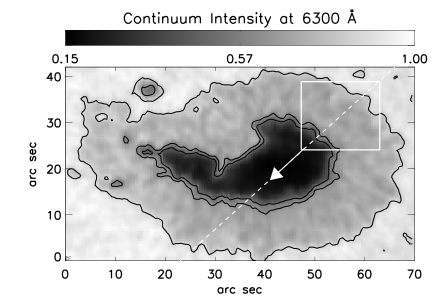
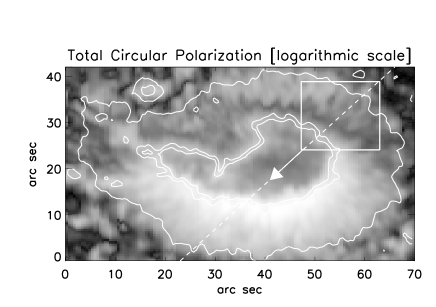
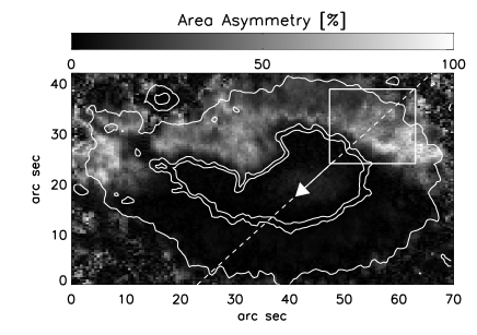
Figure 1: Continuum intensity (top panel), total circular polarization map (middle panel) and area asymmetry maps (bottom panel) of NOAA 8545. The contours correspond to the levels 0.45, 0.6 and 0.85 in units of the quiet sun intensity I_C. The outermost boundary defines the sunspot radius $r=R$. The arrow points towards the direction of the disk center passing through the darkest umbral region (this defines the line of symmetry). The selected region for the inversion is indicated by the white square box on the limbward side of the penumbra, centered on the line of symmetry of the sunspot, where the area asymmetry reaches the largest values.

3 Uncombed model and inversion strategy

Our inversion strategy considers a geometrical model, defined by a set of physical parameters ${\rm{\bf X}}$  (magnetic field vector, temperature, velocity) that enter the Radiative Transfer Equation and are used to produce synthetic Stokes profiles. By comparing the synthetic profiles and the observed ones, the original set of parameters is iterated in some fashion until convergence is achieved. The geometrical model we have selected as representative of the penumbral fine structure is the same as in Paper II, id est: a modification of the uncombed model of Solanki & Montavon (1993). A detailed description of the implementation of the uncombed model into an existing inversion code and its peculiarities can be found in Paper II (Sect. 2). Here we simply discuss its main features for the sake of completeness.

In order to produce synthetic Stokes profiles under the uncombed model, the Radiative Transfer Equation is solved along two different ray paths (see Fig. 2), one of them piercing the flux tube cross section (dashed line) and another passing through the atmosphere that surrounds the flux tube (dot-dashed line). In this simplification the flux tube has a rectangular cross section. The synthetic Stokes vector, $\rm{\bf{S}}_{\rm syn}(\lambda)$, to be compared with the observed ones is obtained according to:

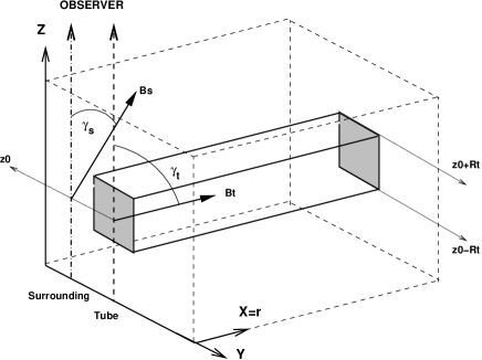
Figure 2: Example of the geometrical scheme used in the inversion. The radiative transfer equation is solved along the 2 rays (dashed and dot-dashed lines) representing the embedded flux tube and surrounding atmosphere, respectively. $\gamma_{\rm s}$ and $\gamma_{\rm t}$ refer to the inclination of the magnetic field vector with respect to the observer. In this picture, for simplicity the heliocentric angle is $\theta=0$ and $\gamma_{\rm t}=90^{\circ}$. The flux tube structure is sampled using one single ray (i.e: our model simplifies the shape of the flux tube into a rectangular cross section).

$$\begin{split}\rm{\bf{S}}_{\rm syn}(\lambda)=&\alpha_{q}\rm{\bf{S}}_{q}(\lambda)\\ &+(1-\alpha_{q})[(1-\alpha_{t})\rm{\bf{S}}_{s}(\lambda)+\alpha_{t}\rm{\bf{S}}_{t}(\lambda)]\end{split}$$ (1)

where the indexes ’s’, ’t’ and ’q’ refer to the surrounding, flux tube and quiet Sun (stray light) contributions respectively. The components of the Stokes vector are the intensity and polarization profiles S$=(I,Q,U,V)$, with S${}_{\rm q}=(I_{q},0,0,0)$ being the intensity profile of the observed spectral lines obtained from the two-component model for the quiet sun from Borrero & Bellot Rubio (2002). $\alpha_{\rm t}$ and $\alpha_{\rm q}$ are the fractional areas of the resolution element occupied by the flux tube and quiet Sun, respectively. If the stratification of the physical parameters in the surrounding atmosphere is denoted as X${}_{\rm s}(z)$ (see dot-dashed line in Fig. 2), then the parameters along the flux tube atmosphere acquire the following form:

$${\rm{\bf X}}_{\rm t}(z)=\left\{\begin{array}[]{ll}{\rm{\bf X}}_{\rm t}&\rm{if}\;\;\;z\in[z_{0}-R_{\rm t},z_{0}+R_{\rm t}]\\ {\rm{\bf X}}_{\rm s}&\rm{otherwise}\end{array}\right.$$ (2)

where, as indicated by Fig. 2, $z_{0}$ is the height where the axis of the flux tube is located and $R_{\rm t}$ is its radius. On the right hand side of Eq. 2, X_t is height independent. Along the surrounding atmosphere X_s is also constant with height, with the exception of the temperature, for all physical parameters. For the temperature stratification T${}_{\rm s}(z)$ we have chosen, as in Paper II, the penumbral model of Del Toro Iniesta et al. (1994). Note that Eq. 2 ensures that the physical stratifications along the flux tube atmosphere (vertical dashed line in Fig. 2) are the same as in the surrounding atmosphere above and beneath the flux tube: $z<z_{o}-R_{\rm t}$ and $z>z_{o}+R_{\rm t}$. At the lower and upper boundaries of the flux tube ($z^{*}=z_{0}\pm R_{\rm t}$) the physical quantities encounter a sharp transition of magnitude $\Delta$X$=$X${}_{\rm t}(z^{*})-$X${}_{\rm s}(z^{*})$. These jumps/gradients are the essential ingredients of this model to explain the net circular polarization (NCP) observed in the sunspot penumbra (Sánchez Almeida & Lites 1992; Solanki & Montavon 1993; cf. Martínez Pillet 2000). Finally, we shall mention that both the surrounding magnetic atmosphere and the flux tube are forced to be in total pressure balance at each height (see Sect. 2 in Paper II for details).

Once the synthetic profiles are computed for an initial guess of free parameters, a merit function is constructed by comparing with the observed penumbral profiles:

$$\chi^{2}=\frac{1}{L}\sum_{j=1}^{4}\sum_{k=1}^{M}[S_{\rm obs}^{j}(\lambda_{k})-S_{\rm syn}^{i}(\lambda_{k})]^{2}w_{j}^{2}$$ (3)

In this equation, $L$ stands for the total number of free parameters in the uncombed model (i.e.:17, see paper II). The index $j=1,...,4$ denotes the four components of the Stokes vector, while $k$ samples each profile in the wavelength direction. Finally, the weighting factor $w_{j}$ is used to favor some spectral lines or polarization states. The weights we have used in our inversions are indicated in Table 2. We are giving special attention to the Stokes $V$ signal for the neutral iron lines at 6301.5 and 6302.5 Å. This is because we are specially interested in extracting the information contained in the net circular polarization (i.e.: gradients along the line of sight in the physical parameters, radius of the penumbral flux tubes, etc.). In addition, some extra weight has been given to the total intensity signal, Stokes $I$, of the Ti I line at 6303.7 Å. The combination of the very small excitation energy of this line and the relatively low ionization energy of Titanium, makes it fairly sensitive to variations in the temperature stratification. In fact, the Ti I line behaves similarly to the OH lines blended with the Fe I 15652.5 Å  line (see Paper II), displaying a high equivalent width in the umbra and at the umbral-penumbral boundary, which rapidly decreases at larger radial distances from the center of the sunspot. The polarization profiles of the last two lines in Table 2 are small compared to those of the first two Fe I lines. Therefore, they are more affected by noise and are of relatively minor importance during the inversion.

Table 2: Relative weights, $w_{j}$, entering in the merit function $\chi^{2}$, for each spectral line and each component of the Stokes vector.

Species	$\lambda_{0}$	$w_{i}$	$w_{q}$	$w_{u}$	$w_{v}$
Fe I	6301.5012	1	1	1	8
Fe I	6302.4916	1	1	1	8
Fe I	6303.4600	1	0.2	0.2	0.2
Ti I	6303.7560	4	0.2	0.2	0.2

Besides the $\chi^{2}$ function from Eq. 3, its derivatives with respect to the free parameters of the problem are computed numerically. A Levenberg-Marquadrt non-linear inversion algorithm is fed with these ingredients in order to iteratively modify the initial guess set of parameters, ${\rm{\bf X}}$₀  (guess magnetic field vector, guess velocity), until a minimum in the merit function is reached. The inversion code described by Frutiger et al. (1999, 2000) and Frutiger (2000) is employed.

4 Inversion results

We have selected for the inversion the region enclosed by the square in Fig. 1. It lies on the limb side of the penumbra, covers an area of about 15$\times$15 arc sec and encloses the line of symmetry of the sunspot. This region was selected because, as can be seen in Fig. 1 (bottom panel), there is a maximum in the area asymmetry of the circular polarization profiles, and hence it seems very suitable to constrain the values for the flux tube radius. The profiles in each spatial pixel are inverted individually starting always from the same set of guess parameters. Let us first give some attention to the quality of the fits produced by the uncombed model. In Fig. 3 we present some examples of the observed and fitted Stokes $V$ profiles for three pixels located at increasing distance from the sunspot center. The fits to the observed data are reasonably accurate, with differences normally well below 0.5%  of the continuum intensity. Even Stokes $V$ profiles with typical shapes of Stokes $Q$ and $U$ (see Sánchez Almeida & Lites 1992), are almost perfectly reproduced (Fig. 3; middle panels), as are single-lobed Stokes $V$ profiles (Fig. 3; bottom panels). Note that, in contrast to the Fe I lines at 1.56 $\mu$m, these fits cannot be achieved by simple 2 component models that neglect gradients along the line of sight in the magnetic field vector and velocity (see Papers I and II). The reason is that the produced area asymmetry with such models would be zero, giving rise to Stokes $V$ profiles that will have equal positive and negative areas (although they may have several lobes due to the cross-over effect) in strong contrast to the observed profiles (see Fig. 3).

Figure 3: Three examples of observed (filled circles) and fitted (solid lines) Stokes $V$ profiles for Fe I 6301.5 (left panels) and Fe I 6302.5 Å  (right panels) lines. These profiles have been taken from three locations with increasing radial distance: $r/R=0.45,0.65,0.85$, such that the upper panel corresponds to the inner penumbra and the bottom panel lies at the outer boundary of the sunspot. The observed and fitted Stokes $V$ area asymmetry, $\delta A$ are also indicated.

As a result of the inversion, the stratifications of the different physical parameters with height in the atmosphere were obtained for both the flux tube component (dashed ray path in Fig. 2) and the surrounding atmosphere (dot-dashed ray path in Fig. 2). We have extracted, for all inverted pixels, the values of the physical parameters (temperature, LOS velocity, magnetic field strength and inclination, gas pressure etc.) at $z=z_{0}$ and plotted them in Fig. 4, as a function of the normalized radial distance in the penumbra $r/R$, with $R$ being the radius of the sunspot as defined by the outermost contour in Fig .1. For all those parameters, except for the temperature, we plot separately the radial behavior along the flux tube (dashed lines and light gray shaded area) and its surrounding atmosphere (dot-dashed line and dark gray shaded area). The dashed and dot-dashed lines indicate the average properties, at a given radial distance, of the flux tubes and surrounding atmosphere, while the shaded areas indicate the maximum deviations from the average values obtained from all inverted points at the same radial distance. For the temperature we plot (solid line) the difference between the flux tubes and the magnetic surrounding atmosphere. The filling factor of the flux tube component, $\alpha_{t}$ (dashed line in Fig. 4; bottom left panel) corresponds, obviously to the flux tube alone, with $1-\alpha_{t}$ being the area covered by the surrounding atmosphere (Eq. 1). In this same plot the amount of stray light contamination $\alpha_{\rm q}$ is represented by the solid line. We retrieve consistent values with those found by Lites et al. (1993) who analyzed ASP data of another sunspot.

As in previous investigations (Borrero et al. 2004, 2005), we have transformed the magnetic field inclination (middle left panel in Fig. 4), that is always obtained in the observer’s reference frame from the inversion, into the local reference frame. Therefore, in the following we discuss the zenith angles $\zeta$ instead of the observer frame inclination $\gamma$, with $\zeta=90^{\circ}$ meaning that the magnetic field is parallel to the solar surface (marked with a horizontal dotted line in the middle left panel of Fig. 4). The lower right panel in Fig. 4 shows the gas pressure along the penumbral flux tubes (dashed line) and surrounding atmosphere (dot-dashed line) at $z=z_{0}$. The gas pressure difference between these two components is indicated by the solid line. As imposed, $\Delta P_{\rm gas}\propto\Delta B^{2}$ since at the same height both atmospheres are in lateral pressure balance (see Eq. 4 in Paper II).

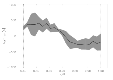
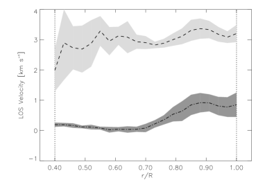
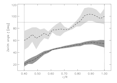
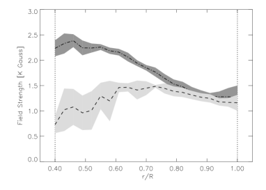
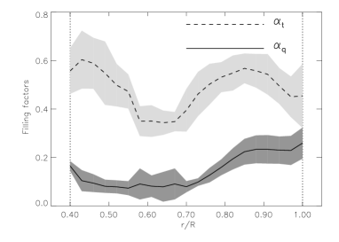
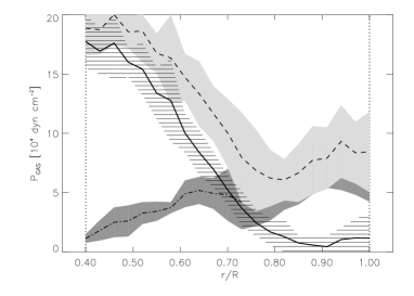
Figure 4: Radial variation of the properties of the magnetic surrounding (dot-dashed lines) and the penumbral flux tube (dashed lines). Shaded areas represent the maximum deviations around the mean obtained from the inversion of all pixels at a given radial distance. From left to right and top to bottom: temperature difference between the flux tube and its surroundings, LOS velocity, magnetic zenith angle $\zeta$, magnetic field strength $B$, flux tube filling factor $\alpha_{t}$ (dashed line) and fraction of stray light $\alpha_{\rm q}$ (solid line), and gas pressure along the flux tubes (dashed), surrounding atmosphere (dot-dashed) and difference between them (solid line and area with horizontal stripes). All quantities have been taken at a geometrical depth that corresponds to the central position of the flux tube: $z=z_{0}$.

4.1 Discussion

A comparison of the results plotted in Fig. 4 with those obtained with the Fe I 1.56 $\mu$m lines by means of the uncombed model (see Paper II; Figs. 5 and 6) shows very similar radial trends. It is gratifying to see that the same model gives so similar results when applied to a set of spectral lines with very different atomic properties and thermodynamic sensitivities. In particular:

• Flux tubes appear hotter than the surrounding atmosphere in the inner penumbra, supporting our previous results from the inversion of the Fe I lines at 1.56 $\mu$m (see Fig. 3; top left panel).

• Flux tubes are inclined with respect to the vector normal to the solar surface in the inner penumbra, $\zeta_{\rm tub}\sim 60^{\circ}$ and become horizontal $\zeta_{\rm tub}\sim 90^{\circ}$ in the middle penumbra (see Fig. 3; middle left panel). At the outer penumbra $r/R>0.8$ for most spatial pixels the flux tubes start to bend down, $\zeta_{\rm tub}>90^{\circ}$, as if returning into the solar interior. Very similar radial dependences were found in Papers I and II.

• The line of sight velocity along the flux tubes (dashed line in Fig. 3; top right panel) is already significant at the inner penumbra $v_{\rm los}\sim 2$ km s^-1. It increases slightly up to $v_{\rm los}\sim 3$ km s^-1 and remains fairly constant for $r/R>0.5$. We do not detect here any abrupt decrease of the flow speed at large radial distances as seen in Paper II. There is also no sign of any enhancement in the flux tube temperature in the outer penumbra. This seems to imply that the signatures of shock fronts due to supercritical speeds reported by Borrero et al. (2005) are not universally seen in sunspot penumbrae. Indeed, the sunspot analyzed in this work is closer to the center of the solar disk than that analyzed in Paper II, and therefore, the LOS velocities obtained here are less representative of the true velocities. Results at smaller radial distances are however, completely consistent with those obtained from the inversion of the Fe I lines at 1.56 $\mu$m. In particular, the high Evershed velocities found in the inner penumbra (Fig. 4, top right panel), suggest that the penumbral flux tubes emerge into the photosphere from subphotospheric layers already carrying high velocities. This agrees with the model results of Schlichemaier et al. (1998a, 1998a, 1999) and Schmidt & Schlichenmaier (2000).

• The magnetic field inclination and line of sight velocities found in the surrounding component are also compatible with (in fact, they are strikingly similar to) those obtained in Papers I and II (see e.g. Fig. 5 and 6 in Borrero et al. 2005).

• The field strength in the surrounding atmosphere rapidly decays radially, while along the flux tube it seems to increase at first until $r/R=0.6$ and slowly decreases afterward. Note however that if these averaged flux tube properties would correspond to a single flux tube that crosses the penumbra, the magnetic field in the inner footpoint, $B\sim 750$ G would be smaller than in the outer footpoint, $B\sim 1100$ G. Such a radially increasing magnetic field is in good agreement with the requirement of the siphon flow mechanism to drive the Evershed flow in an homogeneous penumbra (see Montesinos & Thomas 1997 and references therein). This particular behavior must be considered with some caution however (the Fe I lines at 1.56 $\mu$m did not reveal this behavior in Papers I and II; see also next paragraph). The main result is still consistent with our previous work, that is: while the surrounding magnetic field decreases radially very rapidly, the field strength along the flux tube exhibits a much smaller and slower variation, being $B_{\rm sur}>>B_{\rm tub}$ in the inner penumbra, but $B_{\rm sur}\sim B_{\rm tub}$ at the outer sunspot boundary. Since the radial dependence of the gas pressure difference at $z=z_{0}$ between the flux tubes and their magnetic surroundings scales as $\Delta B^{2}$ this implies, in agreement with Papers I and II, that the gas pressure difference decreases abruptly with radial distance in the penumbra (see Fig. 3; bottom right panel). This gas pressure excess in the flux tubes at the inner penumbra is of course consistent with the higher temperatures found there.

• The individual behaviour of the gas pressure in the penumbral flux tubes and their magnetic surroundings (Fig. 4; bottom right panel) is also instructive. Whereas the gas pressure in the flux tube’s surroundings slowly increases outwards, along the flux tube it displays a rapid drop. In principle, such a pressure gradient as seen in the flux tubes should suffy to drive a siphon flow. However, as already mentioned in Paper II, such a conclussion is correct only if the flux tube is located at the same absolute geometrical height in the inner and the outer penumbra. Since the central position of the flux tube $z_{0}$ may change radially if the Wilson depression were to depend on $r/R$, we cannot conclude that what we see is actually a siphon flow (although the results are completely consistent with one). However, we can the argument around and assume that this is the case. Then we can estimate by how much thee flux tubes have risen from the inner to the outer penumbra: $z_{0}(r/R=1.0)-z_{0}(r/R=0.4)\lesssim 100$ Km. These results are only slightly smaller than those found by Solanki et al. (1993) and Mathew et al. (2004)

• The properties obtained for the flux tube atmosphere are always less accurate that those for the magnetic atmosphere that surrounds them, in particular in the inner penumbra, where the light gray shaded areas indicating the deviations with respect to the average flux tubes properties are largest. This indicates caution when interpreting our results for $r/R<0.5$. The reason for this is to be found in the information contained in the polarization signals near the umbra, where for example, the Stokes $V$ profiles do not show any particular peculiarities (see Fig. 3; top panels) or distinctive signal of the presence of two different components within the resolution element.

4.2 Vertical extension of the Penumbral Flux tubes

Already in Papers I and II, where the umcombed model was applied to the Fe I lines at 15648 and 15652 Å , we pointed out that their visible counterparts (Fe I lines at 6300 Å), being far more sensitive to the vertical stratification in the physical parameters, might help to constraint the values for the vertical extension of the penumbral fibrils. In this section we will investigate this issue.

In order to produce a non vanishing net circular polarization an atmospheric model must include gradients along the line-of-sight in the velocity and magnetic field vector (Landolfi & Landi Degl’Innocenti 1996). In the case of the penumbra of sunspots, the net circular polarization observed in the Fe I lines at 6300 Å  is so large that gradients in the inclination of the magnetic field and line-of-sight velocity as large as $\Delta\gamma\simeq 45^{\circ}$ and $\Delta\rm v_{los}\simeq 1.5$ km s^-1 must be introduced (Sánchez Almeida & Lites 1992).

Such gradients would produce large curvature forces and electric currents that are difficult to match with the idea of a sunspot in hydrostatic equilibrium (Solanki et al. 1993). A way out of this problem was proposed by Solanki & Montavon (1993) who realized that including a three layered atmospheric model where the middle one would have larger velocities and a more horizontal magnetic field could reproduce the observed NCP with no need to invoke net (i.e. large scale) gradients along the line of sight, but rather strong gradients on a small scale that are compensated as the line-of-sight crosses the three atmospheric layers. This is the basic idea of the uncombed model. In our representation of the uncombed model these three layers are identified with the different stratifications along the dashed ray path in Fig. 2. We have already identified the intermediate layer as a horizontal flux tube (carrying the Evershed flow) which is embedded in a magnetic surrounding where the magnetic field is more vertical and essentially at rest. In addition, we are considering a pure surrounding atmosphere (dot-dashed line in Fig. 2; see also Martínez Pillet 2000). Note that since the physical parameters along the surrounding atmosphere are constant with height (see Sect. 3) no net circular polarization is produced here. The NCP is exclusively produced by the ray that crosses the flux tube due to the strong gradients present at the tube’s upper and lower boundaries: $z^{*}=z_{0}\pm R_{\rm t}$.

This realization of the uncombed model has been applied in Paper II to penumbral spectropolarimetric data observed in the Fe I lines at 1.56 $\mu$m. This allowed us to characterize the horizontal inhomogeneities of the penumbral fine structure, but we were not able to model the vertical ones. Since these lines show only small amounts of NCP (with typical values for the area asymmetry of $\delta A\sim 3-5$ %), the positions of the boundary layers where the gradients along the line of sight are produced, therefore the thickness of the penumbral flux tubes, were not properly constrained in the inversion process.

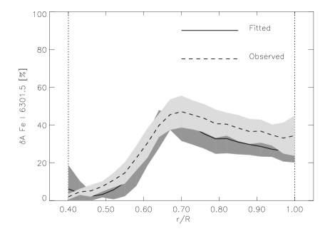
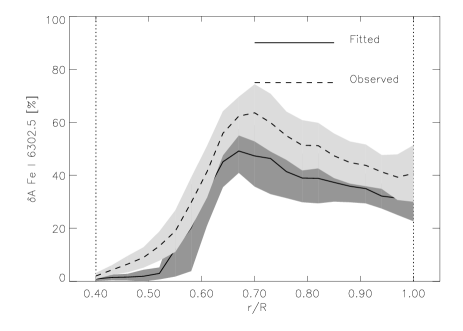
Figure 5: Top panel: Scatter plot of fitted Stokes $V$ area asymmetry versus observed values. The straight line indicates the expectation values. Middle panel: radial variation of the area symmetry of the observed (dashed line) and fitted (solid line) Fe I 6301.5 Å  Stokes $V$ profiles. Shaded areas corresponds to the maximum and minimum deviations from the mean. Bottom panel: same, but for Fe I 6302.5 Å.

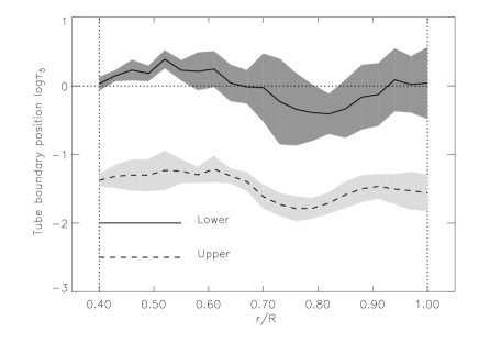
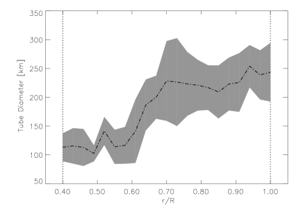
Figure 6: Top panel: locations, in the optical depth scale, of the lower (solid line) and upper (dashed line) boundaries of the flux tube as a function of the radial distance in the penumbra. Bottom panel: inferred flux tube diameter as a function of $r/R$.

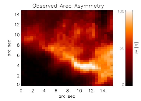
Figure 7: Top panel: Map of the area asymmetry in the white square box in Fig. 1. Top panel: observed area asymmetry. Bottom panel: area asymmetry produced by the uncombed model.

The area asymmetry in the Fe I lines at 6300 Å  is so large that the vertical structure (i.e. discontinuities along the line-of-sight produced at the flux tube boundaries) of the magnetic field and velocity vectors play the leading role. Fig. 5 (top panels) demonstrates that the uncombed model now reproduces the large observed area asymmetry of the visible Fe I lines very well (cf. Fig.  7 in Paper I or top panel of Fig. 7 in Paper II; see also Fig. 18 in Sánchez Almeida 2005). As a function of the radial distance (Fig. 5; middle and bottom panels) we see that the observed area asymmetry (dashed lines) increases radially up to $\delta A\sim 50-70$ % in the middle penumbra ($r/R\sim 0.7$) and decreases slowly hereafter. The area asymmetry of the fitted profiles (solid lines) mimics this behavior, although it slightly underestimates the observed values.

Note that the radial behavior of both the observed and the fitted NCP follow the prediction of Solanki & Montavon (1993) in their Fig. 4. They realized than even though the amount of NCP generated at the flux tube’s boundaries depends on the magnitude of the jump in the velocity and magnetic field inclination at that location, the NCP displayed a maximum where the average line of sight magnetic field between the flux tubes and their magnetic surroundings, $\tilde{\gamma}=\frac{1}{2}[\gamma_{\rm tub}+\gamma_{\rm sur}]$, was close to 90^∘ (i.e.: in the neutral line of the sunspot; see black region in the limb side penumbra of the middle panel of Fig. 1). This is exactly what happens in our case. In Fig. 4 one can see that although $\Delta v_{\rm los}\sim 3$ km s^-1 and $\Delta\zeta\sim 40^{\circ}$ at all radial distances, the amount of NCP produced (middle and bottom panels in Fig. 5) varies with radial distance, reaching its maximum where $\tilde{\gamma}=90-100^{\circ}$.

In addition to the average magnetic field inclination, the position of the upper and lower boundaries of the flux tube $z^{*}=z_{0}\pm R_{\rm t}$ play also a significant role in producing NCP as we show below. Fig. 6 (upper panel) presents the position (in the $\log\tau_{5}$ scale) of the upper (dashed) and lower (solid) flux tube boundaries as a function of the radial distance in the penumbra. The horizontal line at $\log\tau_{5}=0$ has been plotted in order to indicate when discontinuities along the line of sight start producing a significant amount of NCP in the Fe I lines at 6300 Å  (when $\tau_{5}\leq 1$; see Fig. 8b in Paper I). Our Fig. 6 shows that in the inner penumbra, the lower boundary of the flux tube lies right beneath the continuum level, and therefore does not contribute significantly to the generation of NCP. The area asymmetry observed at small radial distances (see Fig. 5; middle and bottom panels) is of the order of $\delta A\sim 0-20$ % and is mainly due to the upper flux tube boundary. At $r/R>0.6$ the lower flux tube boundary moves above the $\log\tau_{5}=0$ level and therefore starts contributing, together with the upper boundary, to the generation of area asymmetry. Note that it is at these radial distances that the observed $\delta A$ values are largest.

The bottom panel in Fig. 6 shows the radial variation of the penumbral flux tube diameter as inferred from the uncombed model. According to our results the vertical extension of the penumbral flux tubes is roughly 100-300 km, in good agreement with previous investigations based only on net circular polarization considerations (Solanki & Montavon 1993; Martínez Pillet 2000,2001). It is also comparable to the horizontal width of the penumbral fibrils observed in the continuum images at very high spatial resolution by Sütterlin (2001), Scharmer et al. (2002) and Sütterlin et al. (2004). Note that, although the penumbral flux tubes are thinner in the inner penumbra on a geometrical scale, the thickness is almost constant with radial distance in the optical depth scale. This opacity excess is explained by the enhanced gas pressure and temperature inside the penumbral flux tubes at the inner penumbra. Note that the vertical width of the flux tube is an upper limit in the sense that a broader and tube would have difficulty to reproduce the observations. The same is true to a narrower tube, if only a single tube lies along the line of sight. However, we cannot rule out that multiple flux tubes lying on top of each other cannot reproduce the observations.

Finally, in Fig. 7 we present a close up of the square region in Fig. 1 (middle panel) that has been analyzed in this work. The color code indicates the observed area asymmetry (top panel) and the area asymmetry produced by the uncombed model (bottom panel). The similarity is striking, with the uncombed model being able to reproduce much (but not all) of the small scale behavior of the NCP.

4.3 Magnetic flux conservation

As we have demonstrated the uncombed model is able to reproduce with good accuracy the area asymmetry in the circular polarization profiles using flux tubes of some 100-300 km in diameter. In this section we check whether the model also satisfies the condition ${\bf\nabla}\cdot{\bf B}=0$. Let us consider cylindrical coordinates where the vectors ${\bf e_{\rho}}$ and ${\bf e_{\phi}}$ are contained in the plane perpendicular to the flux tube’s axis ($\bar{YZ}$ plane in Fig. 2) and the vector ${\bf e_{x}}$ points along the tube’s axis (i.e: radial direction along the penumbra). The null divergence condition is written as:

$${\bf\nabla}\cdot{\bf B}=\frac{1}{\rho}\frac{\partial}{\partial\rho}\left(\rho B_{\rho}\right)+\frac{1}{\rho}\frac{\partial B_{\phi}}{\partial\phi}+\frac{\partial B_{x}}{\partial x}=0$$ (4)

This condition must be satisfied locally by both the flux tube and the surrounding atmosphere. Let us first focus on the surrounding magnetic field ${\bf B_{\rm s}}$. The third term in Eq. 4 (derivative along the tube’s axis) can be written as:

$$\frac{\partial B_{xs}}{\partial x}=\frac{\partial B_{rs}}{\partial r}=\frac{\partial}{\partial r}[B_{\rm s}(r)\sin\zeta_{\rm s}(r)]$$ (5)

where we considered that the $x$ coordinate (tube’s axis) points radially in the penumbra. This in turn means that we can use the the radial dependences of $B_{\rm s}$ and $\zeta_{\rm s}$ (zenith angle) from Fig. 4. It is clear that, the surrounding magnetic field has to bend aside in order to accommodate the flux tube. This means that none of the first two terms in Eq. 4 will be individually identical to zero. Under our model assumptions, these two derivatives can not be computed. Nevertheless, assuming that the null divergence condition is satisfied, we can calculate:

$$-\frac{1}{\rho}\frac{\partial}{\partial\rho}\left(\rho B_{\rho s}\right)-\frac{1}{\rho}\frac{\partial B_{\phi s}}{\partial\phi}=\frac{\partial}{\partial r}[B_{\rm s}(r)\sin\zeta_{\rm s}(r)]$$ (6)

As far as the flux tube’s magnetic field ${\bf B_{\rm t}}$ is concerned, the magnetic field in our model is parallel to the tube’s axis and therefore $B_{\rho}$ and $B_{\phi}$ in Eq. 4 are identically zero. Interestingly, a study of the magnetic configurations leading to a magnetohydrostatic solution (Borrero 2004; Borrero et al. 2006, in preparation) shows that the flux tube’s magnetic field must have a non vanishing component in the $\bar{YZ}$ plane. Since our model also samples the flux tube using one ray path only, the first two terms in Eq. 4 can not be computed. Once more, assuming that the null divergence condition is satisfied, we can write:

$$-\frac{1}{\rho}\frac{\partial}{\partial\rho}\left(\rho B_{\rho t}\right)-\frac{1}{\rho}\frac{\partial B_{\phi t}}{\partial\phi}=\frac{\partial}{\partial r}[B_{\rm t}(r)\sin\zeta_{\rm t}(r)]$$ (7)

where the right hand term can be deduced from the observations. We have plotted in Fig. 8 the right hand terms of Eq. 6 and Eq. 7. This allows us to offer an upper limit on the derivatives along the $\bar{YZ}$ plane. It turns out that both the flux tube and surrounding magnetic field are neraly divergence free in the plane perpendicular to the tube’s axis.

$$\frac{1}{\rho}\frac{\partial}{\partial\rho}\left(\rho B_{\rho}\right)+\frac{1}{\rho}\frac{\partial B_{\phi}}{\partial\phi}<0.5\;\;\;{\rm Gauss\;km^{-1}}$$ (8)

Figure 8: $\frac{\partial}{\partial r}[B(r)\sin\zeta(r)]$ as a function of the radial distance in the penumbra, for the external magnetic field (dot-dashed line) and the flux tube magnetic field (dashed line).

5 Conclusions

The uncombed model is able to reproduce satisfactorily the polarization signals emerging from the sunspot penumbra both for the Fe I lines at 6300 Å  and at 1.56 $\mu$m. The area asymmetry in the circular polarization profiles, Stokes $V$, as well as its behavior with radial distance in the penumbra are also reproduced. The azimuthal variation of the NCP observed in both sets of spectral lines also finds a satisfactory explanation in terms of the uncombed model (see Müller et al. 2002; Schlichenmaier et al. 2002).

We stress the important similarities of the results obtained in this work with the results from Papers I and II (compare with our Fig. 3 with Fig. 4 in Paper I and Fig. 5 and 6 in Paper II). This is in spite of the fact that we have inverted different spectral lines (Fe I and OH lines at 1.56 $\mu$m vs. Fe I & Ti I lines at 630 nm). In addition, in our series of papers we have thoroughly studied three different sunspots at three different heliocentric angles, observed with two different telescopes. The remarkable consistency of the results provides strong support for the uncombed model.

It also shows that the results obtained from the inversion of Stokes profiles are entirely consistent if interpreted in the context of this model (contrary to the claim of Spruit & Scharmer 2005). Indeed, the ability to reproduce in detail a variety of spectropolarimetric data must be the hallmark of any successful model of the penumbral fine structure.

Yet, some differences remain between the results obtained from the Fe I 1.56 $\mu$m and Fe I 6300 Å  lines (see e.g.: the radial variation of the flux tube filling factor in Fig. 4; cf. Fig. 5 in Paper II). Recent developments in the existing instrumentation (see Socas-Navarro et al. 2005; Bellot Rubio & Beck 2005) now allow both spectral windows to be recorded simultaneously. It is planned to analyze such observations in order to resolve these discrepancies. Such observations, if made at high resolution, could allow for a simultaneous and accurate determination of the vertical and horizontal structure of the sunspot penumbra.

It is important to note that the inferred vertical sizes for the penumbral flux tubes (around 100-300 km) have been obtained from the interpretation of the polarized spectrum, and in particular, of the net circular polarization, within the assumptions on the geometry of the penumbral fine structure included in the uncombed field model. Although we can not rule out other models, that offering a consistent explanation of the observed profiles, consider flux tubes with smaller sizes, we are confident on the feasibility of the uncombed model since it retrieves vertical extensions for the penumbral fibrils of the same order of the horizontal widths observed by Scharmer et al. (2002) and Sütterlin et al. (2004) from continuum images at high spatial resolution.

Flux tubes as thick as those retrieved here would imply that simulations of penumbral flux tubes embedded in the penumbra (e.g Montesinos & Thomas 1997, Schlichenmaier et al. 1998a,1998b) would need to be revisited, since they all rely on the thin flux tube approximation and therefore they neglect any variation in the physical quantities in the plane perpendicular to the tube’s axis. This will be the subject of a future investigation: Borrero et al. (in preparation).

Last but not least we acknowledge that any model of the sunspot penumbra based on horizontal flux tubes embedded in a magnetic surrounding atmosphere, has indeed a loose thread. As already pointed out by Schlichenmaier & Solanki (2003) such models face serious difficulties to explain the energy transport responsible for the penumbral brightness.

- (1) Barklem, P.S., O’Mara, B.J., 1997, MNRAS, 290, 102
- (2) Barklem, P.S., O’Mara J.O., & Ross, J.E. 1998, MNRAS, 296, 1057
- (3) Bellot Rubio, L.R., Balthasar, H., Collados, M. & Schlichenmaier, R. 2003, A&A, 403, L47
- (4) Bellot Rubio, L.R., Balthasar, H. & Collados, M. 2004, A&A, 427, 319
- (5) Bellot Rubio, L.R., Langhans, K. & Schlichenmaier, R. 2005 A&A, in press
- (6) Bellot Rubio, L.R. & Beck, C. 2005, ApJ, 626, L125
- (7) Borrero, J.M. & Bellot Rubio, L.R., 2002, A&A, 385, 1056
- (8) Borrero, J.M., Bellot Rubio, L.R., Barklem, P.S. & del Toro Iniesta, J.C., 2003, A&A, 404, 749
- (9) Borrero, J.M., Solanki, S.K., Bellot Rubio, L.R., Lagg, A. & Mathew, S.K. 2004, A&A, 422, 1093, Paper I
- (10) Borrero, J.M., PhD thesis (2004). University of Göttingen (Germany), published by Copernicus GmbH ISBN 3-936596-33-0
- (11) Borrero, J.M., Lagg, A., Solanki, S.K. & Collados, M. 2005, A&A, 436, 333, Paper II
- (12) Del Toro Iniesta, J.C., Tarbell, T.D., & Ruiz Cobo, B. 1994, ApJ, 436, 400
- (13) Elmore, D. F. et al. 1992, Proc. SPIE, 1746, 22
- (14) Frutiger, C., Solanki, S.K., Fligge, M. & Bruls, J.H.M.J. 1999 in Solar Polarization workshop, eds. K.N. Nagendra and J.O. Stenflo (Astrophysiscs and Space Science library vol 243), 281
- (15) Frutiger, C., 2000, PhD Thesis, Institute of Astronomy, ETH, Zürich, No. 13896
- (16) Frutiger, C., Solanki, S.K., Fligge, M. & Bruls, J.H.M.J. 2000, A&A, 358, 1109
- (17) Landolfi, M. & Landi degl’Innocenti, E., 1996, SoPh., 164, 191
- (18) Langhans, K., Scharmer, G.B., Kiselman, D., Löfdahl, M.G. & Berger, T. 2005, A&A, 436 1087
- (19) Lites, B.W., Elmore, D.F., Seagraves, P. & Skumanich, A.P. 1993, ApJ, 418, 928
- (20) Martínez Pillet, V. 2000, A&A, 361, 734
- (21) Martínez Pillet, V. 2001, A&A, 369, 644
- (22) Mathew, S., Lagg, A., Solanki, S.K., et al. 2003, A&A, 403, 695
- (23) Mathew, S., Solanki, S.K., Lagg, A., et al. 2004, A&A, 422, 693
- (24) Montesinos, B. & Thomas, J., 1997, Nature, 390, 485
- (25) Müller, D.A.N., Schlichenmaier, R., Steiner, O. & Stix, M., 2002, A&A, 393, 305
- (26) Rouppe van der Voort, L., Löfdahl, M.G., Kiselman, D. & Scharmer, G.B., 2004, A&A, 414, 717
- (27) Sánchez Almeida, J. & Lites, B.W., 1992, ApJ, 398, 359
- (28) Sánchez Almeida, J. 2005, ApJ, 622, 1292
- (29) Scharmer, G., Gudiksen , B.V., Kiselman, D., et al. 2002, Nature, 420, 151
- (30) Schlichenmaier, R., Jahn, K. & Schmidt, H.U., 1998a, A&A, 337, 897
- (31) Schlichenmaier, R., Jahn, K. & Schmidt, H.U., 1998b, ApJ, 483, L121
- (32) Schlichenmaier, R., Bruls, J., & Schüssler, M. 1999, A&A, 349, 961
- (33) Schlichenmaier, R., Müller, D.A.N., Steiner, O. & Stix, M., 2002, A&A, 381, L77
- (34) Schlichenmaier, R. & Solanki, S.K. 2003, A&A, 411, 257
- (35) Schmidt, W. & Schlichenmaier, R., 2000, A&A, 364, 829
- (36) Skumanich, A., Lites, B., Martínez Pillet, V., Seagraves, P. 1997, ApJS, 110, 357
- (37) Socas-Navarro, H., Elmore, D., Pietarila, A., Darnell, T., Lites, B. & Tomczyck, S. 2005, SolPhys, in press
- (38) Solanki, S.K., & Montavon, C.A.P. 1993, A&A, 275, 283
- (39) Solanki, S.K., Walther, U., & Linvingston, W. 1993, A&A, 277, 639
- (40) Spruit, H.C. & Scahrmer, G.B. 2005, A&A, in press
- (41) Sütterlin, P., 2001, A&A, 374, L21
- (42) Sütterlin, P., Bellot Rubio, L.R. & Schlichenmaier, R., 2004, A&A, 424, 1049
- (43) Westendorp Plaza, C., del Toro Iniesta, J.C., Ruiz Cobo, B. et al. 1997, Nature, 389, 47
- (44) Westendorp Plaza, C., del Toro Iniesta, J.C., Ruiz Cobo, B. & Martínez Pillet, V. 2001a, ApJ, 547, 1148
- (45) Westendorp Plaza, C., del Toro Iniesta, J.C., Ruiz Cobo, B. et al. 2001b, ApJ, 547, 1130