Emission lines from rotating proto-stellar jets with variable velocity profiles

Using the Yguazú-a three-dimensional hydrodynamic code, we have computed a set of numerical simulations of heavy, supersonic, radiatively cooling jets including variabilities in both the ejection direction (precession) and the jet velocity (intermittence). In order to investigate the effects of jet rotation on the shape of the line profiles, we also introduce an initial toroidal rotation velocity profile, in agreement with some recent observational evidence found in jets from T Tauri stars which seems to support the presence of a rotation velocity pattern inside the jet beam, near the jet production region. Since the Yguazú-a code includes an atomic/ionic network, we are able to compute the emission coefficients for several emission lines, and we generate line profiles for the H$\alpha$, [O I]$\lambda$6300, [S II]$\lambda$6716 and [N II]$\lambda$6548 lines. Using initial parameters that are suitable for the DG Tau microjet, we show that the computed radial velocity shift for the medium-velocity component of the line profile as a function of distance from the jet axis is strikingly similar for rotating and non-rotating jet models. These findings lead us to put forward some caveats on the interpretation of the observed radial velocity distribution from a few outflows from young stellar objects, and we claim that these data should not be directly used as a doubtless confirmation of the magnetocentrifugal wind acceleration models.

1 Introduction

It is now widely accepted that Herbig-Haro jets are a common by-product of the formation of a low mass star. Initially, it was proposed that these jets originate as stellar winds (Cantó (1980); Hartmann et al. (1982)). However, the apparent correlation between ejection and accretion signatures favoured disk wind models. Blandford & Payne (bland82 (1982)) proposed a model in which a wind is launched from the disk surface through open magnetic field lines which make an angle greater than $30^{\circ}$ with the vertical direction. This was called the magneto-centrifugal model because the centrifugal force exerted in a particle attached to an open magnetic field line (satisfying the condition mentioned above) accelerates it to speeds above the escape velocity. More recently, Ferreira (ferreira97 (1997)) and Casse & Ferreira (2000a ; 2000b ) proposed self-similar jet launching mechanisms arising from an extended region of the accretion disk in which the magnetic field lines have their origin in the disk itself. They analyzed cold and warm models. These models are ruled by three dimensionless parameters: the disk aspect ratio $\varepsilon=h/r$, where $h$ is the disk scale height at the cylindrical radius $r$, the turbulence level $\alpha_{m}=\nu_{m}/V_{A}h$ (where $\nu_{m}$ is the turbulent magnetic diffusivity and $V_{A}$ is the Alfvén velocity at the disk midplane), and the ejection index $\xi=$ d ln $\dot{M}_{a}$ / d ln $r$ (where $\dot{M}_{a}$ is the accretion rate), which gives the efficiency of the launching process. In the cold models, the enthalpy at the jet basis is null, while the warm jet launching models have some heating source that provides additional thermal energy. The ejection efficiency for cold jets is at most $\xi\sim 0.01$ while warm jets could have efficiencies of up to $\xi\sim 0.5$. Another kind of disk model is the so called X-wind (Shu et al. shu..94 (1994)). In this case, the disk is truncated exactly at the corotation point and the jet is launched from this truncation radius. In both models, the rotation of the disk plays a very important role. The exact point or region from which the jet arises is still under debate.

Although the magneto-centrifugal acceleration (hereafter, MCA) is widely accepted as being the general mechanism behind the launching of a disk wind, the lack of observational support for it until recently has contributed to keep the subject open. In the last few years, however, observations of a few jets associated with young T Tauri stars appear to support this model, since the interpretation of the radial velocity profiles close to the launching region is both qualitatively and quantitatively in agreement with them (e.g., Bacciotti et al. bacci02 (2002); Coffey et al. coffey04 (2004); Woitas et al. woitas05 (2005)). These authors claim that, for a few jets associated with T Tauri stars (namely DG Tau, Th28, RW Aur and LkH$\alpha$321), there is a trend in the radial velocity pattern which indicates that the jet is rotating. Furthermore, they find that the rotation velocity implied by the observed radial velocity distribution is in good agreement with the rotational profile expected for a wind launched by the MCA model (see Pesenti et al. pesenti (2004)).

Bacciotti et al. (bacci02 (2002)) have carried out HST/STIS measurements of the [O I]$\lambda\lambda$6300,6363 and [S II]$\lambda\lambda$6716,6731 emission line profiles of the DG Tau jet. The observation was designed to construct a datacube, changing the position of the long slit (of $0\aas@@fstack{\prime\prime}1\times 52\aas@@fstack{\prime\prime}$) several times. The datacube was then used to determine the spatial distribution of the radial velocity. In particular, they have taken spectra for seven different positions perpendicular to the DG Tau jet, for a given distance from the source, by offsetting each slit position by $0\aas@@fstack{\prime\prime}07$. Assuming that the jet is axisymmetric, they carefully determine the position of the jet axis, by determining the peak of each emission line, and radial velocities associated with symmetrically disposed positions (on both sides of the jet axis) were measured. The line profiles obtained by Bacciotti et al. (bacci02 (2002)) were decomposed into two components, and the medium-velocity component (hereafter, MVC) was used to perform the analysis. The radial velocity (associated with the MVC) was then plotted against the slit position (i.e., distance from the jet axis), for four regions of increasing distance from the source (named regions I, II, III and IV, at distances from the source of $0\aas@@fstack{\prime\prime}075$, $0\aas@@fstack{\prime\prime}175$, $0\aas@@fstack{\prime\prime}275$ and $0\aas@@fstack{\prime\prime}4$, respectively). They found that the radial velocity shift for positions symmetrically distant from the jet axis is systematically negative, regardless of the chosen region (I, II, III or IV) or the emission line. This systematic negative shift in the radial velocity differences was interpreted by the authors as evidence that the jet is rotating.

The values found for the rotational velocity of the DG Tau jet, in the range of 6-15 km s^-1, are in agreement with the values predicted by the MCA models, for an assumed $\dot{M}_{jet}/\dot{M}_{acc}\sim 0.1$ (which is a bona fide value for these young stellar systems and, in particular, for the DG Tau system). This result, if combined with the fact that the circunstelar disk that surrounds DG Tau shows a velocity pattern [extracted from the ¹³CO(2-1) data by Testi et al. testi (2002)] that is consistent with a disk rotating in the same direction as the jet, reinforces the MCA scenario. Applying a technique very similar to that of Bacciotti et al. (bacci02 (2002)), Woitas et al. (woitas05 (2005)) have re-analyzed the data from their HST/STIS observations of the RW Aur bipolar flow (see Woitas et al. woitas02 (2002)), and they found the same trend in the radial velocity shifts.

Coffey et al. (coffey04 (2004)), also using the HST/STIS spectrograph, found that the bipolar jets from the T Tauri stars TH28 and RW Aur (see also Woitas et al. woitas05 (2005) for the latter source), as well as the blue-shifted jet from LkH$\alpha$321 also show systematic velocity asymmetries which are consistent with the results obtained by Bacciotti et al. (bacci02 (2002)) for DG Tau. In other words, they also interpret the radial negative (or positive) velocity shifts as a signature of rotation (clockwise or counter-clockwise, depending on the sign of the radial velocity shift; see Coffey et al. coffey04 (2004) for details). In particular, they found that in the TH28 and RW Aur flows, which are bipolar, both the jet and the counter-jet appear to rotate in the same direction, and they use this fact as an argument in favour of the MCA models.

These observational data and, more importantly, their interpretation as a jet rotation signature, lead some authors to use them to constrain the wind launching region on the surface of the accretion disk. Pesenti et al. (pesenti (2004)) used their self-similar MHD disk wind solutions to investigate the possible influence of projection or excitation gradients in the relation between the rotation signature and the true azimuthal velocity profile. They computed cold and warm models with different parameters and found that warm models, with an outer radius $\sim$ 3 AU, better reproduce the observations of DG Tau. They found that both cold and warm disk solutions predicts increasing values for the radial velocity shifts for increasing distances from the jet axis. However, the values predicted for the velocity shifts in the warm solution are systematically smaller than those predicted by the cold disk solutions, in better agreement with the observations. They also argue that the shift in the radial velocity for the computed models are systematically smaller than the values given by the true rotational profiles, and that this effect is more pronounced near the jet axis.

In a somewhat different approach, Cerqueira & de Gouveia Dal Pino (cerq04 (2004)) have performed three-dimensional SPH numerical simulations of rotating jets. They were able to reproduce the trend in the shift of the radial velocities observed in DG Tau by Bacciotti et al. (bacci02 (2002)), with a model of a precessing (half-opening angle of $5^{\circ}$), variable velocity (300 $\pm$ 100 km s^-1, sinusoidal velocity variation with a $\tau_{pul}=8$ years period) jet. Cerqueira & de Gouveia Dal Pino (cerq04 (2004)) have not computed the emission line profiles, that would allow a direct comparison between the numerical models and the observed data. These authors claim that a magnetic field of intensity of the order of $\approx 1$ $\mu$G is necessary in order to maintain jet stability against lateral expansion due to centrifugal forces. Actually, very recent modeling of observational data carried out by Woitas et al. (woitas05 (2005)) for both lobes of the bipolar outflow from RW Aur also suggest a magnetic collimation mechanism for the jet.

These observations and models are increasingly providing support for a scenario in which the MCA model matches the available observational data (considering the errors estimated from both). However, apart from the very low number of observed sources with this kind of radial velocity pattern (four until now), there are still a few points that should be carefully verified before excluding alternative views, which can also explain the observed data. For example, Soker (soker (2005)) proposed that the interaction between the jet with a warped accretion disk can explain the asymmetry in the radial velocity distribution across the jet beam, although his model is in need of direct observational support (since an inclination between the jet and the outer parts of the accretion disk is assumed).

In this paper, we present the results of a set of fully three-dimensional numerical simulations of a non-magnetic jet that is allowed to precess and rotate. This, together with an ejection velocity time-variability (which produces multiple internal working surfaces), represents a complete scenario for the Herbig-Haro jets, which are believed to present the observational signature of rotation. With a proper calculation of the emission coefficients, the cooling of the gas, and the evolution of the atomic/ionic species, we are able to produce velocity channel maps, and then reconstruct the line profiles for several of the observed forbidden and permitted (namely H$\alpha$) emission lines. We then make a comparison between the radial velocities extracted from these computed line profiles and those from previously published data of HH jets.

The paper is organized as follows. In §2, we describe the numerical technique and the physical parameters of the simulations. The results are presented in §3, and in §4 we discuss these results and their relation with the available observational data.

2 The numerical method and the simulated models

2.1 The Yguazú-a code

The 3-D numerical simulations have been carried out with the Yguazú-a adaptive grid code (which is described in detail by Raga et al. raga00 (2000) and Raga et al. raga02 (2002)), using a 5-level binary adaptive grid. The Yguazú-a code integrates the gas-dynamic equations (employing the “flux vector splitting” scheme of van Leer van (1982)) together with a system of rate equations for the atomic/ionic species: HI, HII, HeI, HeII, HeIII, CII, CIII, CIV, NI, NII, NIII, OI, OII, OIII, OIV, SII and SIII. With these rate equations, a non-equilibrium cooling function is computed. The reaction and cooling rates are described in detail by Raga et al. (raga02 (2002)).

This code has been extensively employed for simulating several astrophysical scenarios such as jets (Masciadri et al. mas (2002); Velázquez, Riera & Raga vela1 (2004); Raga et al. raga04 (2004); Raga et al. raga02 (2002)), interacting winds (González et al 2004a ; 2004b ; Raga et al. 2001a ) and supernova remnants (Velázquez et vel04 (2004); Velázquez et al. 2001a ). It was also tested with laser generated plasma laboratory experiments (Raga et al. 2001b ; Sobral et al. sobral (2000); Velázquez et al. 2001b ).

The computational domain has dimensions of $1.1\times 10^{16}$ cm along the $x-$ and $y-$axes, and of $4.4\times 10^{16}$ cm along the $z-$axis. The grid has a maximum resolution of $8.59\times 10^{13}$ cm along the three axes. Assuming a distance of 140 pc (e.g., Kenyon, Dobrzycka, & Hartmann (1994)), this maximum resolution corresponds to an angular size of $\approx 0\aas@@fstack{\prime\prime}04$.

2.2 The models

Table 1: The simulated models.

$$\begin{array}[]{p{0.2\linewidth}cccc}\hline\cr Model&\tau_{pul.}&\tau_{pre.}&\theta&{\rm rotation?}\\ \hline\cr M1&8&-&-&{\rm no}\\ M2&8&8&5&{\rm no}\\ M3&8&-&-&{\rm yes}\\ M4&8&8&5&{\rm yes}\\ \hline\cr\end{array}$$

The parameters were chosen in order to model the observations of the DG Tau jet. All the simulated models have a time-dependent ejection velocity given by (Raga et al. 2001c ):

$$v_{j}=v_{0}\left[1+A\leavevmode\nobreak\ {\rm sin}\left(\frac{2\pi}{\tau_{pul}}t\right)\right],$$ (1)

where $v_{0}=300$ km s^-1, and $A=0.33$ (giving a jet velocity variability in the range of 200-400 km s^-1) and $\tau_{pul}=8$ years. These parameters are appropriate for producing the velocity structure of the DG Tau microjet (Bacciotti et al. bacci02 (2002); Raga et al. 2001c ; Pyo et al. pyo (2003)). There is also evidence that the DG Tau microjet precesses, with a precessing angle of $\approx 5^{\circ}$ and a precessing period of $\approx 8$ years (e.g.; Lavalley-Fouquet et al. lava2 (2000); Dougados et al. dou00 (2000)). In Table 1 we give the model label (first column), the period (in years) for the velocity variability and for the precession of the jet axis (second and third column, respectively), the half-opening angle of the precession cone (fourth column) and, finally, the presence (or not) of rotation in a given model, expressed by a toroidal velocity profile (see below). The physical parameters of the models presented in Table 1 are, thus, suitable for the study of the DG Tau jet. Finally, we choose an initial number density for the jet $n_{j}=1000$ cm^-3 (with $\eta=n_{j}/n_{e}=10$, where $n_{e}$ is the initial number density for the environment), and a temperature $T_{j}=10^{4}$ K (with $\kappa=T_{j}/T_{e}=10$). We also assume that the initial jet H ionization fraction is of 10%.

In order to investigate the signatures of rotation on the line profiles, we have simulated models with and without an initially imposed toroidal velocity profile (see Table 1). The adopted toroidal velocity is the same as in Cerqueira & de Gouveia Dal Pino (cerq04 (2004)):

$$v_{\phi}=8{\rm km\leavevmode\nobreak\ s}^{-1}\cdot\frac{R_{j}}{R},$$ (2)

where $v_{\phi}$ is the toroidal velocity in km s^-1, $R_{j}$ is the jet radius ($5.6\times 10^{14}$ cm in physical units) and $R$ is the cylindrical radius. We note that this profile has been truncated at a radial distance $=0.15R_{j}$, where the toroidal velocity attains a constant value of $v_{\phi}\simeq 55$ km s^-1.

We should note that the radial dependence of the toroidal velocity depends on the details of the MCA wind model that is considered. For example, the model of Pesenti et al. (2004) predicts a $v_{\phi}\propto R^{-1/2}$ law. In the present paper, we restrict ourselves to the toroidal velocity law given by equation (2), and do not explore other possibilities.

From the temperature, and atomic/ionic/electronic number densities computed in the numerical time-integration, we calculate the emission line coefficients of a set of permitted and forbidden emission lines. We compute the Balmer H$\alpha$ line considering the contributions from the recombination cascade and from $n=1\to 3$ collisional excitations. The forbidden lines are all computed by solving 5-level atom problems, using the parameters of Mendoza (mendoza (1983)).

3 Results

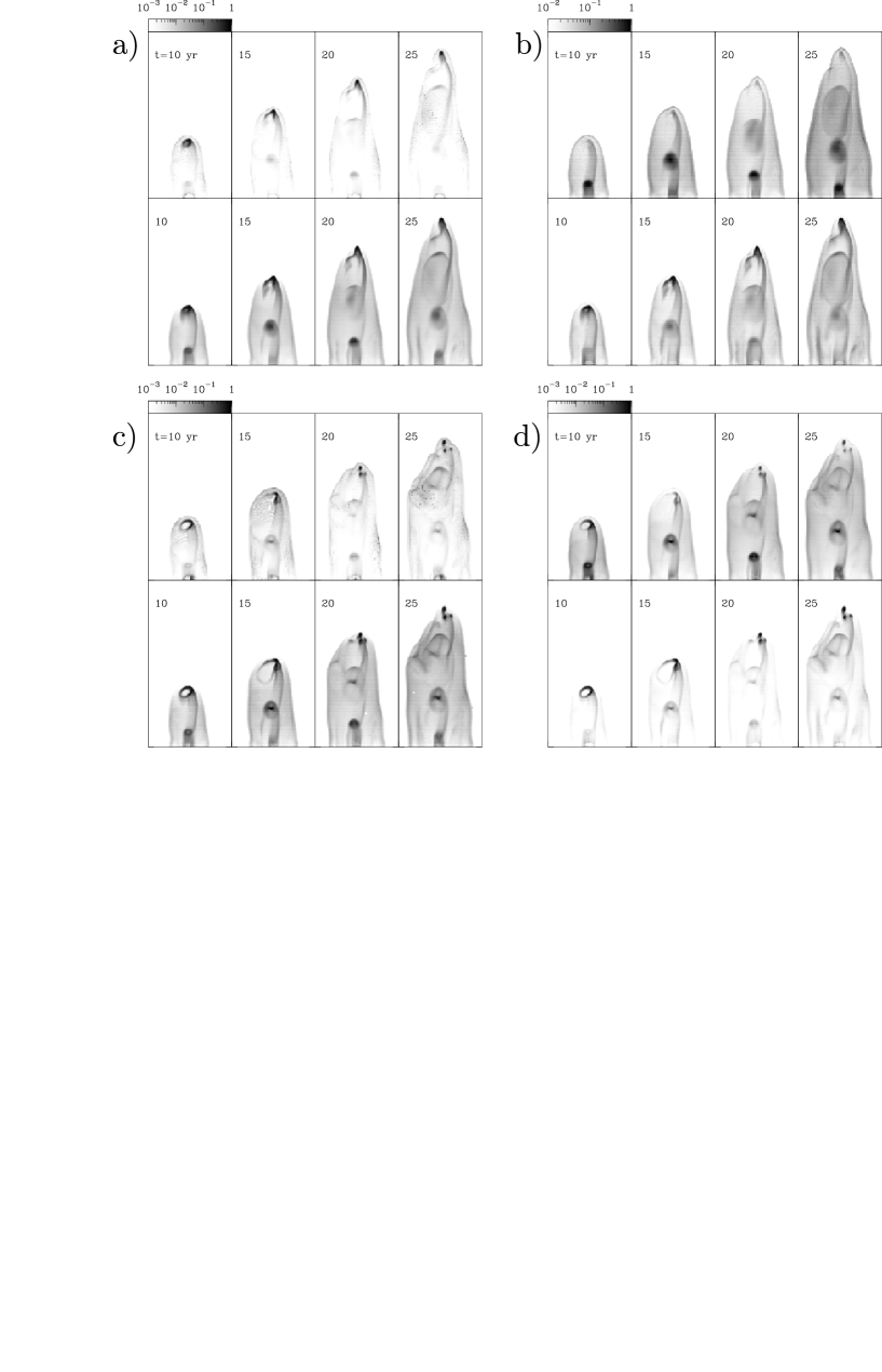
Figure 1: a) Temporal evolution ($t=10$, 15, 20 and 25 years, from left to right) of the emission maps for the H$\alpha$ (top) and [S II]$\lambda$6716 (bottom) lines, computed for model M2 (see Table 1). b) The same as in $a)$ for the [O I]$\lambda$6300 (top) and [N II]$\lambda$6548 (bottom) lines. c) Temporal evolution ($t=10$, 15, 20 and 25 years, from left to right) of the emission maps for the H$\alpha$ (top) and [S II]$\lambda$6716 (bottom) lines, computed for model M4 (see Table 1). d) The same as in $c)$ for the [O I]$\lambda$6300 (top) and [N II]$\lambda$6548 (bottom) lines. The jet in each map was assumed to have an angle with respect to the line of sight of $45^{\circ}$. The bars on top of each diagram give the normalized flux. [See the electronic edition of Astronomy & Astrophysics for a color version of this figure.]

Figure 1 shows the temporal evolution for the emission maps of models M2 (Fig 1a, b) and M4 (Fig 1c, d), assuming an inclination angle with respect to the line of sight of 45^∘ (which is the estimated inclination angle of DG Tau; see Pyo et al. pyo (2003)). Model M2 presents a variability in both direction and ejection velocity, and model M4 also has an initially imposed toroidal velocity pattern (see §2). The computed emission lines are: H$\alpha$ and [S II]$\lambda$6716 (left panels), [O I]$\lambda$6300 and [N II]$\lambda$6548 (right panels). The small precession angle (see Table 1) in both models produces a gentle wiggle along the jet beam, an effect that can be easily seen in Figure 1. The internal working surfaces are morphologically similar in both models.

The major difference between the M2 and M4 models lies in the morphology of the jet head. In the rotating jet model M4, the jet head appears to be much less collimated, an effect that is due to the centrifugal force that increases the jet opening angle. This effect is clearly seen through a direct comparison between the emission maps of models M4 and M2 in the head region. For model M2, Figures 1a and b shows a collimated jet head, while the jet head of model M4 in Figures 1c and d shows a clumpy, fragmented structure. Furthermore, there is a little deceleration of the jet head in model M4 with respect to model M2, an effect that is associated with the de-collimation of the jet head.

For each evolutionary time, and for all of the computed emission lines (namely, H$\alpha$, [S II]$\lambda$6716, [O I]$\lambda$6300 and [N II]$\lambda$6548), we compute velocity channel maps in the -400 to 100 km s^-1 range (with a $resolution$ of 10 km s^-1), assuming an inclination angle of $45^{\circ}$ towards the observer. These velocity channel maps allow us to reconstruct the line profiles, since we have the intensity of the line for a given radial velocity as a function of position in the plane of sky (see §2). Thus, we use this $datacube$ to build line profiles for selected regions in our computational domain. In particular, we use $3\times 3$ px² region to define a single, $artificial\leavevmode\nobreak\ slit$ (which, for an assumed distance of 140 pc and an assumed inclination angle with respect to the line of sight of 45^∘, gives us a $\approx 0\aas@@fstack{\prime\prime}1\times 0\aas@@fstack{\prime\prime}1$ slit). An intensity is determined for each velocity channel, as a function of the slit position in the computational domain. These intensity points, at 10 km s^-1 radial velocity intervals, are then combined to give the line profile for each slit (as a function of position).

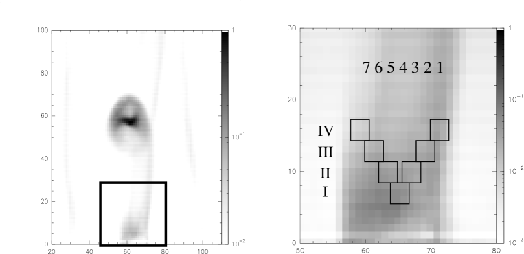
Figure 2: left) An [O II]$\lambda$6300 line emission map for the M4 model in a region near to the jet inlet, at t=15 years. The coordinates are in units of pixels, and the scale bar indicates the normalized intensity. right) A closer view of the jet base, corresponding to the region indicated by the rectangular box in the left-panel, indicating also the $artificial$ slit positions. Regions I, II, III and IV are successively more distant from the jet inlet, while positions 1, 2, 3, 4, 5, 6 and 7 corresponds to different position across the jet radius. Note that each slit have a superposition of 1 px in the direction transverse to the jet axis. For the sake of clarity, we show in this figure only a few (one or two) of the seven slits for each region. See the text for discussion. [See the electronic edition of Astronomy & Astrophysics for a color version of this figure.]

We define four regions along the jet axis, namely regions I, II, III and IV, at distances from the jet inlet of $0\aas@@fstack{\prime\prime}1$, $0\aas@@fstack{\prime\prime}2$, $0\aas@@fstack{\prime\prime}3$ and $0\aas@@fstack{\prime\prime}4$, respectively (assuming a distance of 140 pc and an inclination angle of 45^∘; see §2). For each one of these regions, we construct seven $0\aas@@fstack{\prime\prime}1\times 0\aas@@fstack{\prime\prime}1$ slits (as described above), that are placed side by side parallel to the jet axis with one of them lying exactly on the jet axis (in order to have slits symmetrically disposed on each side of the jet). This configuration (seven aligned slits across the jet beam and in four regions along the jet beam) was chosen in order to mimic the observational conditions described in Bacciotti et al. (bacci02 (2002)). In Figure 2 we show the slits and their positions on the plane of the sky. We note that, in fact, there is an overlap of 1 pixel ($\approx 0\aas@@fstack{\prime\prime}07$) between the slits in each region (see Figure 2).

In Figure 3a, we show the H$\alpha$ line profiles for region IV of model M4 at $t=10$ yr. We note the presence of at least three components in several of the line profiles shown in Figure 3. The emission in the radial velocity range from $\approx$ 0 to $\approx$ -100 km s^-1 is related to the leading bow shock, which surrounds the jet beam. We assume that the emission in the interval from -300 km s^-1 to -100 km s^-1 is related to two components, namely, the high- and medium-velocity components (hereafter, HVC and MVC, respectively). We have performed standard minimum $\chi^{2}$-Gaussian fits to obtain the MVC, for the seven slits in each of the four regions defined in Figure 2. Figure 3b shows the data (full line) combined with the gaussian fit (crosses) for the whole radial velocity interval (left) and for the radial velocity interval ranging from -300 km s^-1 to -100 km s^-1 (right). We also show the gaussian fits decomposing the HVC and MVC. We have performed these fits for all models in Table 1, and for different evolutionary times. This procedure allows us to investigate both the behaviour of the MVC for each emission line as well as its dependence with the imposed initial conditions.

Two distinct evolutionary times were chosen in order to investigate the influence of the presence of an internal working surface (IWS) close to the region where the the slits were placed. In particular, at $t=10$ years (see Fig. 1), an IWS is just being formed (close to the jet inlet, in regions I-IV) due to the chosen $\tau_{pul}=8$ years. On the other hand, for $t=15$ years, the regions I-IV are spatially detached from the position of the nearest IWS (see Fig. 2). In Figure 4 we show the radial velocity of the MVC for regions I, II, III and IV (from top to bottom) as a function of distance from the jet axis (from $-0\aas@@fstack{\prime\prime}2$ to $0\aas@@fstack{\prime\prime}2$; the 0 in the abscissa corresponding to the position of the jet axis) for $t=10$ years (left) and $t=15$ years (right). The radial velocity of the MVC was extracted from the profiles of the H$\alpha$, [O I]$\lambda$6300, [S II]$\lambda$6716 and [N II]$\lambda$6548 emission lines, using the procedure described above. Although the MVC from different emission lines shows slightly different behavior, the distribution of the radial velocity on both sides of the jet axis for a given emission line is perfectly symmetric for the M1 model, regardless the analyzed region or evolutionary time, as we can see clearly in Figure 4.

In Figure 5 we show the radial velocity ($V_{rad}$; left) for regions I, II, III and IV (from top to bottom) of model M2 (with precession but with no rotation) as a function of distance from the jet axis (from $-0\aas@@fstack{\prime\prime}3$ to $0\aas@@fstack{\prime\prime}3$; as in the previous diagram), as well as the difference ($\Delta V_{rad}$) between the radial velocity taken at symmetrical positions with respect to the jet axis (right), at $t=10$ years (top diagrams) and $t=15$ years (bottom diagrams). The precession of the jet axis introduces an asymmetry in the radial velocities as a function of distance from the jet axis, as we can see in the left diagrams of Figure 5. This effect is more pronounced at $t=10$ years, as indicated by the difference in the radial velocities, $\Delta V_{rad}$, in Fig. 5 (top right diagram), and this is due to the presence of an IWS close to regions I-IV. However, such an asymmetry in the distribution of the radial velocity is still present at $t=15$ years. As we can see in Figure 5 (bottom diagrams), $\Delta V_{rad}$ is systematically negative for most of the computed emission lines. Although we cannot establish an unique behaviour for all of the computed lines (considering the distinct regions and evolutionary times), we note that some of them show a clear trend of smaller $\Delta V_{rad}$ for smaller distances from the jet axis ($V_{rad,3}-V_{rad,5}<V_{rad,2}-V_{rad,6}<V_{rad,1}-V_{rad,7}$).

In Figure 6 we again show the radial velocity ($V_{rad}$; left) as a function of distance from the jet axis for regions I, II, III and IV (from top to bottom), as well as the difference ($\Delta V_{rad}$) between the radial velocity taken at symmetrical positions with respect to the jet axis (right), at $t=10$ years (top diagrams) and $t=15$ years (bottom diagrams), but now for model M3. This model presents variability in the velocity of injection as well as an initially imposed rotational profile inside the jet beam, but has no precession (see §2 and Table 1). The asymmetry in the radial velocity distribution, with respect to the jet axis, can be clearly seen in Fig. 6. In particular, $\Delta V_{rad}$ is negative for almost all emission lines, regions and evolutionary stages (with the exception of the [N II]$\lambda$6548 emission line, at $t=10$ years in region II). However, in opposition to model M2, $\Delta V_{rad}$ appears to be greater for smaller distances from the jet axis (at least for some emission lines).

We present the radial velocity distribution for model M4 in Figure 7. Model M4 has variability in both direction and velocity of injection, as well as an initially imposed rotation profile inside the jet beam (see Table 1). The asymmetry in the radial velocity distribution on both sides of the jet axis is more pronounced than in models M2 and M3. This is clearly seen from the radial velocity difference diagrams (right panels in Figure 7), which show $\Delta V_{rad}$ of the order of 0 up to $\approx$ -80 km s^-1. As in model M2, there is a general trend in the $\Delta V_{rad}$ data that shows that it increases as a function of distance from the jet axis, although such a trend is not followed by the H$\alpha$, [O I]$\lambda$6300 and [S II]$\lambda$6716 emission lines in region IV at $t=10$ years and region I at $t=15$ years (see the right diagrams of Figure 7).

In Figure 8 we show the radial velocity shift as a function of distance from the jet axis for regions I to IV (from top to bottom), and for models M1 (crosses), M2 (asterisks), M3 (diamonds) and M4 (squares), for $t=10$ years (left) and $t=15$ years (right). Each point in this diagram corresponds to a mean value for the radial velocity shifts, assuming that $\Delta V_{rad}=\sum_{l=1}^{4}\Delta V_{rad,l}/4$, where the different values of $l$ indicate the H$\alpha$, [O I]$\lambda$6300, [N II]$\lambda$6548 and [S II]$\lambda$6716 emission lines. We clearly see a general trend of increasing radial velocity shifts for larger distances from the jet axis, followed by all the models (with the expected exception of model M1, which shows a null $\Delta V$, as discussed previously). Such a trend is similar to the one discussed in Pesenti et al. (pesenti (2004)) for their disk solution model (and also followed in part by the data of Bacciotti et al bacci02 (2002)).

4 Discussion and conclusions

We have presented a set of 3D numerical simulations of variable velocity jets, from which we have obtained detailed predictions of the emission line profiles of a set of emission lines (H$\alpha$, [O I]$\lambda$6300, [S II]$\lambda$6716 and [N II]$\lambda$6548). The models include an axisymmetric jet, a precessing jet, a rotating jet, and, finally a jet with both precession and rotation (see Table 1 and section 2).

Following Bacciotti et al. (bacci02 (2002)), we carry out double-Gaussian fits to the line profiles, and then study the behaviour of the radial velocity of the MVC (medium velocity component) as a function of distance from the jet axis, for several positions along the jet flow. We find that while the axisymmetric model of course predicts radial velocities whith a symmetric behaviour on both sides of the jet axis, the other three models predict asymmetric behaviours.

The models with precession and with rotation predict systematic offsets of $|\Delta V_{rad}|\lesssim 20$ km s^-1 for the MVC between symmetric positions on both sides of the jet axis. These systematic offsets are seen at most positions along the jet axis, and for many of the emission lines. The magnitudes of these offsets are similar to the ones observed (for many positions and emission lines) by Bacciotti et al. (bacci02 (2002)), Coffey et al. (coffey04 (2004)) and Woitas et al. (woitas05 (2005)). In the model with both precession and rotation (in which the precession was assumed to have a prograde direction), the two effects combine to give larger offsets of $\sim 40-80$ km s^-1.

We have also computed a model with rotation and a retrograde precession. This model (not presented in this paper) produces side-to-side offsets in the MVC radial velocity which are much smaller, and which do not show clear trends as a function of distance from the jet axis.

From these results, we conclude that the radial velocity asymmetries observed in the DG Tau, TH28, RW Aur and LkH$\alpha$321 microjets (see Bacciotti et al. bacci02 (2002); Coffey et al. coffey04 (2004); Woitas et al. woitas05 (2005)) can be modeled either as due to a rotation of the gas in the initial jet cross section, or as due to a precession of the ejection direction. Interestingly, though a precession results in a point-symmetry in the “precession spiral” morphology of the jet beam, the direction of the resulting rotation of the ejected material is of course the same one for both the jet and the counterjet. Also, a “precession spiral” morphology can be produced by an orbital motion of the source around a binary companion (Masciadri & Raga masb (2002); González & Raga gon04c (2004)), resulting in similar radial velocity patterns, but with a morphology with mirror symmetry between the jet and the counterjet.

It is therefore unclear at this time whether the systematic radial velocity asymmetries observed by Bacciotti et al. (bacci02 (2002)), Coffey et al. (coffey04 (2004)) and Woitas et al. (woitas05 (2005)) in the cross sections of several microjets are due to jet rotation or precession (or to a combination of both effects). In order to proceed further, it will be necessary to proceed with more detailed modelling, in which not only the radial velocity asymmetries are considered. A study which also considers the locci of the jet and counterjet on the plane of the sky, resulting in models which simultaneously reproduce the morphology and the radial velocity structure of the observed outflows, might be able to solve this problem. Of the four microjets observed by Bacciotti et al. (bacci02 (2002)), Coffey et al. (coffey04 (2004)) and Woitas et al. (woitas05 (2005)), the jet from RW Aurigae shows the chain of knots with the best alignment. Because of this lack of evidence for a precession spiral structure in the jet beam, the RW Aur jet is probably the most certain case for an observed rotation of the jet beam.

Interestingly, the referee has pointed out to us the very recent results of Cabrit et al. (cabrit05 (2005)), who detect a disk around RW Aur rotating in the opposite sense of the “jet rotation” seen by Woitas et al. (woitas05 (2005)). This result in principle eliminates a jet rotation interpretation for the side-to-side radial velocity asymmetries observed in the RW Aur jet. Therefore, the remaining possibilities are that the jet is precessing (producing the asymmetries explored above), or that it has another intrinsic side-to-side asymmetry (see, e. g., Soker 2005 and Cabrit et al. 2005).

Figure 3: a) H$\alpha$ line profile for model M4, at $t=10$ years, for region 4 (see Figure 2 for slit and region definitions). The slit number is given on the top-right corner of each diagram. The intensity is in units of $10^{-6}$ erg cm^-2 s^-1. b) Left: The H$\alpha$ line profile of slit 4, region IV (full line), superimposed with a three-component $\chi^{2}$-gaussian fit (crosses). Right: a closer viewer of the line profile in the range of -300 to -100 km s^-1, showing the two gaussians (crosses) defined as the high- and medium-velocity components (HVC and MVC, respectively). See the text for a discussion.

Figure 4: Radial velocity as a function of distance from the jet axis for regions I to IV (from top to bottom), for $t=10$ years (left) and $t=15$ years (right) and model M1 (see Table 1). The distance is in units of arcsec, considering a distance of 140 pc from the jet (the zero corresponds to the jet axis position, and the scale, ranging from negative to positive values, corresponds to slits 1 to 7, respectively). The radial velocity is in units of km s^-1. The MVC were extracted from the line profiles for the H$\alpha$, [O I]$\lambda$6300, [S II]$\lambda$6716 and [N II]$\lambda$6548 lines (whose symbols are on the top part of the diagram; we note that, in this diagram, [O I]=[O I]$\lambda$6300, [S II]=[S II]$\lambda$6716 and [N II]=[N II]$\lambda$6548). See the text for a discussion.

Figure 5: Left) The same as in Figure 4, but for the M2 model (see Table 1) at $t=10$ years (top) and $t=15$ years (bottom). The symbols and the scales are the same as in Fig. 4. Right) The radial velocity difference between symmetrically disposed slits (with respect to the jet axis, slit 4; see Figure 2), for $t=10$ years (top) and $t=15$ years (bottom). We note that $\Delta V_{rad}=V_{rad,i}-V_{rad,j}$, where $i=1,2,3$ and $j=7,6,5$ define the slits according to the definition in Figure 2.

Figure 6: The same as in Figure 5, but for the M3 model (see Table 1).

Figure 7: The same as in Figure 5, but for the M4 model (see Table 1).

Figure 8: The radial shift as a function of the distance from the jet axis for regions I, II, III and IV (from top to bottom), for models M1 (crosses), M2 (asterisks), M3 (diamonds) and M4 (squares), for $t=10$ years (left) and $t=15$ years (right).

- (1) Bacciotti, F., Ray, T.P., Mundt, R., Eislöfel, J., & Solf, J. 2002, ApJ, 576, 222
- (2) Blandford, R.D. & Payne, D.G. 1982, MNRAS, 199, 1982
- (3) Cabrit, S., Pety, J., Pesenti, N., Dougados, C. 2005, in Protostars and Planets V (section: Disks and disk accretion) http://www.lpi.usra.edu/meetings/ppv2005/pdf/8103.pdf
- Cantó (1980) Cantó, J., 1980, A&A, 86, 327
- (5) Casse, F., & Ferreira, J. 2000a, A&A, 353, 1115
- (6) Casse, F., & Ferreira, J. 2000b, A&A, 361, 1178
- (7) Cerqueira, A.H., & de Gouveia Dal Pino, E.M. 2004, A&A, 426, L25
- (8) Coffey, D., Bacciotti, F., Woitas, J., Ray, T.P., & Eislöffel, J. 2004, ApJ, 604, 758
- (9) Dougados, C., Cabrit, S., Lavalley, C., & Ménard, F. 2000, A&A, 357, L61
- (10) Ferreira, J. 1997, A&A, 319, 340
- (11) González, R.F., de Gouveia Dal Pino, E.M., Raga, A.C. & Velázquez, P.F. 2004a, ApJ, 616, 976.
- (12) González, R.F., de Gouveia Dal Pino, E.M., Raga, A.C., & Velázquez, P.F. 2004b, ApJ, 600, L59.
- (13) González, R.F. & Raga, A.C. 2004, RMxAA, 40, 61
- Hartmann et al. (1982) Hartmann, L. & MacGregor, K. B., 1982, ApJ, 259, 180
- Kenyon, Dobrzycka, & Hartmann (1994) Kenyon, S.J., Dobrzycka, D., & Hartmann, L, 1994, AJ, 108, 1872
- (16) Lavalley-Fouquet, C., Cabrit, & S., Dougados, C. 2000, A&A, 356, L41
- (17) Masciadri, E. & Raga, A.C. 2002, ApJ, 568, 733
- (18) Masciadri, E., Velázquez, P.F., Raga, A.C., Cantó, J. & Noriega-Crespo, A. 2002, ApJ, 573, 260.
- (19) Mendoza, C. 1983, in Planetary Nebulae, IAUS, 103, 143
- (20) Pesenti, N., Dougados, C., Cabrit, S., Ferreira, J., Casse, F., Garcia, P., O′Brien, D. 2004, A&A, 416, L9
- (21) Pyo, T.-S., Kobayashi, N., Hayashi, M., et al. 2003, ApJ, 590, 340
- (22) Raga, A.C., Navarro-González, R., & Villagran-Muniz, M. 2000, RMxAA, 36, 67
- (23) Raga, A.C., Velázquez, P.F., Cantó, J., Masciadri, E. & Rodríguez, L.F. 2001a, ApJ, 559, 33.
- (24) Raga, A., Sobral, H., Villagrán-Muniz, M., Navarro-González, R. & Masciadri, E. 2001b, MNRAS, 324, 206
- (25) Raga, A., Cabrit, S., Dougados, C., & Lavalley, C. 2001c, A&A, 367, 959
- (26) Raga, A.C., de Gouveia Dal Pino, E. M., Noriega-Crespo, A., Mininni, P. D. & Velázquez, P. F. 2002, A&A, 392, 267
- (27) Raga, A.C., Noriega-Crespo, A., González, R.F. & Velázquez, P.F. 2004, ApJS, 154, 346
- (28) Shu, F., Najita, J., Ostriker, E., Wilkin, F., Ruden, S. & Lizano, S. 1994, ApJ, 429, 781
- (29) Sobral, H., Villagrán-Muniz, M., Navarro-González, R. & Raga, A.C. 2000, Aplied Physics Letters, 77, 3158.
- (30) Soker, N. 2005, A&A, 435, 125
- (31) Testi, L., Bacciotti, F., Sargen, A.I., Ray, T.P., & Eislöffel, J. 2002, A&A, 394, L31
- (32) Van Leer, B. 1982, ICASE Report No. 82-30.
- (33) Velázquez, P.F., Riera, A. & Raga, A.C. 2004, A&A, 419
- (34) Velázquez, P.F., Martinell, J.J., Raga, A.C. & Giacani, E. B. 2004, ApJ, 601, 885
- (35) Velázquez, P.F., de la Fuente, E., Rosado, M. & Raga, A.C. 2001, A&A, 377, 1136
- (36) Velázquez, P.F., Sobral, H., Raga, A.C., Villagrán-Muniz, M. & Navarro-González, R. 2001, RMxAA, 37, 87
- (37) Woitas, J., Ray, T.P., Bacciotti, F., Davis, C.J., & Eislöffel, J. 2002, ApJ, 580, 336
- (38) Woitas, J., Bacciotti, F., Ray, T.P., Marconi, A., Coffey, D., & Eislöffel, J. 2005, A&A, 432, 149