The theory of spectral evolution of the GRB prompt emission

Abstract

We develop the theory of jitter radiation from GRB shocks containing small-scale magnetic fields and propagating at an angle with respect to the line of sight. We demonstrate that the spectra vary considerably: the low-energy photon index, $\alpha$, ranges from $0$ to $-1$ as the apparent viewing angle goes from $0$ to $\pi/2$. Thus, we interpret the hard-to-soft evolution and the correlation of $\alpha$ with the photon flux observed in GRBs as a combined effect of temporal variation of the viewing angle and relativistic aberration of an individual thin, instantaneously illuminated shell. The model predicts that about a quarter of time-resolved spectra should have hard spectra, violating the synchrotron $\alpha=-2/3$ line of death. The model also naturally explains why the peak of the distribution of $\alpha$ is at $\alpha\approx-1$. The presence of a low-energy break in the jitter spectrum at oblique angles also explains the appearance of a soft X-ray component in some GRBs and a relatively small number of them. We emphasize that our theory is based solely on the first principles and contains no ad hoc (phenomenological) assumptions.

1. Introduction

Rapid spectral variability is a remarkable, yet unexplained feature of the prompt GRB emission. The variation of the hardness of the spectrum and the hard-to-soft evolution are the most acknowledged features (Bhat, et al. 1994; Crider, et al. 1997; Frontera, et al. 2000; Ryde & Petrosian 2002). A quite remarkable “tracking” behavior, when the low-energy spectral index $\alpha$ follows (or correlates with) the photon flux (Crider, et al. 1997) is particularly intriguing. An example of such trend is shown in Fig. 1 (we used data from Preece, et al. 2000).

In this paper, we demonstrate that the spectral index–flux correlation (or the hardness-intensity correlation) is a natural and inevitable prediction of the collisionless relativistic shock model and the jitter radiation mechanism from small-scale shock-generated magnetic fields (Medvedev & Loeb 1999; Medvedev 2000). Quite possibly, the appearance of a soft X-ray component in some GRBs (Preece, et al. 1995) can also be interpreted within this model. The theory yields a right number of the synchrotron-violating GRBs, i.e., with $\alpha>-2/3$, (Katz 1994; Preece, et al. 1998) and naturally explains why the majority of GRBs have $\alpha$ around $-1$ (Preece, et al. 2000). We emphasize that our theory is based solely on the first principles and contains no ad hoc assumptions.

2. Theory of jitter radiation in 3D

The angle-averaged spectral power emitted by a relativistic particle moving through small-scale random magnetic fields, under the assumption that the deflection angle is negligible and the particle trajectory is a straight line, has been derived elsewhere (Rybicki & Lightman 1979; Landau & Lifshitz 1971; Medvedev 2000) and it reads

$$\frac{dW}{d\omega}=\frac{e^{2}\omega}{2\pi c^{3}}\int_{\omega/2\gamma^{2}}^{\infty}\frac{\left|{\bf w}_{\omega^{\prime}}\right|^{2}}{\omega^{\prime 2}}\left(1-\frac{\omega}{\omega^{\prime}\gamma^{2}}+\frac{\omega^{2}}{2\omega^{\prime 2}\gamma^{4}}\right)\,d\omega^{\prime},$$ (1)

where we neglect plasma dispersion, which is vanishing for the GRB photons. Here $\gamma$ is the Lorentz factor of a radiating particle and ${\bf w}_{\omega^{\prime}}=\int{\bf w}e^{i\omega^{\prime}t}\,dt$ is the Fourier component of the transverse particle’s acceleration due to the Lorentz force, $F_{L}$. This temporal Fourier transform is taken along the particle trajectory, ${\bf r}={\bf r}_{0}+{\bf v}t$. It should appropriately be expressed via the statistical properties of the magnetic field. To make this section self-contained, we will, in part, follow the derivation of Fleishman (2005).

We need to express the temporal Fourier component of the acceleration ${\bf w}\equiv F_{L}/\gamma m$ taken along the particle trajectory in terms of the Fourier component of the field in the spatial and temporal domains. Taking the Fourier transform of ${\bf w}({\bf r}_{0}+{\bf v}t,t)$, we have

$${\bf w}_{\omega^{\prime}} = (2\pi)^{-4}\int e^{i\omega^{\prime}t}\,dt\left(e^{-i(\Omega t-{\bf k\cdot r}_{0}-{\bf k\cdot v}t)}{\bf w}_{\Omega,{\bf k}}\,d\Omega d{\bf k}\right)$$ (2)

$$= (2\pi)^{-3}\int{\bf w}_{\Omega,{\bf k}}\delta(\omega^{\prime}-\Omega+{\bf k\cdot v})\,e^{i{\bf k\cdot r}_{0}}\,d\Omega d{\bf k},$$

where we used that $\int e^{i\omega t}\,dt=2\pi\delta(\omega)$. In a statistically homogeneous turbulence, $|{\bf w}_{\omega^{\prime}}|^{2}$ should not depend on the initial point, ${\bf r}_{0}$, of the particle trajectory. Therefore, we average it over ${\bf r}_{0}$ as $\langle|{\bf w}_{\omega^{\prime}}|^{2}\rangle=V^{-1}\int|{\bf w}_{\omega^{\prime}}|^{2}d{\bf r}_{0}$, where $V$ is the volume of the spatial domain. Using that $\int e^{i({\bf k-k}_{1})\cdot{\bf r}_{0}}\,d{\bf r}_{0}=(2\pi)^{3}\delta({\bf k-k}_{1})$, we finally have:

$$\langle|{\bf w}_{\omega^{\prime}}|^{2}\rangle=(2\pi)^{-3}V^{-1}\int|{\bf w}_{\Omega,{\bf k}}|^{2}\delta(\omega^{\prime}-\Omega+{\bf k\cdot v})\,d\Omega d{\bf k}.$$ (3)

The Lorentz acceleration, ${\bf w}=(e/\gamma mc){\bf v\times B}$, can be written as $w_{\alpha}=(e/\gamma mc)\frac{1}{2}e_{\alpha\beta\gamma}(v_{\beta}B_{\gamma}-v_{\gamma}B_{\beta})$. Using the identity, $e_{\alpha\beta\gamma}e_{\alpha\lambda\mu}=\delta_{\beta\lambda}\delta_{\gamma\mu}-\delta_{\beta\mu}\delta_{\gamma\lambda}$, we obtain

$$|{\bf w}_{\Omega,{\bf k}}|^{2}=(ev/\gamma mc)^{2}(\delta_{\alpha\beta}-v^{-2}v_{\alpha}v_{\beta})\,B_{\Omega,{\bf k}}^{\alpha}B_{\Omega,{\bf k}}^{*\beta}.$$ (4)

In a statistically homogeneous random magnetic field, the tensor $B_{\Omega,{\bf k}}^{\alpha}B_{\Omega,{\bf k}}^{*\beta}$ can be expressed via the Fourier transform of the field correlation tensor

$$B_{\Omega,{\bf k}}^{\alpha}B_{\Omega,{\bf k}}^{*\beta}=TVK_{\alpha\beta}(\Omega,{\bf k})=TV\!\!\!\int\!\!e^{i(\Omega t-{\bf k\cdot r})}K_{\alpha\beta}({\bf r},t)\,d{\bf r}dt,$$ (5)

where $T$ is the size of the temporal domain and $K_{\alpha\beta}({\bf r},t)=T^{-1}V^{-1}\int B_{\alpha}({\bf r}^{\prime},t^{\prime})B_{\beta}({\bf r^{\prime}+r},t^{\prime}+t)\,d{\bf r}^{\prime}dt$ is the second-order correlation tensor of the magnetic field (Fleishman 2005).

In the static case, i.e., when the magnetic field is independent of time, Eqs. (3), (4) read as

$$\langle|{\bf w}_{\omega^{\prime}}|^{2}\rangle = (2\pi V)^{-1}\int|{\bf w}_{\bf k}|^{2}\delta(\omega^{\prime}+{\bf k\cdot v})\,d{\bf k},$$ (6)

$$|{\bf w}_{\bf k}|^{2} = (ev/\gamma mc)^{2}(\delta_{\alpha\beta}-v^{-2}v_{\alpha}v_{\beta})\,VK_{\alpha\beta}({\bf k}).$$ (7)

3. The magnetic field spectrum

We adopt the following geometry: a shock is located in the $x$-$y$-plane and is propagating along $z$-direction. As it has initially been demonstrated by Medvedev & Loeb (1999) and later confirmed via 3D PIC simulations (Silva, et al. 2003; Nishikawa, et al. 2003; Frederiksen, et al. 2004), the magnetic field at relativistic shocks is described by a random vector field in the shock plane, i.e., the $x$-$y$-plane. As the shock is propagating through a medium, the produced field is transported downstream (in the shock frame) whereas new field is continuously generated at the shock front. Thus, the field is also random in the parallel direction, i.e., the $z$-direction. Thus, Weibel turbulence at the shocks is highly anisotropic. Both the theoretical considerations and realistic 3D simulations of relativistic shocks indicate that the dynamics of of the Weibel magnetic fields in the shock plane and along the normal to it are decoupled. Hence, the Fourier spectra of the field in the $x-y$ plane and in $z$ direction are independent. Thus, for the Weibel fields at shocks, the correlation tensor has the form

$$K_{\alpha\beta}({\bf k})=C(\delta_{\alpha\beta}-n_{\alpha}n_{\beta})f_{z}(k_{\|})f_{xy}(k_{\perp}),$$ (8)

where ${\bf n}$ is the unit vector normal to the shock front, $C$ is the normalization constant proportional to $\langle B^{2}\rangle$, $f_{z}$ and $f_{xy}$ are the magnetic field spectra along ${\bf n}$ and in the shock plane, respectively, $k_{\bot}=(k_{x}^{2}+k_{y}^{2})^{1/2}$ and $k_{\|}=k_{z}$, and finally, the tensor $(\delta_{\alpha\beta}-n_{\alpha}n_{\beta})$ is symmetric and its product with ${\bf n}$ is zero, implying orthogonality of $\bf n$ and $\bf B$.

Numerical simulatrions (Frederiksen, et al. 2004) also indicate that the field transverse spectrum, $f_{xy}$, is well described by a broken power-law with the break scale comparable to the skin depth, $c/\omega_{p}$, where $\omega_{p}=(4\pi e^{2}n/\Gamma m)^{1/2}$ is the relativistic plasma frequency and $\Gamma$ is the shock Lorentz factor. We expect that the spectrum $f_{z}$, has similar properties. Therefore, we use the following models:

$$f_{z}(k_{\|})=\frac{k_{\|}^{2\alpha_{1}}}{(\kappa_{\|}^{2}+k_{\|}^{2})^{\beta_{1}}},\quad f_{xy}(k_{\bot})=\frac{k_{\perp}^{2\alpha_{2}}}{(\kappa_{\perp}^{2}+k_{\perp}^{2})^{\beta_{2}}},$$ (9)

where $\kappa_{\|}$ and $\kappa_{\perp}$ are parameters (being, in general, a function of the distance from the front, Medvedev, et al. 2005) determining the location of the peaks in the spectra, $\alpha_{1},\ \alpha_{2},\ \beta_{1},\ \beta_{2}$ are power-law exponents below and above a spectral peak ($\beta_{1}>\alpha_{2}+1/2$ and $\beta_{2}>\alpha_{2}+1$, for convergence at high-$k$). Note that $\beta_{1,2}\to\infty$ corresponds to spectra with a sharp cut-off. The asymptotes of these functions are

$$f(k)\propto\left\{\begin{array}[]{ll}k^{2\alpha},&\textrm{if }k\ll\kappa,\\ k^{2\alpha-2\beta},&\textrm{if }k\gg\kappa.\end{array}\right.$$ (10)

4. Radiation spectra from a shock viewed at different angles

We now evaluate Eqs. (6),(7). The scalar product of the two tensors is

$$(\delta_{\alpha\beta}-v_{\alpha}v_{\beta}/v^{2})(\delta_{\alpha\beta}-n_{\alpha}n_{\beta})=1+(n_{\alpha}v_{\alpha})^{2}/v^{2}=1+\cos^{2}\Theta,$$ (11)

where we used that $\delta_{\alpha\alpha}=3$. Here $\Theta$ is the angle between the normal to the shock and the particle velocity (in an observer’s frame), which is approximately the direction toward an observer, that is ${\bf v\|k}$ for an ultra-relativistic particle (because of relativistic beaming, the emitted radiation is localized within a narrow cone of angle $\sim 1/\gamma$). Eq. (6) becomes

$$\langle|{\bf w}_{\omega^{\prime}}|^{2}\rangle=\frac{C}{2\pi}\,(1+\cos^{2}\Theta)\int\!\!f_{z}(k_{\|})f_{xy}(k_{\perp})\delta(\omega^{\prime}+{\bf k\cdot v})\,dk_{\|}d^{2}k_{\perp}.$$ (12)

Equations (1),(12) fully determine the spectrum of jitter radiation from a GRB shock. We now consider special cases.

4.1. A shock viewed head-on, $\Theta=0$

For a shock moving towards an observer, ${\bf n\|k}$, hence $\Theta=0$ (because $\bf n\|v$ and $\bf k\|v$ for $\gamma\gg 1$) and ${\bf k\cdot v}=k_{z}v$ (of course, $v\approx c$). Equation (12) then reads

$$\langle|{\bf w}_{\omega^{\prime}}|^{2}\rangle = \pi^{-1}C\,\overline{f_{xy}}\,\int f_{z}(k_{z})\delta(\omega^{\prime}+k_{z}v)\,dk_{z}$$ (13)

$$= (C/\pi|v|)\,\overline{f_{xy}}\,f_{z}(-\omega^{\prime}/v),$$

where $\overline{f_{xy}}=\int f_{xy}(k_{\perp})d^{2}k_{\perp}$. Apparently, this case is analogous to the 1D model used by Medvedev (2000). We now determine low-$\omega$ and high-$\omega$ asymptotics for the spectrum given by Eq. (9). In order to simplify the analysis, we neglect the small second and third terms in the brackets in Eq.(1) and assume that $\alpha_{1}>1/2,\ \beta_{1}>1$. This slightly changes the shape of the radiation spectrum near a peak, but does not affect the asymptotic behavior. We have

$$\frac{dW}{d\omega}\propto\omega^{2\alpha_{1}-2\beta_{1}}\int_{y_{0}}^{\infty}\frac{y^{2\alpha_{1}}}{(\eta_{\|}^{2}+y^{2})^{\beta_{1}}}\,\frac{dy}{y^{2}},$$ (14)

where $y=\omega^{\prime}/\omega$, $\eta_{\|}=\kappa_{\|}v/\omega$, and $y_{0}=1/2\gamma^{2}$.

At low frequencies, $\eta_{\|}\gg y_{0}$, (that is, $\omega\ll\kappa_{\|}v\gamma^{2}$), the right hand side of Eq. (14) can approximately be evaluated as $\textrm{RHS}\sim\omega^{2\alpha_{1}-2\beta_{1}}(\int_{0}^{\eta_{\|}}y^{2\alpha_{1}-2}\eta_{\|}^{-2\beta_{1}}dy+\int_{\eta_{\|}}^{\infty}y^{2\alpha_{1}-2-2\beta_{1}}dy)\propto\omega^{2\alpha_{1}-2\beta_{1}}\eta_{\|}^{2\alpha_{1}-1-2\beta_{1}}\propto\omega^{1}$. At high frequencies $\eta_{\|}\ll y_{0}$, (that is, $\omega\gg\kappa_{\|}v\gamma^{2}$), the right hand side becomes (note, $y_{0}=const.$) $\textrm{RHS}\sim\omega^{2\alpha_{1}-2\beta_{1}}\int_{y_{0}}^{\infty}y^{2\alpha_{1}-2-2\beta_{1}}dy\propto\omega^{2\alpha_{1}-2\beta_{1}}$. Combining the results, we conclude that

$$\left.\frac{dW}{d\omega}\right|_{\Theta=0}\propto\left\{\begin{array}[]{ll}\omega^{1},&\textrm{if }\omega\ll\kappa_{\|}v\gamma^{2},\\ \omega^{2\alpha_{1}-2\beta_{1}},&\textrm{if }\omega\gg\kappa_{\|}v\gamma^{2}.\end{array}\right.$$ (15)

4.2. A shock viewed edge-on, $\Theta=\pi/2$

An ultra-relativistic shock moving at an angle $\sim 1/\Gamma$ with respect to the line of sight is seen nearly edge-on because of relativistic aberration. In this case, the shock is seen as if ${\bf n\perp k}$. Therefore $\Theta=\pi/2$ and ${\bf k\cdot v}=k_{x}v$, where we assumed that an observer is located on the $x$-axis. Equation (12) then becomes

$$\langle|{\bf w}_{\omega^{\prime}}|^{2}\rangle = (2\pi)^{-1}C\,\overline{f_{z}}\,\int f_{xy}(k_{\perp})\delta(\omega^{\prime}+k_{x}v)\,dk_{x}dk_{y}$$ (16)

$$= (C/2\pi|v|)\,\overline{f_{z}}\,\int f_{xy}(\sqrt{(\omega^{\prime}/v)^{2}+k_{y}^{2}})\,dk_{y}$$

$$\propto (\omega^{\prime})^{2\alpha_{2}-2\beta_{2}+1}\int_{0}^{\infty}\frac{(1+y^{2})^{\alpha_{2}}}{(\eta_{*}^{2}+1+y^{2})^{\beta_{2}}}\,dy,$$

where $\overline{f_{z}}=\int f_{z}(k_{\|})dk_{\|}$. In the last line, we introduced $y=k_{y}v/\omega^{\prime}$ and $\eta_{*}=\kappa_{\perp}v/\omega^{\prime}$. The integral in Eq. (16) is independent of $\omega^{\prime}$ when $\eta_{*}\ll 1$, i.e., at high frequencies, $\omega^{\prime}\gg\kappa_{\perp}v$. At low frequencies, $\eta_{*}\gg 1$, the integral is dominated by $y\sim\eta_{*}$ (as in Eq. [14]), hence it is $\propto\eta_{*}^{2\alpha_{2}-2\beta_{2}+1}\propto\omega^{\prime-(2\alpha_{2}-2\beta_{2}+1)}$. Thus, we have

$$\langle|{\bf w}_{\omega^{\prime}}|^{2}\rangle\propto\left\{\begin{array}[]{ll}(\omega^{\prime})^{0},&\textrm{if }\omega^{\prime}\ll\kappa_{\perp}v,\\ (\omega^{\prime})^{2\alpha_{2}-2\beta_{2}+1},&\textrm{if }\omega^{\prime}\gg\kappa_{\perp}v.\end{array}\right.$$ (17)

Comparing Eqs. (17) and (10), we approximate $\langle|{\bf w}_{\omega^{\prime}}|^{2}\rangle$ by a function as in Eq. (9) with $\alpha=0$ and $-2\beta=2\alpha_{2}-2\beta_{2}+1$. We can now find the asymptotes of the spectra from Eq. (1). The analysis is analogous to that of Eq. (14) and it yields

$$\left.\frac{dW}{d\omega}\right|_{\Theta=\pi/2}\propto\left\{\begin{array}[]{ll}\omega^{0},&\textrm{if }\omega\ll\kappa_{\perp}v\gamma^{2},\\ \omega^{2\alpha_{2}-2\beta_{2}+1},&\textrm{if }\omega\gg\kappa_{\perp}v\gamma^{2}.\end{array}\right.$$ (18)

This result is analogous to that of Fleishman (2005).

4.3. A shock viewed at oblique angles, $0<\Theta<\pi/2$

For a shock viewed at an oblique angle, ${\bf k}={\bf\hat{x}}k\sin\Theta+{\bf\hat{z}}k\cos\Theta$, we have ${\bf k\cdot v}=k_{x}v\sin\Theta+k_{z}v\cos\Theta$. Hence

$$\langle|{\bf w}_{\omega^{\prime}}|^{2}\rangle = \frac{C}{2\pi}\,\int f_{z}(k_{z})f_{x\bar{y}}(k_{x})\delta(\omega^{\prime}+{\bf k\cdot v})\,dk_{z}dk_{x}$$ (19)

$$= C_{*}\,\int f_{z}\!\left(\frac{\omega^{\prime}/v}{\cos\Theta}+k_{x}\tan\Theta\right)f_{x\bar{y}}(k_{x})\,dk_{x},$$

$$\propto (\omega^{\prime})^{\zeta}\int_{-\infty}^{\infty}\frac{(1+y)^{2\alpha_{1}}}{[\eta_{1}^{2}+(1+y)^{2}]^{\beta_{1}}}\frac{y^{2\alpha_{2}}\,dy}{(\eta_{2}^{2}+y^{2})^{\beta_{2}}},$$

where we used that $f_{z}(-k_{z})=f_{z}(k_{z})$ and we defined $C_{*}=C/(2\pi|v\cos\Theta|)$ and $f_{x\bar{y}}(k_{x})=\int f_{xy}((k_{x}^{2}+k_{y}^{2})^{1/2})dk_{y}$. One can show that this function is very similar to $f_{xy}(k_{\perp})$ with $k_{\perp}$ replaced with $k_{x}$, so we use it in our analysis. In the last line we introduced $\zeta=2\alpha_{1}-2\beta_{1}+2\alpha_{2}-2\beta_{2}+1$, $y=k_{x}v\sin\Theta/\omega^{\prime}$, $\eta_{1}=\kappa_{\|}v\cos\Theta/\omega^{\prime}$, $\eta_{2}=\kappa_{\perp}v\sin\Theta/\omega^{\prime}$. If $\kappa_{\perp}\sim\kappa_{\|}$ and $\Theta\ll 1$, then $\eta_{1}\gg\eta_{2}$ and we can conclude that $\langle|{\bf w}_{\omega^{\prime}}|^{2}\rangle$ has two breaks: $\omega^{\prime}_{1}=\kappa_{\|}v\cos\Theta$ and $\omega^{\prime}_{2}=\kappa_{\perp}v\sin\Theta$. A more detailed numerical analysis and the resulting radiation spectrum are discussed below.

5. Interpretation of prompt GRB spectra

In the standard internal shock model, each emission episode is associated with illumination of a thin shell, — an internal shock and the hot and magnetized post-shock material. We assume that the shell is spherical (at least within a cone of opening angle of $\sim 1/\Gamma$ around the line of sight) and this shell is simultaneously illuminated for a short period of time. The observed photon pulse is broadened because the photons emitted from the patches of the shell located at larger angles, $\vartheta$, from the line of sight arrive at progressively later times (Piran 1999). This effect naturally explains the fast-rise-slow-decay lightcurves of individual pulses (Ryde & Petrosian 2002; Kocevski, et al. 2003). Because of relativistic aberration, the apparent viewing angle, $\Theta$, is greater than $\vartheta$ and approaches $\Theta\sim\pi/2$ (the shell is seen edge-on) when $\vartheta\sim 1/\Gamma$. Thus, there must be a tight correlation between the observed spectrum and the observed photon flux, because they are, in essence, different manifestations of the same relativistic kinematics effect.

Let us now discuss specific properties of the predicted spectra. Fig. 2 represents full numerical solutions of Eqs. (1), (9), (12) for three different viewing angles. In calculation of $dW/d\omega$, the emitting electrons were assumed monoenergetic, for simplicity. The extension to a standard power-law with a sharp low-energy cutoff, $N\sim\gamma^{-p}$ for $\gamma>\gamma_{\rm min}$ is straightforward: the low-$\omega$ spectral slope remains unchanged, and the high-$\omega$ slope is equal to $\zeta$ or $-(p-1)/2$, whichever is greater (neglecting $e^{-}$ cooling). An important fact to note is that the jitter radiation spectrum varies with the viewing angle. When a shock velocity is along the line of sight, the low-energy spectrum is hard $F_{\nu}\propto\nu^{1}$, harder than the “synchrotron line of death” ($F_{\nu}\propto\nu^{1/3}$). As the viewing angle increases, the spectrum softens, and when the shock velocity is orthogonal to the line of sight, it becomes $F_{\nu}\propto\nu^{0}$. Another interesting feature is that at oblique angles, the spectrum does not soften simultaneously at all frequencies. Instead, there appears a smooth spectral break, which position depends on $\Theta$. The spectrum approaches $\sim\nu^{0}$ below the break and is harder above it. This softening of the spectrum at low $\nu$’s could be interpreted as the appearance of an additional soft X-ray component, similar to that found in some of GRBs (Preece, et al. 1995).

Fig. 3 represents the spectral slope evaluated at frequencies about 10 and 30 times below the spectral peak. These frequencies correspond to the edge of the BATSE window for bursts with the peak energy of about 200 keV and 600 keV, respectively. Hence, the spectral slope, $\alpha_{\rm GRB}$, will be close to those obtained from the data fits. Since $\Theta(t)$ increases with time during an individual emission episode, the curves roughly represent the temporal evolution of $\alpha_{\rm GRB}$. Assuming that time-resolved spectra are homogeneously distributed over $\Theta$, one can estimate the relative fraction of the synchrotron-violating GRBs (i.e., those with $\alpha_{\rm GRB}+1>1/3$) as about 25%, which is very close to the 30% obtained from the data (Preece, et al. 2000). Most of the GRBs, $\sim$75%, should, by the same token, be distributed around $\alpha_{\rm GRB}\sim-1$. Note also that time-integrated GRB spectra should have $\alpha_{\rm GRB}$ around minus one, as well. This explains why a relatively large sample of synchrotron-violating bursts is present in the time-resolved BSAX and BATSE data (Preece, et al. 2000; Frontera, et al. 2000). Since time-integrated data are dominated by $\alpha\sim-1$ spectra, the synchrotron-violating GRBs should be practically absent from the time-intergtated BATSE and HETE-II spectral data (Barraud, et al. 2003). We stress that the question of why the peak of the $\alpha_{\rm GRB}$-distribution is at $\alpha_{\rm GRB}=-1$ and not at some other “physically motivated” value of $-3/2$ or $-2/3$, has had no satisfactory explanation until now. Finally, the spectral softening which looks like an additional soft X-ray component should appear within the detector spectral window when $\Theta\sim 20^{\circ}\pm$ few degrees. Thus, we estimate that this X-ray excess can be detectable in about 10% of GRBs, which is again quite close to the observed 15% (Preece, et al. 1995). Of course, a careful statistical analysis, which takes into account uneven sampling (more time-resolved spectra for brighter parts of the bursts), statistical and systematic errors, biases introduced by fits to particular spectral models, etc., is very desirable. However, the very fact that relative sizes of GRB populations fall in the right bulk part is very encouraging.

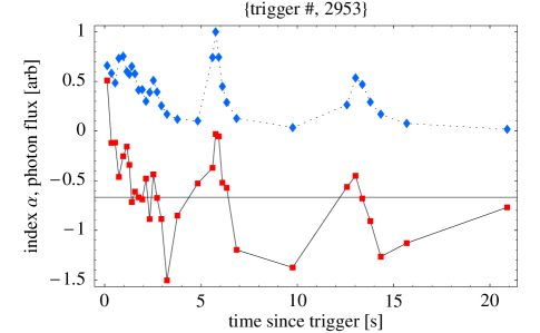
Figure 1.— The normalized photon flux (diamonds) and the low-energy power-law index $\alpha$ (squares) vs time for BATSE trigger #2953. The data are from the time-resolved spectral fits by Preece, et al. (2000).

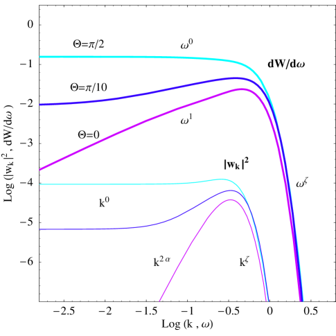
Figure 2.— The $\log-\log$ plots of $|{\bf w_{k}}|^{2}$ vs $k$ (thin lines) and of $dW/d\omega$ vs $\omega$ (thick lines), for three viewing angles $\Theta=0,\ \pi/10,\ \pi/2$. The axes units are arbitrary. In this calculation we used $f_{z}=f_{xy}$ with $\alpha=2,\ \beta=20,\ \kappa=1,\ v=1$. The exponent $\zeta=\zeta(\alpha,\beta)$ is model dependent [c.f., Eqs. (15), (18)]. We also chose $\gamma=1$ in order to align the peaks of $|{\bf w_{k}}|^{2}$ and $dW/d\omega$. Note that the actual peaks are at values $k,\ \omega$ lower than 10 by a factor two or three. Note also that the spectrum $dW/d\omega$ levels off at oblique angles at frequencies much smaller than $\kappa v\gamma^{2}\sin\Theta$, whereas $|{\bf w_{k}}|^{2}$ indeed starts to flatten at $k\sim\kappa v\sin\Theta$.

Figure 3.— The low-energy spectral slope evaluated at $\omega\sim 0.03$ (solid curve) and $\omega\sim 0.01$ (dashed curve) in units of Fig. 2, i.e., at $\omega$’s about 10 and 30 times below the spectral peak, corresponding to the low-$\omega$ edge of the BATSE window for GRBs with $E_{p}$ of about 200 and 600 keV, respectively. Note that abour 25% of spectra violate the synchrotron line of death (solid horizontal line).

References

• Barraud, et al. (2003) Barraud, C., et al. 2003, A&A, 400, 1021
• Bhat, et al. (1994) Bhat, P. N., et al. 1994, ApJ, 426, 604
• Crider, et al. (1997) Crider, A., et al. 1997, ApJ, 479, L39
• Fleishman (2005) Fleishman, G. D. 2005, astro-ph/0502245
• Frederiksen, et al. (2004) Frederiksen, J. T., Hededal, C. B., Haugb$\emptyset$lle, T., & Nordlund, Å. 2004, ApJ, 608, L13
• Frontera, et al. (2000) Frontera, F., et al. 2000, ApJS, 127, 59
• Katz (1994) Katz, J. I. 1995, ApJ, 432, L107
• Kocevski, et al. (2003) Kocevski, D., Ryde, F., Liang, E. 2003, ApJ, 596, 389
• Landau & Lifshitz (1971) Landau, L. D., & Lifshitz, E. M. 1971, The classical theory of fields (Oxford: Pergamon Press)
• Medvedev & Loeb (1999) Medvedev, M. V., & Loeb, A. 1999, ApJ, 526, 697
• Medvedev (2000) Medvedev, M. V. 2000, ApJ, 540, 704
• Medvedev, et al. (2005) Medvedev, M. V., Fiore, M., Fonseca, R. A., Silva, L O., Mori, W. B. 2005, ApJ, 618, L75
• Nishikawa, et al. (2003) Nishikawa, K.-I., Hardee, P., Richardson, G., Preece, R., Sol, H., & Fishman, G. J. 2003, ApJ, 595, 555
• Piran (1999) Piran, T. 1999, Phys. Rep., 314, 575
• Preece, et al. (1995) Preece, R. D., et al. 1995, Ap&SS, 231, 207
• Preece, et al. (1998) Preece, R. D., Briggs, M. S., Malozzi, R. S., Pendleton, G. N., Paciesas, W. S., Band, D. L. 1998, ApJ, 506, 23
• Preece, et al. (2000) Preece, R. D., Briggs, M. S., Mallozzi, R. S., Pendleton, G. N., Paciesas, W. S., Band, D. L. 2000, ApJS, 126, 19
• Rybicki & Lightman (1979) Rybicki, G. B., & Lightman, A. P. 1979, Radiative processes in astrophysics, (New York: Wiley)
• Ryde & Petrosian (2002) Ryde, F. & Petrosian, V. 2002, ApJ, 578, 290
• Silva, et al. (2003) Silva, L. O., Fonseca, R. A., Tonge, J. W., Dawson, J. M., Mori, W. B., & Medvedev, M. V. 2003, ApJ, 596, L121
Refer to caption