Broad-band photometric colors and effective temperature calibrations for late-type giants. I. Z=0.02

We present new synthetic broad-band photometric colors for late-type giants based on synthetic spectra calculated with the PHOENIX model atmosphere code. The grid covers effective temperatures $T_{\rm eff}=3000\dots 5000$ K, gravities $\log g=-0.5\dots+3.5$, and metallicities ${\rm[M/H]}=+0.5\dots-4.0$. We show that individual broad-band photometric colors are strongly affected by model parameters such as molecular opacities, gravity, microturbulent velocity, and stellar mass. Our exploratory 3D modeling of a prototypical late-type giant shows that convection has a noticeable effect on the photometric colors too, as it alters significantly both the vertical and horizontal thermal structures in the outer atmosphere. The differences between colors calculated with full 3D hydrodynamical and 1D model atmospheres are significant (e.g., $\Delta(V-K)\sim 0.2$ mag), translating into offsets in effective temperature of up to $\sim$70 K. For a sample of 74 late-type giants in the Solar neighborhood, with interferometric effective temperatures and broad-band photometry available in the literature, we compare observed colors with a new PHOENIX grid of synthetic photometric colors, as well as with photometric colors calculated with the MARCS and ATLAS model atmosphere codes. We find good agreement of the new synthetic colors with observations and published $T_{\rm eff}$–color and color–color relations, especially in the $T_{\rm eff}$–$(V-K)$, $T_{\rm eff}$–$(J-K)$ and $(J-K)$–$(V-K)$ planes. Deviations from the observed trends in the $T_{\rm eff}$–color planes are generally within $\pm 100$ K for $T_{\rm eff}=3500$ to 4800 K. Synthetic colors calculated with different stellar atmosphere models agree to $\pm 100$ K, within a large range of effective temperatures and gravities. The comparison of the observed and synthetic spectra of late-type giants shows that discrepancies result from the differences both in the strengths of various spectral lines/bands (especially those of molecular bands, such as TiO, H₂O, CO) and the continuum level. Finally, we derive several new $T_{\rm eff}$–$\log g$–color relations for late-type giants at solar-metallicity (valid for $T_{\rm eff}=3500$ to 4800 K), based both on the observed effective temperatures and colors of the nearby giants, and synthetic colors produced with PHOENIX, MARCS and ATLAS model atmospheres.

1 Introduction

During the last decade considerable progress has been made in modeling stellar atmospheres over large ranges of effective temperatures, gravities and metallicities (see, e.g., Hauschildt et al. (2003) and references therein for the PHOENIX models; Castelli & Kurucz (2003) for ATLAS models; Plez (2003) and Gustafsson et al. (2003) for MARCS models). While theoretical spectra show good agreement with observations over a wide area in the HR diagram, late-type giants are still thought to be one of the challenging exceptions (e.g., Bessell et al. 1998).

The contribution from late-type giants on the Red Giant Branch (RGB) and Asymptotic Giant Branch (AGB) is important in many astrophysical contexts related to intermediate-age and old stellar populations, thus correct representation of their atmospheres and spectra is of crucial importance. However, all state-of-art stellar atmosphere models use a number of simplifications related to the physics, and thus it is very important to know how well the different theoretical models (e.g., PHOENIX, MARCS, ATLAS) can reproduce photometric features of real stars, in particular those for which reliable fundamental stellar parameters (such as $T_{\rm eff}$, ${\rm log}\,g$, metallicity) are known.

The contribution of this study is three-fold. We provide a grid of synthetic broad-band photometric colors for late-type giants, based on the new PHOENIX library of synthetic spectra (Hauschildt et al. 2005, in preparation). The new PHOENIX library is an update and extension of the previous NextGen library of synthetic spectra (Hauschildt et al. 1999a, b) to lower effective temperatures and metallicities. The major improvements of the current models with respect to NextGen are updated equation of state data and updated molecular opacities and line list, e.g., water and TiO lines (Sect. 2). The new grid of photometric colors covers $T_{\rm eff}=3000\dots 5000$ K, $\log g=-0.5\dots+3.5$, and $\left[\mathrm{M}/\mathrm{H}\right]=+0.5\dots-4.0$.

We also make a detailed investigation of the influence of model parameters on the resulting broad-band photometric colors, namely, the effects of molecular opacities, gravity, microturbulent velocity, stellar mass, and the treatment of convection. This analysis is done for colors at Solar metallicity and covers a wide range of effective temperatures and gravities typical for late-type giants ($T_{\rm eff}=3000\dots 4800$ K and $\log g=0.0\dots+3.0$). To investigate the effects of convection on the broad-band photometric colors, we calculate a full 3D hydrodynamic model of a prototypical late-type giant ($T_{\rm eff}\simeq 3700\,\mathrm{K}$, $\log g=1.0$, and ${\rm\left[\mathrm{M}/\mathrm{H}\right]}=0.0$) using the 3D model atmosphere code CO⁵BOLD, and provide a comparison of 3D colors with those obtained using a standard 1D model atmosphere.

Finally, we make an extensive comparison of the synthetic broad-band photometric colors with observations of late-type giants, and with empirical as well as theoretical $T_{\rm eff}$–color and color–color relations available from the literature. This comparison is done for colors at Solar metallicity. For this purpose we employ a new PHOENIX grid of synthetic photometric colors, together with colors calculated employing MARCS (Plez 2003, private communication) and ATLAS (Castelli & Kurucz 2003) model atmospheres. In order to compare synthetic colors with observations, we derive a new $T_{\rm eff}$–$\log g$–color relation employing published observations of a homogeneous sample of late-type giants in the Solar neighborhood, with effective temperatures available from interferometry and surface gravities obtained using the $T_{\rm eff}$–$\log g$ relation of Houdashelt et al. (2000a). We provide several new semi-empirical $T_{\rm eff}$–$\log g$–color scales, which are based on the $T_{\rm eff}$–$\log g$ relation of Houdashelt et al. (2000a) and synthetic colors from PHOENIX (this work), MARCS, and ATLAS model atmospheres. We also make a brief comparison of the observed and synthetic spectra of late-type giants in order to clarify what causes the differences between the observed and synthetic photometric colors.

The paper is structured as follows. PHOENIX stellar atmosphere models, new synthetic spectra and broad-band photometric colors are presented in Sect. 2. A detailed analysis of the effects of various model parameters on the photometric colors is given in Sect. 3. We also present here the first results of our exploratory 3D study of the role of convection in late-type giants. A sample of nearby late-type giants and astrophysical parameters of individual stars are discussed in Sect. 4. Here we also analyze the role of systematic effects related to the interferometric derivation of angular diameters and effective temperatures. New empirical $T_{\rm eff}$–$\log g$–color scales are derived in Sect. 5, where we also provide a comparison of the new synthetic colors with observations and $T_{\rm eff}$–color and color–color relations from the literature. This section also contains a comparison of observed and synthetic spectra calculated with PHOENIX and MARCS model atmosphere codes.

This study deals with the photometric colors at solar metallicity; the analysis of colors at sub-solar metallicities and effects of metallicity are discussed in a companion paper (Kučinskas et al. 2005).

2 PHOENIX models, spectra and synthetic colors of late-type giants

The PHOENIX code is a very general non-LTE (NLTE) stellar atmosphere modeling package (Hauschildt 1992, 1993; Hauschildt et al. 1995; Allard & Hauschildt 1995; Hauschildt et al. 1996; Baron et al. 1996; Hauschildt et al. 1997; Baron & Hauschildt 1998; Hauschildt & Baron 1999; Allard et al. 2001) which can handle extremely complex atomic models as well as line blanketing by hundreds of millions of atomic and molecular lines. This code is designed to be both portable and flexible: it is used to compute model atmospheres and synthetic spectra for, e.g., novae, supernovae, M, L, and T dwarfs, irradiated atmospheres of extrasolar giant planets, O to M giants, white dwarfs and accretion disks in Active Galactic Nuclei (AGN). The radiative transfer in PHOENIX is solved in spherical geometry and includes the effects of special relativity (including advection and aberration) in the modeling.

2.1 PHOENIX stellar atmosphere models

For our model calculations, we use the general-purpose stellar atmosphere code PHOENIX (version 13). Details of the numerical methods are given in the above references.

One of the most important recent improvements of cool stellar atmosphere models is that new molecular line data have become available which have improved the fits to observed spectra significantly. The combined molecular line database includes about 700 million lines. The lines are selected for every model from the master line list at the beginning of each model iteration to account for changes in the model structure. Both atomic and molecular lines are treated with a direct opacity sampling method (dOS). We do not use pre-computed opacity sampling tables, but instead dynamically select the relevant LTE background lines from master line lists at the beginning of each iteration for every model and sum the contribution of every line within a search window to compute the total line opacity at arbitrary wavelength points. This approach also allows detailed and depth dependent line profiles to be used during the iterations. This is important in situations where line blanketing and broadening are crucial for the model structure calculations and for the computation of the synthetic spectra.

Although the direct line treatment seems at first glance computationally prohibitive, it leads to more accurate models. This is due to the fact that the line forming regions in cool stars span a huge range in pressure and temperature so that the line wings form in very different layers than the line cores. Therefore, the physics of line formation is best modeled by an approach that treats the variation of the line profile and the level excitation as accurately as possible. To make this method computationally more efficient, we employ modern numerical techniques, e.g., vectorized and parallelized block algorithms with high data locality (Hauschildt et al. 1997), and use parallel computers for the model calculations.

In the model grid used in this paper, we have included a constant statistical velocity field, $\xi=2$ km s^-1, which is treated like a microturbulence. The choice of lines is dictated by whether they are stronger than a threshold $\Gamma\equiv\chi_{l}/\kappa_{c}=10^{-4}$, where $\chi_{l}$ is the extinction coefficient of the line at the line center and $\kappa_{c}$ is the local b-f absorption coefficient (see Hauschildt et al. 1999a, for details of the line selection process). This typically leads to about 10–250$\times 10^{6}$ lines which are selected from the master line lists. The profiles of these lines are assumed to be depth-dependent Voigt or Doppler profiles (for very weak lines). Details of the computation of the damping constants and the line profiles are given in Schweitzer et al. (1996). We have verified in test calculations that the details of the line profiles and the threshold $\Gamma$ do not have a significant effect on either the model structure or the synthetic spectra.

The equation of state (EOS) is an updated version of the EOS used in Allard et al. (2001). We include about 1000 species (atoms, ions and molecules) in the EOS. The EOS calculations themselves follow the method discussed in Allard & Hauschildt (1995). For effective temperatures, $T_{\rm eff}<2500$ K, the formation of dust particles has to be considered in the EOS. In our models we allow for the formation (and dissolution) of a variety of grain species. For details of the EOS and the opacity treatment see Allard et al. (2001).

In this work we use a setup of the microphysics that gives the currently best fits to observed spectra of M, L, and T dwarfs for the low $T_{\rm eff}$ regime and that also updates the microphysics used in the NextGen Hauschildt et al. (1999a, b) model grid. The water lines are taken from the AMES calculations (Partridge & Schwenke 1997); this list gives the best overall fit to the water bands over a wide temperature range. TiO lines are taken from Schwenke (1998) for similar reasons. The overall setup is similar to the one described in more detail in Allard et al. (2001).

Table 1: Zero points of photometric color indices in the Johnson-Cousins-Glass system (see Sect. 2.3 for details). References: 1. Bessell et al. (1998); 2. Castelli & Kurucz (1994); 3. PHOENIX (NLTE), this work.

$B\!-\!V$	$V\!-\!R$	$V\!-\!I$	$V\!-\!K$	$J\!-\!H$	$J\!-\!K$	$K\!-\!L$	Ref
0.606	0.548	1.268	4.906	1.102	2.247	1.887	1
0.601	0.555	1.261	4.887	1.102	2.249	1.861	2
0.606	0.559	1.280	4.913	1.111	2.255	1.861	3

2.2 PHOENIX grid of synthetic spectra for late-type giants

The new grid of photometric colors (Sect. 2.3) is based essentially on the new PHOENIX library of synthetic spectra (Hauschildt et al. 2005, in preparation). To summarize briefly, the spectra were calculated under the assumption of spherical symmetry and LTE, with a typical spectral resolution of $0.2$ nm (which gradually degrades towards infrared wavelengths). Microturbulent velocity was set to $\xi=2$ km s^-1 (see discussion in Sect. 3.3). All models assumed spherical symmetry, therefore a mass of the model star ($M_{\star}$) had to be specified: for all models in the grid $M_{\star}=1\,M_{\odot}$ was used. Though the effect of stellar mass on the broad-band colors is generally small, one still has to be careful when using the models for stars with significantly different masses (see Sect. 3.4).

The models in this grid were calculated using a mixing length parameter $\alpha_{\rm ML}\equiv l/H_{\rm p}=2.0$ ($l$ is the mixing length and $H_{\rm p}$ is the local pressure scale height), calibrated for M-type pre-main sequence objects and dwarf stars (Ludwig 2003). This choice of mixing length may not be optimal for giants, but it seems that changes in the emerging spectra due to differences in the mixing length are minor within a framework of 1D model atmospheres. Note however, that in reality convection may have a significant influence on the broad-band photometric colors, because of convective overshoot into the outer atmospheric layers, as it is hinted by our 3D modeling of a late-type giant (Sect. 3.5).

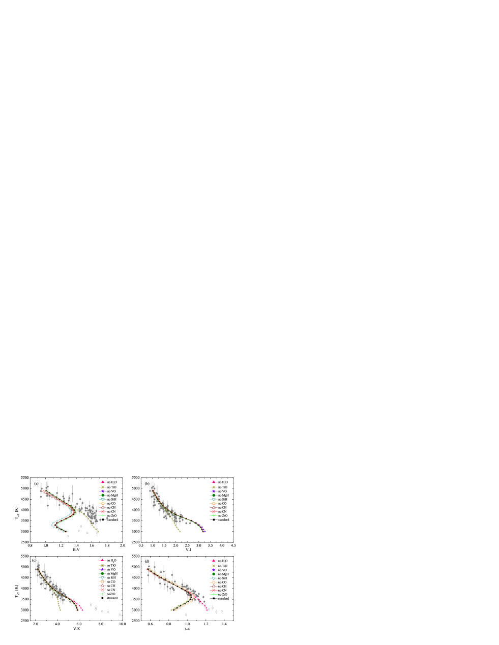
Figure 1: Influence of various molecular bands on synthetic photometric colors in different $T_{\rm eff}$–color planes (all for $\log g=3.0$). Filled circles are late-type giants from Table 3, open circles are stars from the sample of Perrin et al. (1998) (see Sect. 4 for details; stars are only plotted to indicate the spread in the observed $T_{\rm eff}$–color sequences, not for a detailed comparison). Thin lines with symbols are synthetic PHOENIX colors with certain molecules excluded from the spectral synthesis calculations. Symbols are spaced at every $100$ K.

2.3 Synthetic PHOENIX broad-band colors

The broad-band colors were calculated from synthetic spectra in the Johnson-Cousins-Glass system, using filter definitions from Bessell (1990) for the Johnson-Cousins BVRI bands and Bessell & Brett (1988) for the Johnson-Glass JHKL bands. Conversion of instrumental magnitudes to the standard Johnson-Cousins-Glass system was done using zero points derived from the synthetic colors of Vega (equating all color indices of Vega to zero). The Vega spectrum used for this purpose was calculated with the PHOENIX code employing a full NLTE treatment. Adopted atmospheric parameters were identical to those used by Castelli & Kurucz (1994): $T_{\rm eff}=9550$ K, $\log g=3.95$, metallicity $\left[\mathrm{M}/\mathrm{H}\right]=-0.5$ and microturbulent velocity $\xi=2\,\rm{km\,s^{-1}}$. Detailed Vega abundances were taken from Castelli & Kurucz (1994). Derived zero points of color indices are given in Table 1, together with those from Bessell et al. (1998). The latter were obtained using observed and theoretical color indices of Vega and Sirius, with theoretical colors computed employing the same filter transmission curves as used in this work. For the purposes of comparison, we calculated zero points using the Vega spectrum from Castelli & Kurucz (1994), which are also given in Table 1. The agreement between the three sets of zero points is generally very good. There is an indication that the PHOENIX zero points tend to be slightly larger than those of Bessell et al. (1998), though the differences are typically $\la 0.01$ mag. The discrepancies are slightly larger between the PHOENIX zero points and those calculated from the Vega spectrum of Castelli & Kurucz (1994), though they are also $\la 0.02$ mag.

The final grid of synthetic photometric colors of late type giants is given in Table 2 (available in electronic form only), and covers the following parameter space: $T_{\rm eff}=3000\dots 5000$ K (with a step of $\Delta T_{\rm eff}=100$ K), $\log g=-0.5\dots+3.5$ ($\Delta\log g=0.5$) and $\left[\mathrm{M}/\mathrm{H}\right]=+0.5\dots-4.0$ ($\Delta\left[\mathrm{M}/\mathrm{H}\right]=0.5$).

2.4 MARCS and ATLAS spectra and colors

For the comparison of synthetic colors with observations we also used colors produced with MARCS and ATLAS model atmospheres. MARCS spectra employed in this work were kindly provided to us by B. Plez (private communication, 2003). Models were calculated in the plane-parallel geometry, using the mixing length parameter $\alpha_{\rm ML}=1.5$ (for more details about the MARCS models see Plez 2003). Broad-band photometric colors were calculated using the procedure described in Sect. 2.3.

Synthetic ATLAS broad-band photometric colors were taken from Castelli & Kurucz (2003). Models were calculated under the assumption of plane-parallel geometry, using the turbulent velocity $\xi=2\,\rm{km\,s^{-1}}$ and mixing length parameter $\alpha_{\rm ML}=1.25$. Water and TiO opacities used were identical to those employed by us in the calculation of the PHOENIX grid (see Sect. 2.1).

3 The influence of astrophysical processes and model parameters on synthetic photometric colors

The thermal structure of a model atmosphere is governed a by a number of input parameters (such as stellar mass, gravity, metallicity, etc.). Indeed, all of them have a direct influence on the emerging spectrum and photometric colors. In this Section we investigate the role and possible extent of such effects, to provide a theoretical grounding for the comparisons of model predictions with observations (Sect. 5).

3.1 Effects of molecular opacities

Spectra of the late-type stars are heavily blended by various molecular lines and bands, especially at the effective temperatures below $T_{\rm eff}\sim 4000$ K (${\rm H}_{2}{\rm O}$, TiO, VO, CO, etc.). To investigate the extent of these effects we produced a number of synthetic spectra with certain molecules ‘switched off’ during the spectral synthesis calculations. In this procedure model structures were calculated as usual, i.e., employing opacities of all relevant molecules, as in the calculation of all standard spectra in the model grid discussed in Sect. 2. The spectral synthesis, however, was done subsequently for several different cases without using opacities of certain key molecules (${\rm H}_{2}{\rm O}$, TiO, VO, MgH, SiH, CO, CH, CN, and ZrO). The resulting spectra are thus different from the standard ones, as lines/bands of certain molecules are not seen in the spectra, while the physics involved in the calculations of the model structures is identical in all cases. The differences between the synthetic colors calculated from these spectra and the standard spectrum (i.e., the one with all opacities ‘on’) clearly show the effect of a particular molecule on a given photometric color (Fig. 1, $T_{\rm eff}$–color planes; Fig. 2, color–color planes).

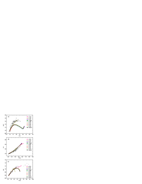
Figure 2: Same as Fig. 1 but in the color–color planes.

Obviously, TiO is by far the most influential molecule in the optical wavelength range. It is responsible for the turn-off toward the bluer color in the $T_{\rm eff}$–$(B-V)$ plane at $T_{\rm eff}\sim 3700$ K, and for the significant reddening of photometric colors below $T_{\rm eff}\sim 4000$ K in the $T_{\rm eff}$–$(V-I)$ and $T_{\rm eff}$–$(V-K)$ planes. The reddening of $V-I$ and $V-K$ colors is caused by the increasing strength of TiO lines in the $V$ band with decreasing $T_{\rm eff}$: since the $I$ band is much less influenced by TiO bands than the $V$ band (while the $K$ is not affected), $V-I$ and $V-K$ colors gradually become redder at low effective temperatures (the reason why $B-V$ gets bluer below $T_{\rm eff}\sim 3700$ K is explained in Sect. 3.2). There is also some influence of TiO on $J-K$, due to TiO lines in the $J$ band.

Water opacity is significant in all near-infrared photometric bands. Most affected is the $J-K$ color, as ${\rm H}_{2}{\rm O}$ lines are strong both in $J$ and $K$ bands. Note however that effects of ${\rm H}_{2}{\rm O}$ become noticeable only at lower effective temperatures ($T_{\rm eff}\leq 3700$ K). There is a weak influence of CO and CN on the $J-K$ color too, due to CO lines on the edges of $J$ and $K$ bands, and CN in the $J$ band (the latter comes into play only at $T_{\rm eff}\ga 4000$ K).

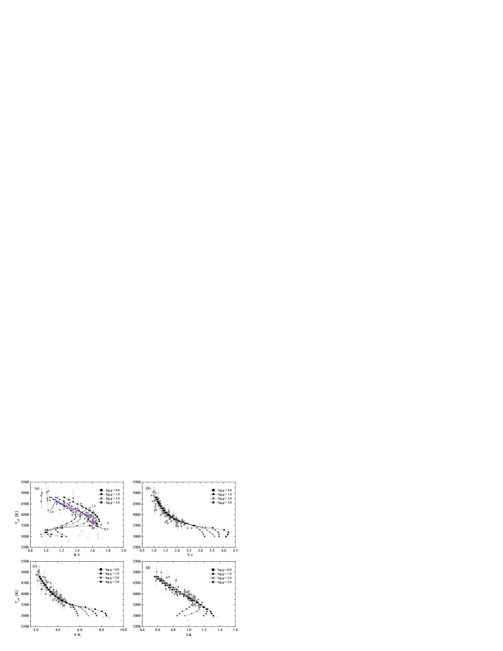
Figure 3: Influence of gravity on broad-band photometric colors in the $T_{\rm eff}$–color planes. Filled circles are late-type giants from Table 3, open circles are stars from the sample of Perrin et al. (1998) (see Sect. 4 for details; stars are only plotted to indicate the spread in the observed $T_{\rm eff}$–color sequences, not for a detailed comparison). Thin lines with symbols are the new PHOENIX colors at different $\log g$ values (symbols are spaced at every $100$ K). Thick solid line with open rectangles in panel (a) shows $T_{\rm eff}$–$\log g$–$(B-V)$ locii for the sample of late-type giants in the solar neighborhood (Sect. 4), with gravities assigned according to the $T_{\rm eff}$–$\log g$ relation of Houdashelt et al. (2000a). Numbers next to the open rectangles are $\log g$ values, with symbols plotted at every $0.5$ dex in $\log g$. Note a strong sensitivity of the $B-V$ color on $\log g$ in the entire effective temperature range.

Optical photometric colors are also noticeably affected by SiH, MgH, VO, CH, CN, and ZrO. The strongest lines of SiH and MgH are located in the blue part of the spectrum ($\sim$400–450 nm and $\sim$450–550 nm, respectively), affecting the $B$ band flux in the former case and $V$ band flux in the latter. The $B-V$ color is rather strongly influenced also by CH and to a smaller extent by CN, due to CH lines in the $B$ band (especially the G-band at $\sim 430$ nm), and CN bands both in $B$ and $V$. In both cases the effect sets in at higher temperatures ($T_{\rm eff}\ga 3800$ K). There is a weak influence of ZrO on the $B-V$ color too, due to ZrO bands at $\sim$550–700 nm. The strongest VO lines are in the wavelength range of $\sim$700–900 nm, thus mostly influencing the $I$ band.

The trends in the color–color diagrams essentially follow those in the $T_{\rm eff}$–color planes (Fig. 2). It is interesting to note that the $(V-I)$–$(V-K)$ plane is relatively little influenced by the molecular opacities (relative to the observed spread in photometric colors), even those of TiO (as both $V-I$ and $V-K$ colors get considerably bluer without TiO, the overall trend is little affected).

In general, the influence of different molecules on the broad-band photometric colors is small at $T_{\rm eff}\geq 4000$ K, except for some influence of SiH, CH ($B$ band), CN ($B$, $V$), and CO ($J$, $K$).

3.2 Effects of gravity

For a given stellar mass and effective temperature, surface gravity defines the stellar radius and thus the extension and structure of the outer photosphere, where an important fraction of the emerging spectral flux is formed. Indeed, the effects of gravity must be significant in late-type giants, especially at low $T_{\rm eff}$. The actual extent of these effects on broad-band photometric colors can be seen in Figs. 3 and 4, which show the behavior of photometric colors in various $T_{\rm eff}$–color (Fig. 3) and color–color planes (Fig. 4) at different gravities.

The influence of gravity on broad-band photometric colors is generally small above $\sim$3700 K. $V-K$ is especially robust in this sense; little sensitivity is also seen for $V-I$ and $J-K$, both in the $T_{\rm eff}$–color and color–color domains. At these relatively high temperatures, only a few molecules, e.g., H₂, CO, CH and SiH, survive at gravities between $0.0$ and $3.0$, thus having little effect on the colors. At lower temperatures, $\la 3500$ K, the gravity has a much larger effect on the chemistry of the atmosphere; for example, water vapor begins to form for $\log g=3.0$, whereas it is absent at $\log g=0.0$. Therefore, the colors are more gravity dependent at $T_{\rm eff}\sim 3500$ K than at $\sim$3700 K.

Obviously, the influence of gravity is strongest for the $B-V$ color, which is clearly reflected in the $T_{\rm eff}$–$(B-V)$ and $(B-V)$–$(V-I)$ planes (Figs. 3a, 4a). This results from the fact that the temperature structure of the atmospheres changes with the gravity: at low gravity, the atmospheres are more extended giving lower gas temperatures than at higher gravities. For example, at $T_{\rm eff}\sim 3500$ K the outermost temperature of the atmosphere models is about $2100$ K for $\log g=0.0$ whereas it is $\sim$2300 K for $\log g=3.0$. The differences in the model stratifications have a strong influence on molecule formation, which is much more efficient in the cooler, low gravity models. Since the $B-V$ color is very sensitive to molecular opacities (TiO, SiH, etc.), the influence of gravity on this color is strong.

Another feature clearly seen in the $T_{\rm eff}$–$(B-V)$ and $(B-V)$–$(V-I)$ diagrams at all gravities is a ‘turn-off’ towards the bluer colors in $B-V$ at $\sim$3700–3900 K. This inversion occurs because the $V$-band flux is strongly affected by the TiO opacity, which is growing rapidly with decreasing $T_{\rm eff}$. The TiO lines are much weaker in the $B$-band, thus the decrease of $B$-band flux is essentially governed by the shift of the maximum of the emitted spectral energy towards longer wavelengths with decreasing $T_{\rm eff}$. The net effect is that below $T_{\rm eff}\sim 4200$ K the total flux in the $V$-band decreases faster with decreasing $T_{\rm eff}$ than in the $B$-band, causing the turn-off in $B-V$ at $T_{\rm eff}\sim 3700$–$3900$ K.

Interestingly, this effect has been noticed observationally nearly four decades ago (e.g., Johnson 1966; Wing 1967). Wing (1967) has found that observed $B-V$ color of late-type giants reaches its maximum value of $B-V\simeq 1.65$ at around M2 III in $T$–$(B-V)$ plane (here $T$ is a black-body temperature measured from the black-body fit to two pseudo-continuum points in the 0.75–1.04 micron range). This corresponds to $T_{\rm eff}\simeq 3710$ K according to the effective temperature – spectral type scale of Pickles (1998). At lower temperatures, the observed $B-V$ colors stay essentially unchanged for M0 III–M4 III, then become bluer for later spectral types and finally turn to the red again for the coolest giants. It should be noted that below $T_{\rm eff}\sim 3500$ K the bluest observed $B-V$ color in the sample of Wing (1967) corresponds to $B-V\sim 1.4$, while theoretical models predict $B-V\la 1.2$. Unfortunately, the lack of knowledge of effective temperatures (or precise spectral types) for the late-type giants in the sample of Wing (1967) does not allow us to make a direct comparison of his findings with the synthetic colors calculated using current stellar atmosphere models in the $T_{\rm eff}$–$(B-V)$ plane.

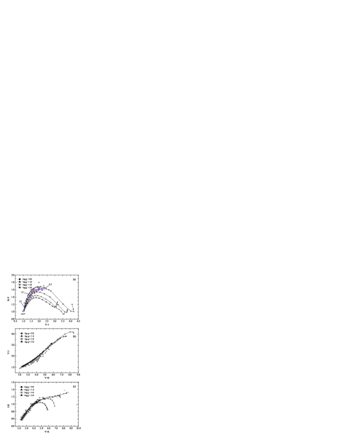
Figure 4: Same as Fig. 3 but in the color–color planes.

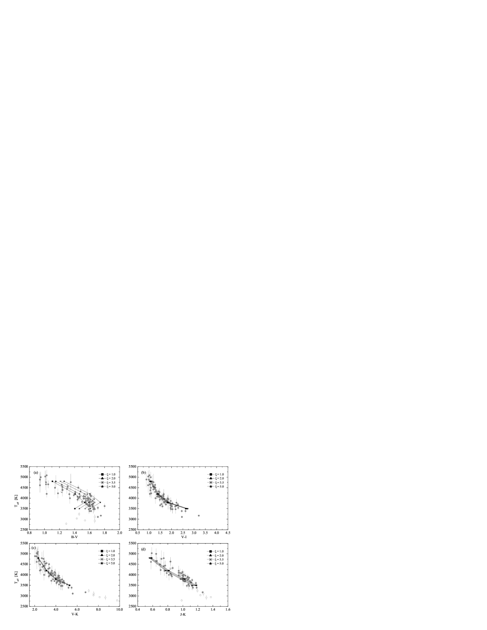
Figure 5: Influence of microturbulent velocity on synthetic photometric colors in different $T_{\rm eff}$–color planes (all for $\log g=0.5$). Filled circles are late-type giants from Table 3, open circles are stars from the sample of Perrin et al. (1998) (see Sect. 4 for details; stars are only plotted to indicate the spread in the observed $T_{\rm eff}$–color sequences, not for a detailed comparison). Thin lines with symbols are synthetic PHOENIX colors at different microturbulent velocities.

A similar effect can be seen in the mean observed $B-V$ colors of late-type giants provided by Johnson (1966), with the turn-off at around M3 III ($T_{\rm eff}\simeq 3630$ K on the scale of Pickles 1998), and with the maximum value of $B-V\simeq 1.60$. Observed colors of late-type giants in the sample of Perrin et al. (1998) show hints of this turn-off too (Fig. 3). However, in all these cases the effect seems to set in at somewhat lower effective temperatures than predicted by the theoretical models: typically, the turn-off in theoretical colors occurs at $T_{\rm eff}\sim 3700-3800$ K, while the observations point to $T_{\rm eff}\sim 3600-3700$ K (see Sect. 5 below for a detailed discussion). Note however, that stars in the sample of Perrin et al. (1998) are all variable and this may indeed influence their $B-V$ colors. This may be the case with the coolest giants in the sample of Wing (1967) too. Reconstruction of photometric colors of a ‘parent star’ (i.e., a static star with the same parameters as the variable) is not trivial in case of long-period variables (Hofmann et al. 1998), since a simple averaging of the photometric colors over the pulsational cycle is generally not appropriate. This may thus easily bias the $T_{\rm eff}$–color scales at the lower effective temperature end, i.e., below $T_{\rm eff}\la 3500$ K. It is perhaps worthwhile to note in this respect that in our search for the published interferometric effective temperatures of late-type giants in the solar neighborhood we found no non-variable giants with effective temperatures lower than $T_{\rm eff}\sim 3400$ K.

It should be stressed that all colors are significantly influenced by gravity below $T_{\rm eff}\sim 3600$ K, due to the onset of rapid molecule formation at these temperatures. The ‘turn-off’ towards bluer colors seen in all color domains at $T_{\rm eff}\la 3500$ K is thus produced by the increasing opacities of various molecules (TiO, ${\rm H}_{2}{\rm O}$, VO, etc.). The position of the ‘turn-off’ is gravity dependent, since the models with lower gravity are cooler leading to a higher rate of molecule formation.

Note however, that at these very low effective temperatures and gravities the atmospheres of late-type giants become very extended, thus stellar atmosphere models employing plane-parallel geometry (e.g., ATLAS) will be not adequate. In fact, spherical models may be insufficient too, since non-spherical and non-stationary phenomena (convection, variability, shock-waves, mass loss, etc.) will become increasingly important in this effective temperature and gravity domain (as hinted, for example, by 3D models of the red supergiant Betelgeuse, Freytag et al. 2002).

3.3 Effects of microturbulent velocity

Grids of synthetic colors produced with PHOENIX, MARCS, and ATLAS model atmospheres (Sect. 2.3) are based on the synthetic spectra calculated using a single value of microturbulent velocity, $\xi=2.0$ km s^-1. Indeed, variations around this value must be anticipated in real stars. To investigate the effect of these variations on the broad-band photometric colors we have calculated a set of PHOENIX models and spectra at several additional values of microturbulent velocity, $\xi=1.0,3.5,5.0$ km s^-1. The results are summarized in Figs. 5-6, which show the influence of $\xi$ in the $T_{\rm eff}$–color and color–color planes. Fig. 7 provides a more detailed view on the differences between colors calculated at any particular value of microturbulent velocity and those at $\xi=2.0$ km s^-1, at several effective temperatures.

Clearly, $B-V$ color is most sensitive to changes in microturbulent velocity (Fig. 5a). The differences are indeed significant, $\Delta(B-V)\sim 0.2$ mag at $T_{\rm eff}=3600$ K for colors corresponding to $\xi=1.0$ and $5.0$ km s^-1. The flux in the $B$ and $V$ band is affected by changes in $\xi$ (though the effect is considerably stronger in the $B$ band), and in both cases the flux is lower at higher microturbulent velocities, mostly due to the increasing line blending with higher $\xi$. The effect is smaller but still non-negligible in case of $V-I$ and $J-K$ (up to $\sim 0.1$ mag, Figs. 5b-c). The only color that is essentially unaffected by the changes in microturbulent velocity is $V-K$ (Fig. 5d). In this case the flux in $V$ and $K$ bands is lower at higher values of $\xi$ by a comparable amount (mostly due to increasing line widths of numerous atomic lines in the former case and due to changes in the width of CO bands in the latter), thus the $V-K$ color remains essentially unaffected.

In general, differences between colors corresponding to different $\xi$ are largest at lower effective temperatures but they remain significant even at relatively high temperatures, e.g., $T_{\rm eff}\ga 4500$ K. The effect of microturbulent velocity is somewhat smaller at higher gravities, which is related to the fact that at higher $\log g$ spectral lines are broader than at lower gravities and thus the relative broadening due to the increasing microturbulent velocity (or vice versa) is smaller. Hence, the emitted flux and thus the photometric colors are affected less than at lower gravities.

Trends in the color–color diagrams follow those seen in the $T_{\rm eff}$–color planes. The effect is largest in the $(B-V)$–$(V-I)$ plane, especially at lowest effective temperatures, due to the sensitivity of the $B-V$ color to changes in the microturbulent velocity. The effect is also significant in the $(J-K)$–$(V-K)$ plane where differences in the $J-K$ color are comparable with the spread in the observed giant sequence. The $(V-I)$–$(V-K)$ plane is little affected since the influence of $\xi$ is small both in the case of the $(V-I)$ and $(V-K)$ color.

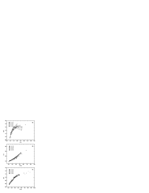
Figure 6: Same as Fig. 5 but in the color–color planes.

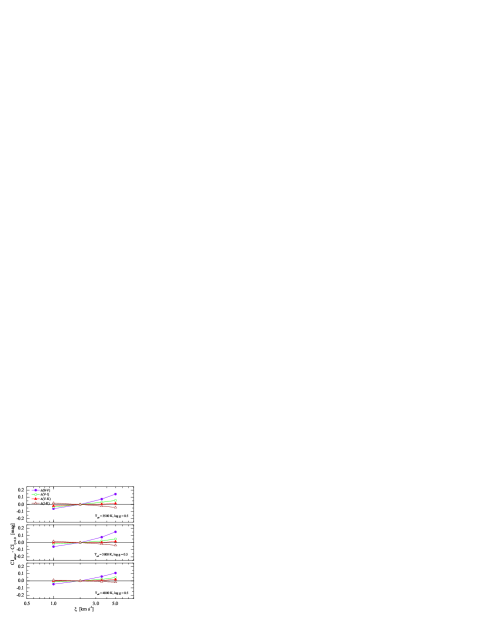
Figure 7: Effect of microturbulent velocity ($\xi$) on broad-band photometric colors at different effective temperatures (the ordinate is the difference between the photometric color index for a given microturbulent velocity and that for $\xi=2.0$ km ${\rm s^{-1}}$).

3.4 Effects of stellar mass

The influence of stellar mass on broad-band colors is illustrated in Fig. 8, where we plot differences between the photometric colors corresponding to stars of different masses (${\rm CI(M_{\star})}-{\rm CI(M_{\star}=M_{\odot})}$) at several effective temperatures, for $\log g=0.5$ (the differences are smaller at higher gravities). The effect of stellar mass is most pronounced at lower effective temperatures ($T_{\rm eff}\la 4500$ K), where differences in e.g. $V-K$ may reach $\sim$0.1 mag at $T_{\rm eff}\sim 3500$ K when comparing stars with $M_{\star}=1.0$ and $5.0\,M_{\odot}$. The effect becomes smaller at higher effective temperatures, but is for some colors non-negligible even at $T_{\rm eff}\sim 4800$ K (Fig. 8).

It should be noted, however, that these differences do not simply mimic the effect of gravity. It has been shown above that, for instance, $B-V$ is rather sensitive to gravity, while $V-K$ remains essentially unaffected. The situation is opposite in terms of sensitivity to stellar mass (Fig. 8), which shows that stellar interiors respond in a rather different way to changes in mass and gravity. To a large extent this is determined by the fact that the atmospheric structure essentially remains unaltered with changing stellar mass (on the scale of optical depth), though the outer layers are marginally hotter for $M_{\star}=5M_{\odot}$ than $1M_{\odot}$ (especially at lower effective temperatures). Together with changes in the molecular dissociation equilibria, this produces a slight shift of the photometric colors towards the higher effective temperatures seen in Fig. 8. Since PHOENIX spectra and colors are calculated for the stellar mass of $M_{\star}=1M_{\odot}$, these effects should be taken into account when using them with stars of considerably different masses.

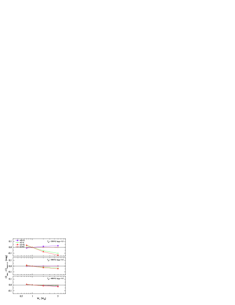
Figure 8: Effect of stellar mass on broad-band photometric colors at different effective temperatures (the ordinate is the difference between the photometric color index for a given stellar mass and that for $M_{\star}=1.0$ ${\rm M}_{\odot}$).

3.5 Influence of the treatment of convection

The new grid of PHOENIX spectra/colors presented in this work employs a mixing length parameter $\alpha_{\rm ML}=2.0$ which was motivated by results from the 3D hydrodynamic modeling of M-type pre-main sequence objects and dwarf stars (Ludwig 2003). All 1D standard model atmospheres of evolved giants discussed so far in this paper predict that the structure of the optically thin layers hardly depends on the assumed mixing length parameter: we find that relative differences in the spectral flux for the PHOENIX models calculated with the mixing lengths of $\alpha_{\rm ML}=1.5$ and $2.0$ are small (typically of the order of few tenths of a percent). Differences in the broad-band colors are very small too, typically within a few milimagnitudes. The situation with MARCS spectra and colors is quantitatively very similar (B. Plez, private communication).

The simple reason for the insensitivity is that in the framework of mixing length theory the convective zone is confined to optically thick regions. However, the geometric distance between the upper boundary of the formally convectively unstable region (according to the Schwarzschild criterion) and optical depth unity is not large. One might speculate that in a real star convection may overshoot into the optically thin layers and thus may influence the emergent spectrum.

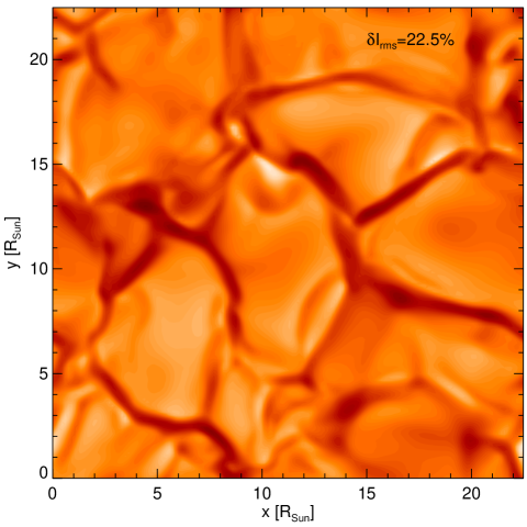
Figure 9: Snapshot of the emergent white light intensity during the temporal evolution of a hydrodynamical red giant model. Note the presence of the granulation pattern, and its spatial scales. The relative root-mean-squares contrast of the intensity amounts to 22.5 % at this particular instant in time.

To test the idea we performed an exploratory study, and constructed a 3-dimensional hydrodynamical model atmosphere for a prototypical late-type giant with $T_{\rm eff}\simeq 3700$ K, $\log g=1.0$, and ${\rm\left[\mathrm{M}/\mathrm{H}\right]}=0.0$. For this purpose we employed the radiation-hydrodynamics code CO⁵BOLD mainly developed by B. Freytag and M. Steffen; for a description of the code see Wedemeyer et al. (2004). The model is a so-called ‘local box’ model employing grey radiative transfer and Cartesian geometry. The computational box contains the optically thin atmosphere and the upper part of the optically thick convective stellar envelope. Details of the model will be discussed elsewhere (Ludwig et al. 2005, in preparation), while in this study we concentrate on issues related to spectral properties. Figure 9 shows a snapshot of the emergent intensity during the temporal evolution of the model. One immediately realizes the presence of a granulation pattern. Similar to 1D hydrostatic model atmospheres based on mixing length theory the average vertical structure of the hydrodynamical model is such that the stratification becomes formally convectively stable already in optically thick layers. Hence, the granular pattern is a consequence of intense convective overshooting. The time-averaged relative root-mean-squares intensity contrast amounts to $22.5$ %, which is larger than the contrast of solar granulation ($18$ % white light contrast).

To obtain an estimate of the amount of the color changes due to convection-related effects we performed spectral synthesis calculations for the hydrodynamical model atmosphere, and compared them to corresponding results from a standard 1D hydrostatic model atmosphere based on mixing length theory but otherwise identical input physics. In particular, we used the same equation of state and grey PHOENIX opacities in the hydrodynamical and hydrostatic model. Turbulent pressure was neglected when solving the hydrostatic equation. In the hydrodynamical model turbulent pressure makes a substantial contribution to the dynamical balance. It leads to a lifting of the optically thin layers to larger radii, and also alters to some extent their pressure-temperature relation. The neglect of turbulent pressure in the 1D model has nevertheless no consequences for our comparison. Due to the confinement of convection to the optically thick layers no reasonable choice of the treatment of turbulent pressure in the 1D model alters the pressure-temperature relation of the optically thin layers, or might allow to emulate the behavior of the hydrodynamical model.

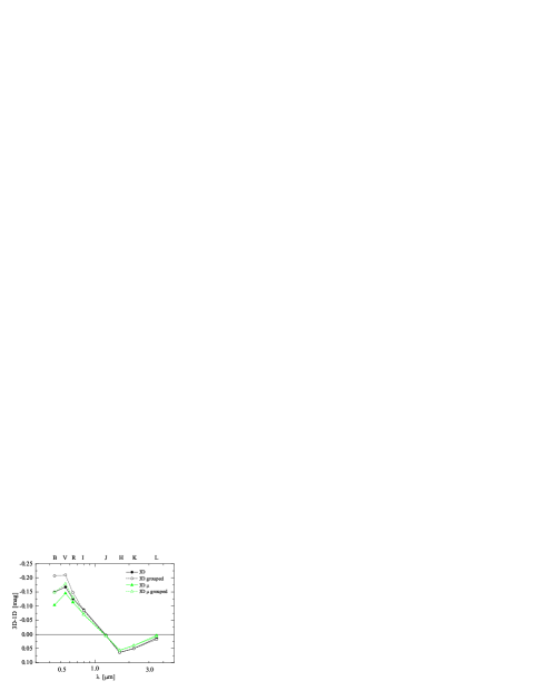
Figure 10: Influence of surface granulation on the broad-band photometric colors of the prototypical red giant, as reflected by magnitude differences in various band-passes (indicated on the top of the panel) between the predictions of 3D hydrodynamical and classical 1D model atmospheres. See text for details.

Because of time stepping constraints related to short radiative time scales the calculation of the hydrodynamical giant model was very time consuming. We were only able to gather data of a rather short time sequence limiting the obtainable statistical accuracy. The hydrodynamical spatio-temporal model has $150\times 150\times 100$ grid points ($X\times Y\times Z$, where $Z$ is vertical), which corresponds to $15750\times 15750\times 8602$ ${\rm Mm}^{3}$ geometrical box size, and provides a total of $2.25\times 10^{6}$ pressure-temperature profiles. Together with the typical number of $\sim 5\times 10^{5}$ wavelength points usually used in the framework of PHOENIX it renders the spectral synthesis problem intractable if one tries to calculate spectra for all thermal profiles individually, and subsequently averages them to obtain the observable spectrum. Instead, we used an approximate approach and sorted the individual thermal profiles into nine groups of increasing emergent white light intensity. This corresponds in Fig. 9 to a sorting of points depending on whether they belong to an inter-granular lane or increasingly brighter parts of a granule. This classification turns out to group together thermally as well kinematically (in terms of velocity) similar vertical stratifications. The stratifications associated with a particular group were then averaged on surfaces of equal optical depth. The resulting nine stratifications were treated as standard 1D model atmospheres for which spectral synthesis calculations were performed. The nine radiation fields were added weighted by their respective surface area fraction. For the further comparison we also obtained a ‘global average’, by averaging over all pressure-temperature profiles.

Figure 10 shows resulting flux ratios (expressed as magnitude differences) between the 3D hydrodynamical and 1D hydrostatic models integrated over various band-passes. We corrected small mismatches in total flux of the individual synthetic spectra by scaling them with a wavelength independent factor to obtain the same nominal flux. The representation of fluxes in Fig. 10 also allows to calculate color differences 3D$-$1D by simply subtracting the magnitudes in corresponding filters. The global average (‘3D’) contains effects on the radiation field merely associated with the different vertical structure of the hydrodynamical atmosphere, while the superposition of the radiation fields of the individual 9 groups contains additional effects related to thermal inhomogeneities in horizontal directions (‘3D grouped’). Consequently, differences 3D$-$1D become somewhat larger in the ‘grouped’ case. They are most pronounced towards shorter wavelength due to the more strongly non-linear dependence of the source function on temperature so that horizontal temperature inhomogeneities can more easily leave a noticeable imprint in the average emergent radiation field.

Obviously, the grouping procedure described before ignores the geometry of the flow for off-center positions on the stellar disk. Each horizontal position is represented by a plane-parallel infinitely extended model atmosphere, ignoring the neighborhood of hot and cool areas. To include more accurately the 3D effects of the center-to-limb variation we extended our classification scheme by keeping the groups but calculated the average structures and radiation fields for inclined viewing angles (three in total) separately, including the full information about the flow geometry. Figure 10 shows that the 3D limb effects tend to decrease the deviations 3D$-$1D. The lines ‘3D’ and ‘3D $\mu$’ (for the case of including 3D limb effects) depict the case where horizontal fluctuations are not explicitly accounted for. Lines-of-sight at inclined viewing angles pass through parts of the atmosphere belonging to different groups, thus leading to some ‘mixing’ between the groups which should reduce the effects of horizontal fluctuations. Indeed, the inclusion of horizontal fluctuations lead to slightly more pronounced differences as depicted by the lines ‘3D grouped’ (3D limb effects ignored but horizontal fluctuations included) and ‘3D $\mu$ grouped’ (3D limb effects and horizontal fluctuations included). However, all approaches provide a rather similar picture indicating that the difference in the mean vertical structure of 3D and 1D model is the dominant factor for the differences in the band-integrated fluxes (resp. colors).

The flux differences 3D$-$1D may lead to noticeable differences in effective temperatures when they are derived from photometric colors based on 1D standard model atmospheres (e.g., the difference in $(V-K)$ of $\sim$0.2 translates to an offset in $T_{\rm eff}$ by $\sim 70$ K). However, the changes in $T_{\rm eff}$ and photometric colors are too small to alter significantly the correspondence between theoretical and empirical colors as well as temperatures discussed in Sect. 5. Nevertheless, our calculations provide an estimate of the intrinsic limitation of 1D hydrostatic model atmospheres in reproducing the radiative properties of evolved late-type giants.

In convective stellar atmosphere models one often encounters the situation that the temperature gradient in the continuum forming layers depends to some extent on the mixing length parameter. This has the consequence that predicted stellar colors depend on this parameter which also allows to offset mismatches to observed colors by choosing a suitable value (e.g., Heiter et al. 2002). As stated before, due to the insensitivity to the mixing length parameter, this possibility does not exist in the case of late-type giants. In principle, this makes them interesting test cases for convection theories. However, due to uncertainties in our knowledge of other physical properties of their atmospheres – in particular opacities – such tests are somewhat hampered in practice.

Table 3: A sample of late-type giants in the solar neighborhood with precise interferometric derivations of $T_{\rm eff}$ from the literature. Photometric colors are given in Johnson-Cousins-Glass system (see Sect. 4 for details). References for spectral types, angular diameters, effective temperatures: 1. van Belle et al. (1999); 2. Perrin et al. (1998); 3. Dyck et al. (1998); 4. Dyck et al. (1996); 5. Di Benedetto (1993); 6. Ridgway et al. (1980). References for photometry: 10. SIMBAD; 11. Neugebauer & Leighton (1969); 12. Borde et al. (2002); 13. Gezari et al. (1999); 14. Morel & Magnenat (1978); 15. Ducati (2002).

HD	HR	Other	Sp type	$\theta_{\rm R}$		$T_{\rm eff}$		Ref	$V$	$B\!-\!V$	$V\!-\!I$	$V\!-\!K$	$J\!-\!K$	Ref
				mas		K
1632	79		K5 III	$2.51$$\,\pm\,$	$0.05$	$3844$$\,\pm\,$	$90$	1	5.79	1.60	2.13	3.98	0.99	10, 11, 12
5316	259		M4 III	$3.67$$\,\pm\,$	$0.10$	$3388$$\,\pm\,$	$70$	1	6.23	1.62	3.21	5.19	1.18	10, 11, 13
5820	284	WW Psc	M2.4 III	$3.16$$\,\pm\,$	$0.16$	$3480$$\,\pm\,$	$90$	6	6.11	1.67	1.97	4.53	1.05	10, 14
6860	337	$\beta$ And	M0+IIIa	$12.5$$\,\pm\,$	$0.6$	$4002$$\,\pm\,$	$178$	3	2.05	1.57	1.76	3.87	1.01	10, 14
			M0 III	$14.35$$\,\pm\,$	$0.19$	$3705$$\,\pm\,$	$45$	5
7087	351	$\chi$ Psc	G8.5 III	$1.64$$\,\pm\,$	$0.07$	$5087$$\,\pm\,$	$256$	1	4.66	1.03	1.30	2.30	–	10, 14
8126	389	91 Psc	K5 III	$2.22$$\,\pm\,$	$0.06$	$4144$$\,\pm\,$	$108$	1	5.23	1.39	1.80	3.29	–	10, 11
9640	450		M2 III	$2.42$$\,\pm\,$	$0.05$	$3825$$\,\pm\,$	$96$	1	5.91	1.50	2.18	4.04	–	10, 11
11928	564		M2 III	$2.96$$\,\pm\,$	$0.06$	$3656$$\,\pm\,$	$72$	1	5.83	1.58	2.49	4.38	–	10, 11, 13
12929	617	$\alpha$ Ari	K2–IIIab	$6.0$$\,\pm\,$	$0.6$	$4790$$\,\pm\,$	$298$	3	2.01	1.15	1.16	2.66	0.75	12, 14
13325	631	15 Ari, AV Ari	M3 III	$3.75$$\,\pm\,$	$0.11$	$3605$$\,\pm\,$	$84$	1	5.70	1.64	2.78	4.77	1.17	10, 11, 13
15656	736	14 Tri	K5 III	$2.60$$\,\pm\,$	$0.11$	$4057$$\,\pm\,$	$124$	1	5.16	1.47	1.87	3.52	0.84	10, 11, 12
18449	882	24 Per	K2 III	$2.08$$\,\pm\,$	$0.07$	$4416$$\,\pm\,$	$192$	1	4.93	1.24	1.52	2.83	0.75	10, 12
18884	911	$\alpha$ Cet	M1.5 IIIa	$11.9$$\,\pm\,$	$0.4$	$3869$$\,\pm\,$	$161$	3	2.53	1.64	1.97	4.16	1.06	10, 14
27348	1343	54 Per	G8 III	$1.44$$\,\pm\,$	$0.13$	$4878$$\,\pm\,$	$290$	1	4.93	0.94	1.27	2.17	–	10, 11
28305	1409	$\epsilon$ Tau	G9.5 III	$2.57$$\,\pm\,$	$0.06$	$5027$$\,\pm\,$	$280$	1	3.54	1.01	1.23	2.19	0.59	10, 14
29139	1457	$\alpha$ Tau	K5 III	$20.44$$\,\pm\,$	$0.11$	$3947$$\,\pm\,$	$41$	2	0.86	1.54	1.70	3.66	0.97	10, 14
				$20.21$$\,\pm\,$	$0.30$	$3970$$\,\pm\,$	$49$	5
30504	1533	1 Aur	K3.5 III	$2.93$$\,\pm\,$	$0.08$	$4067$$\,\pm\,$	$111$	1	4.89	1.44	1.81	3.63	–	10, 11, 13
30834	1551	2 Aur	K2.5 III	$2.79$$\,\pm\,$	$0.06$	$4290$$\,\pm\,$	$183$	1	4.77	1.41	1.87	3.28	–	10
33463		NSV16257	M2 III?	$2.87$$\,\pm\,$	$0.06$	$3623$$\,\pm\,$	$122$	1	6.40	1.80	2.54	4.79	–	10, 11
34559	1739	109 Tau	G8 III	$1.42$$\,\pm\,$	$0.13$	$4887$$\,\pm\,$	$362$	1	4.92	0.94	1.13	2.03	–	10, 11
38656	1995	$\tau$ Aur	G8 III	$1.97$$\,\pm\,$	$0.08$	$4616$$\,\pm\,$	$344$	1	4.53	0.94	1.22	2.19	0.58	10
39003	2012	$\nu$ Aur	K0 III	$2.79$$\,\pm\,$	$0.06$	$4496$$\,\pm\,$	$329$	1	3.97	1.14	1.38	2.52	0.70	10, 12
42471	2189		M2 III	$2.94$$\,\pm\,$	$0.06$	$3954$$\,\pm\,$	$205$	1	5.78	1.66	2.38	4.29	–	10, 11
43039	2219	$\kappa$ Aur	G9 III	$2.16$$\,\pm\,$	$0.09$	$4660$$\,\pm\,$	$276$	1	4.34	1.02	1.33	2.40	0.65	10
54716	2696	63 Aur	K3.5 III	$2.92$$\,\pm\,$	$0.10$	$3995$$\,\pm\,$	$110$	1	4.94	1.45	1.99	3.42	0.85	10, 11, 12
57669	2805	66 Aur	K1 III	$1.94$$\,\pm\,$	$0.17$	$4375$$\,\pm\,$	$289$	1	5.22	1.24	1.35	2.72	–	10, 11
61338	2938	74 Gem, NSV3671	M0.0 III	$2.97$$\,\pm\,$	$0.29$	$4090$$\,\pm\,$	$200$	6	5.05	1.62	1.64	3.94	0.97	11, 12
78712	3639	RS Cnc	M6.9 III	$14.77$$\,\pm\,$	$0.09$	$3110$$\,\pm\,$	$117$	2	5.95	1.67	–	7.56	1.27	10, 14
80493	3705	$\alpha$ Lyn	K7 IIIab	$7.4$$\,\pm\,$	$0.6$	$3969$$\,\pm\,$	$220$	3	3.13	1.55	1.67	3.73	1.00	10, 14
			K7 III	$7.98$$\,\pm\,$	$0.31$	$3791$$\,\pm\,$	$82$	5
86663	3950	$\pi$ Leo, NSV4699	M1.7 IIIab	$4.88$$\,\pm\,$	$0.28$	$3710$$\,\pm\,$	$110$	6	4.70	1.60	1.97	4.18	1.03	13, 14
87837	3980	31 Leo	K4.2 III	$3.55$$\,\pm\,$	$0.22$	$3930$$\,\pm\,$	$120$	6	4.38	1.44	1.48	3.33	0.86	12, 13, 14
99998	4432	87 Leo	K4.5 III	$3.71$$\,\pm\,$	$0.35$	$3720$$\,\pm\,$	$170$	6	4.77	1.56	1.55	3.57	1.00	11, 12
108849		BK Vir	M7.4 III	$11.11$$\,\pm\,$	$0.23$	$2944$$\,\pm\,$	$34$	2	7.28	1.54	–	8.12	1.37	10, 11, 13
112300	4910	$\delta$ Vir	M3+III	$10.0$$\,\pm\,$	$0.6$	$3783$$\,\pm\,$	$182$	3	3.38	1.59	2.22	4.59	1.07	10, 14
114961		SW Vir	M8 III	$17.40$$\,\pm\,$	$0.12$	$2921$$\,\pm\,$	$110$	2	6.85	1.67	–	8.65	1.31	10, 11, 13, 15
119149	5150	82 Vir	M2.1 IIIa	$4.34$$\,\pm\,$	$0.25$	$3690$$\,\pm\,$	$110$	6	5.01	1.63	1.98	4.33	1.02	11, 13, 15
120819	5215	NSV6468	M2 III	$2.50$$\,\pm\,$	$0.05$	$3823$$\,\pm\,$	$83$	1	5.87	1.62	2.20	4.18	1.04	11, 15
124897	5340	$\alpha$ Boo	K1.5 III	$20.91$$\,\pm\,$	$0.08$	$4321$$\,\pm\,$	$44$	2	–0.05	1.23	1.27	2.91	0.84	10, 14
				$19.5$$\,\pm\,$	$1.0$	$4628$$\,\pm\,$	$210$	3
				$19.5$$\,\pm\,$	$1.0$	$4628$$\,\pm\,$	$133$	4
			K1 III	$20.95$$\,\pm\,$	$0.2$	$4294$$\,\pm\,$	$30$	5
126327		RX Boo	M8 III	$18.87$$\,\pm\,$	$0.12$	$2786$$\,\pm\,$	$46$	2	7.96	1.29	–	9.76	0.99	10, 11, 13
127665	5429	$\rho$ Aur, NSV6697	K3 III	$3.80$$\,\pm\,$	$0.12$	$4440$$\,\pm\,$	$228$	1	3.59	1.30	–	2.94	0.77	10, 12
130084	5510		M1 III	$2.07$$\,\pm\,$	$0.05$	$3962$$\,\pm\,$	$108$	1	6.26	1.58	2.10	4.21	1.03	10, 11
131873	5563	$\beta$ UMi, NSV6846	K4–III	$9.9$$\,\pm\,$	$0.8$	$4086$$\,\pm\,$	$225$	3	2.08	1.47	1.47	3.31	0.79	10, 14
133774	5622	$\nu$ Lib	K4.8 III	$2.85$$\,\pm\,$	$0.41$	$3930$$\,\pm\,$	$270$	6	5.20	1.61	1.60	3.72	1.00	11, 12
134320	5638	46 Boo	K2 III	$1.44$$\,\pm\,$	$0.06$	$4532$$\,\pm\,$	$135$	1	5.68	1.24	1.58	3.00	–	10
135722	5681	$\delta$ Boo, NSV7002	G8 III	$2.71$$\,\pm\,$	$0.06$	$4994$$\,\pm\,$	$257$	1	3.49	0.95	1.37	2.27	0.65	10, 14
136512	5709	$o$ CrB, NSV7032	K0 III	$1.18$$\,\pm\,$	$0.07$	$4757$$\,\pm\,$	$265$	1	5.50	1.02	–	2.37	–	10
137853	5745	NSV20317	M1 III	$2.42$$\,\pm\,$	$0.05$	$3833$$\,\pm\,$	$85$	1	6.04	1.60	2.20	4.20	1.01	10, 11, 13
139216		$\tau^{4}$ Ser	M7.4 III	$11.60$$\,\pm\,$	$0.18$	$3034$$\,\pm\,$	$30$	2	6.53	1.43	–	7.53	1.23	10, 11, 13
139663	5824	42 Lib	K3 III:	$2.44$$\,\pm\,$	$0.33$	$4000$$\,\pm\,$	$260$	6	4.96	1.34	1.29	2.88	0.82	12, 14
146051	6056	$\delta$ Oph, NSV7556	M0.5 III	$10.43$$\,\pm\,$	$0.48$	$3779$$\,\pm\,$	$96$	2	2.75	1.59	1.82	3.94	1.00	10, 14
				$9.5$$\,\pm\,$	$0.4$	$3987$$\,\pm\,$	$168$	3
				$9.5$$\,\pm\,$	$0.5$	$3983$$\,\pm\,$	$117$	4
147749	6107	$\nu^{1}$ CrB, NSV7676	M2 III	$3.68$$\,\pm\,$	$0.10$	$3764$$\,\pm\,$	$136$	1	5.20	1.60	2.45	4.33	1.06	10, 11, 13
150580	6208		K3	$1.24$$\,\pm\,$	$0.06$	$4555$$\,\pm\,$	$139$	1	6.07	1.31	1.50	3.12	–	10, 11
152173	6258	50 Her, NSV20792	M1 III	$2.32$$\,\pm\,$	$0.06$	$4134$$\,\pm\,$	$124$	1	5.72	1.61	2.09	3.89	1.00	10, 11, 13, 15
160677	6584		M2 III	$2.26$$\,\pm\,$	$0.05$	$3911$$\,\pm\,$	$76$	1	6.06	1.58	2.28	4.22	1.06	10, 11, 13, 15
164058	6705	$\gamma$ Dra	K5 III	$9.8$$\,\pm\,$	$0.3$	$4095$$\,\pm\,$	$163$	3	2.22	1.52	1.55	3.55	0.95	10, 14
				$9.8$$\,\pm\,$	$0.3$	$4099$$\,\pm\,$	$80$	4
				$10.13$$\,\pm\,$	$0.24$	$3981$$\,\pm\,$	$62$	5
167193	6820		K4 III	$1.54$$\,\pm\,$	$0.06$	$4080$$\,\pm\,$	$99$	1	6.12	1.47	1.73	3.48	–	10, 11
169916	6913	$\lambda$ Sgr	K2 III:	$4.29$$\,\pm\,$	$0.33$	$4660$$\,\pm\,$	$180$	6	2.82	1.05	1.04	2.41	0.66	12, 14
175775	7150	$\xi^{2}$ Sgr	K1 III:	$3.79$$\,\pm\,$	$0.41$	$4230$$\,\pm\,$	$230$	6	3.52	1.18	1.10	2.57	0.71	12, 14
177808	7237		M0 III	$2.27$$\,\pm\,$	$0.05$	$4075$$\,\pm\,$	$86$	1	5.56	1.54	1.92	3.73	0.99	10, 11, 12, 13
177809	7238	NSV24682	M2.5 III	$2.40$$\,\pm\,$	$0.05$	$3859$$\,\pm\,$	$78$	1	6.06	1.55	2.33	4.33	1.08	10, 11, 13, 15
189319	7635	$\gamma$ Sge, NSV12638	M0–III	$5.6$$\,\pm\,$	$0.5$	$4189$$\,\pm\,$	$238$	3	3.47	1.57	1.66	3.62	0.95	10, 14
194317	7806	39 Cyg	K2.5 III	$2.99$$\,\pm\,$	$0.08$	$4192$$\,\pm\,$	$239$	1	4.44	1.33	1.72	2.99	0.76	10, 13
196610	7886	EU Del	M6 III	$11.02$$\,\pm\,$	$0.25$	$3243$$\,\pm\,$	$79$	2	6.05	1.46	–	7.09	1.19	10, 11, 13

Table 3: Continued.

HD	HR	Other	Sp type	$\theta_{\rm R}$		$T_{\rm eff}$		Ref	$V$	$B\!-\!V$	$V\!-\!I$	$V\!-\!K$	$J\!-\!K$	Ref
				mas		K
196777	7900	$\upsilon$ Cap, NSV25208	M2.1 III	$4.72$$\,\pm\,$	$0.52$	$3540$$\,\pm\,$	$190$	6	5.10	1.66	1.96	4.29	1.07	11, 13, 15
199169	8008	32 Vul, NSV13398	K4 III	$2.46$$\,\pm\,$	$0.05$	$4324$$\,\pm\,$	$113$	1	5.01	1.48	1.82	3.40	0.87	10, 11, 13, 15
200044	8044	NSV13454	M3 III	$3.33$$\,\pm\,$	$0.08$	$3615$$\,\pm\,$	$77$	1	5.65	1.61	2.58	4.42	–	10, 11
212988	8555		K3	$1.52$$\,\pm\,$	$0.06$	$4507$$\,\pm\,$	$123$	1	5.98	1.45	1.64	3.35	–	10, 11
216386	8698	$\lambda$ Aqr	M2.5 III	$9.1$$\,\pm\,$	$0.7$	$3477$$\,\pm\,$	$187$	3	3.79	1.65	2.04	4.47	1.12	10, 14
				$9.1$$\,\pm\,$	$1.0$	$3477$$\,\pm\,$	$200$	4
			M2.0 IIIa	$8.21$$\,\pm\,$	$0.44$	$3750$$\,\pm\,$	$100$	6
219215	8834	$\phi$ Aqr, NSV26044	M1.5 III	$5.44$$\,\pm\,$	$0.89$	$3770$$\,\pm\,$	$300$	6	4.22	1.55	1.85	4.03	1.00	14
221345	8930	14 And	K0 III	$1.79$$\,\pm\,$	$0.07$	$4206$$\,\pm\,$	$165$	1	5.22	1.03	1.32	2.49	–	10, 11
221662	8942	NSV26103	M3 III	$3.70$$\,\pm\,$	$0.10$	$3542$$\,\pm\,$	$103$	1	6.06	1.71	2.97	5.05	–	10, 11
223755	9035		M2.5 III	$2.46$$\,\pm\,$	$0.05$	$3660$$\,\pm\,$	$88$	1	6.12	1.60	1.93	4.09	–	10, 11
224303	9055	NSV26170	M2 III	$2.41$$\,\pm\,$	$0.05$	$3704$$\,\pm\,$	$80$	1	6.16	1.60	2.22	4.18	–	10, 11
224427	9064	$\psi$ Peg, NSV14777	M3 III	$6.5$$\,\pm\,$	$0.6$	$3475$$\,\pm\,$	$206$	3	4.66	1.59	2.18	4.61	1.08	10, 14

4 Synthetic colors versus observations: sample of late-type giants for the comparisons

4.1 Selection criteria and stellar sample

In order to make a meaningful comparison of the calculated synthetic colors with observations, a sample of stars is required for which precise basic stellar parameters (effective temperature, metallicity, gravity) are known. Ideally, such a sample should span the entire parameter range in $T_{\rm eff}$, $\log g$, $\left[\mathrm{M}/\mathrm{H}\right]$ covered by the grid of synthetic colors and should be complemented with reliable estimates of interstellar extinction for individual stars. Unfortunately, this is very difficult to achieve in practice.

A direct estimate of $T_{\rm eff}$ is possible if the angular diameter of a star is known (from interferometric measurements or lunar occultations, for instance). Recent advances in stellar interferometry and the increasing number of interferometric setups operating at optical (Mark III, NPOI) and near-infrared (IOTA, PTI) wavelengths, together with observations of lunar occultations, now allow the determination of precise angular diameters and effective temperatures for a number of late-type giants in the solar neighborhood (e.g., Richichi & Percheron 2002). Since these stars are bright, they are generally well observed, with a wealth of supplementary photometric and spectroscopic data readily available, and could therefore form the basis for a sample to be used for the purposes of this study.

A sample of late-type giants was thus selected according to the following criteria: (i) the star is a normal giant of spectral class G, K or M (no chemically or otherwise peculiar stars are included); (ii) interferometrically derived $T_{\rm eff}$ is available from the literature ($T_{\rm eff}\leq 5000$ K); (iii) the precision of the derived $T_{\rm eff}$ is better than $8\%$ (note that the accuracy is in general significantly better – see below); (iv) the star is not variable, or the amplitude of variability is less than $\Delta V\sim 0.1$. A search through the literature resulted in 56 objects matching these criteria.

Additionally, we included non-variable late-type giants from a sample of Ridgway et al. (1980; R80), for which effective temperatures were derived from lunar occultations. Historically, the R80 effective temperature scale was an important step towards a homogeneous $T_{\rm eff}$–$(V-K)$ relation for cool stars based on precise measurements of angular diameters, and it has been extensively used ever since.

We also included all stars from Perrin et al. (1998; P98), to illustrate the behavior of $T_{\rm eff}$–color relations at low effective temperatures. Though these are all variable stars, the $T_{\rm eff}$–color scale of P98 is the only available which extends to effective temperatures as low as $T_{\rm eff}\sim 2800$ K. Data from this sample were not used for the derivation of $T_{\rm eff}$–$\log g$–color scales, though.

The final sample consists of 74 nearby late-type giants with precisely derived $T_{\rm eff}$, either from interferometry (Di Benedetto 1993 (DB93); Dyck et al. 1996 (D96), 1998 (D98); P98, van Belle et al. 1999 (VB99)), or lunar occultations (R80). All stars are listed in Table 3, along with their angular diameters (Rosseland diameters, see Sect. 4.5) and effective temperatures. The median value of the (reported) error in $T_{\rm eff}$ for the sample stars is $\pm 140$ K ($\sim$3.5%); only 7 measurements have errors larger than $6\%$, while for 53 stars they are less than $5\%$.

4.2 Broad-band photometric colors

Broad-band BVIJK photometric colors of stars in Table 3 were collected from published data using the SIMBAD database. For the majority of stars data from multiple bibliographical sources were available, thus averaged colors were used in such cases (68 objects). Apart from a slight inconsistency in $I$-band colors (see below), colors extracted from different sources agree well, typically to within $\sim$0.04 mag or better.

$I$-band photometry was extracted from the SIMBAD database (Johnson $I$), and/or the Two-Micron Sky Survey (TMSS) catalog of Neugebauer & Leighton (1969); 20 objects had $I$-band observations in both systems, while none had photometry in Cousins $I$. The $V-I$ colors were transformed to the Johnson-Cousins-Glass system using relations from Fernie (1983) for Johnson $(V-I)_{\rm J}$ and from Bessell & Weis (1987) for $(V-I)_{\rm TMSS}$ from the TMSS catalog.

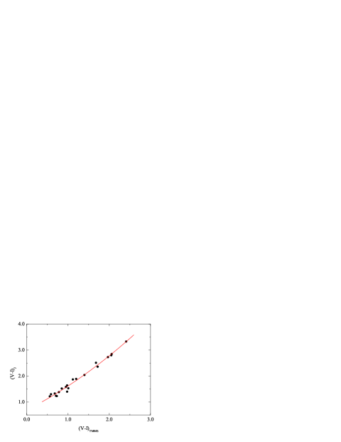
Figure 11: Johnson $(V-I)_{\rm J}$ vs. $(V-I)_{\rm TMMS}$ from the Two Micron Sky Survey catalog of Neugebauer & Leighton (1969). Solid line is the derived relation between $(V-I)_{\rm J}$ and $(V-I)_{\rm TMMS}$ colors (given in numerical form in Eq. 1).

We find slight systematic differences between the $(V-I)_{\rm C}$ colors resulting from $(V-I)_{\rm J}$ and $(V-I)_{\rm TMSS}$. Note that Neugebauer et al. (1965) found no systematic discrepancies between their $I$ magnitudes and those obtained by Kron et al. (1953), at least to within an uncertainty margin of about $\pm 0.2$ mag. The discrepancies that we find are most pronounced at bluer colors (i.e., higher effective temperatures): $\Delta(V-I)\sim 0.20$ at $(V-I)_{\rm TMSS}\sim 0.6$, with Cousins $(V-I)$ colors resulting from $(V-I)_{\rm TMSS}$ being bluer. The differences gradually become smaller for redder colors and diminish at $(V-I)_{\rm TMSS}\ga 2.5$. It should be noted though, that these systematic differences are always within the margin of $\pm 0.2$ mag, which may possibly explain why they were not reported by Neugebauer et al. (1965).

Since these trends may suggest the existence of slight differences in the realization of the TMSS $I$ and standard Kron $I$ passbands (the latter defined by Kron et al. 1957), we used the following procedure to obtain Cousins $(V-I)_{\rm C}$. First, stars from our sample with both $I_{\rm J}$ and $I_{\rm TMSS}$ photometry (20 objects) were used to derive the following relation between $(V-I)_{\rm J}$ and $(V-I)_{\rm TMSS}$:

$$(V-I)_{\rm J}=0.690+0.806(V-I)_{\rm TMSS}+0.1188(V-I)_{\rm TMSS}^{2}$$ (1)

which is valid for $0.5\leq(V-I)_{\rm TMSS}\leq 2.5$. The RMS residual of the fit is 0.086 mag (Fig. 11). This equation was employed to obtain Johnson $(V-I)_{\rm J}$ colors for stars with no Johnson $I$-band photometry available. Then, Johnson $(V-I)_{\rm J}$ colors obtained from $(V-I)_{\rm TMSS}$ and those originally available in the Johnson system were finally transformed to Johnson-Cousins-Glass system using the relations from Fernie (1983).

Near-infrared JK colors were converted to the standard Johnson-Cousins-Glass system using transformations given in Bessell & Brett (1988).

BVIJK colors transformed to the Johnson-Cousins-Glass system, together with references to the original photometry sources, are given in Table 3.

4.3 Interstellar reddening

For most stars in the sample interstellar reddening was derived in the original interferometry/occultation papers, either from the difference between intrinsic (for a given spectral type) and observed broad-band color (D96, D98, VB99), or employing an empirical model of Galactic extinction (DB93). In both cases, the derived interstellar reddenings have been found to be small for the majority of stars; D96, for instance, find a mean color excess of $E(B-V)\sim 0.01$ for all stars in their sample. We thus apply no corrections for interstellar extinction for the observed broad-band colors of stars in our sample.

4.4 Metallicities

A search through the spectroscopic catalogs available in the SIMBAD database has yielded metallicities for 37 (out of 74) stars in our sample. Averaged quantities were used when multiple derivations of $\left[\mathrm{Fe}/\mathrm{H}\right]$ were available (19 objects). For the majority of stars metallicities are close to solar, with a mean $\left[\mathrm{Fe}/\mathrm{H}\right]\simeq-0.16$ and standard deviation of $\simeq$0.20 dex. Indeed, as we use this sample for the comparison with synthetic colors at $\left[\mathrm{Fe}/\mathrm{H}\right]=0.0$, this may result in slight systematic discrepancies, especially in $T_{\rm eff}-(B-V)$ plane. The difference between synthetic $B-V$ colors at $\left[\mathrm{Fe}/\mathrm{H}\right]=0.0$ and $\left[\mathrm{Fe}/\mathrm{H}\right]\sim-0.16$ is $\sim$0.03 mag for $T_{\rm eff}=3800$–5000 K ($T_{\rm eff}$–$\log g$ scale of Houdashelt et al. 2000), with colors at lower metallicity being bluer. The differences for other colors are considerably smaller (typically $\sim$0.01 mag or less). This corresponds to a difference of $\sim$50 K in $T_{\rm eff}$ resulting from $B-V$ at $T_{\rm eff}\geq 3800$ K (less than $\sim$20 K in other colors).

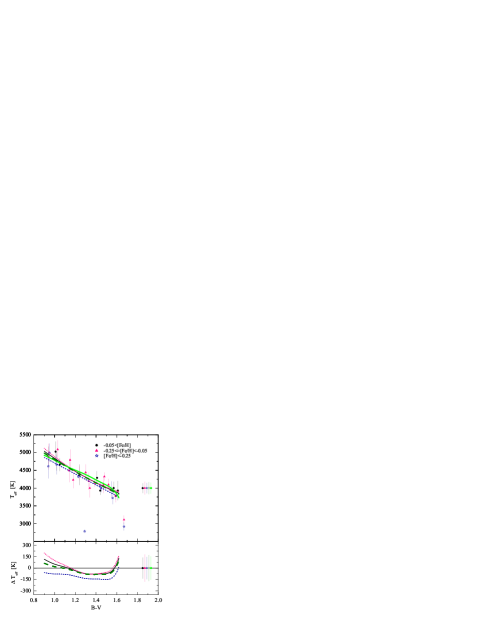
Figure 12: Top: $T_{\rm eff}$–$(B-V)$ diagram for stars with known metallicities. Different symbols stand for the following metallicity bins: circles $\left[\mathrm{Fe}/\mathrm{H}\right]\geq-0.05$ (bin 1), triangles $-0.25\leq\left[\mathrm{Fe}/\mathrm{H}\right]<-0.05$ (bin 2), asterisks $\left[\mathrm{Fe}/\mathrm{H}\right]<-0.25$ (bin 3). Solid, dotted, and short-dashed lines are the best-fits in the metallicity bins 1–3, respectively. Thick long-dashed line is a best-fit to all 37 stars with known metallicities, thick solid line is a best-fit to the entire sample of 74 stars used in our study (see Sect. 4.1 for details). A cluster of symbols with error bars on the right shows the RMS residuals of the corresponding best-fits. Bottom: the difference between the best-fits in various metallicity bins and the best-fit to the sample of 74 stars, $\Delta T_{\rm eff}=T_{\rm eff}^{\rm bin}-T_{\rm eff}^{\rm all}$ (solid, dotted, and short-dashed lines, for the metallicity bins 1–3 respectively). Thick long-dashed line shows the difference between the best-fits to the samples of 37 and 74 stars. RMS residuals of the individual best-fits are shown on the right.

It should be noted though, that we find no clear evidence for the metallicity effects in the $T_{\rm eff}$–color and color–color planes, most likely because the spread in metallicity is small (especially if compared with typical errors in metallicity determinations, e.g., 0.2–0.3 dex). This is illustrated in Fig. 12 which shows the $T_{\rm eff}$–$(B-V)$ relation for 37 stars with known $\left[\mathrm{Fe}/\mathrm{H}\right]$. We divide these 37 stars into three metallicity bins as indicated in the figure and produce the quadratic best-fits for each bin, as well as for the entire sample of 37 stars with available metallicity determinations. The resulting best-fits are shown as solid lines in the upper panel of Fig. 12 (thick dashed line for the sample of 37 stars). We also show a best-fit in the $T_{\rm eff}$–$(B-V)$ plane for the sample containing all 74 stars used in our further analysis (thick solid line; see Sect. 5.1 for details). The RMS residuals of the best-fits are 140 K, 180 K, and 150 K in metallicity bins 1–3 respectively, 150 K for the sample of 37 stars and 170 K for all 74 stars. The mean difference between the best-fit representing the 37 stars and those corresponding to different metallicity bins are 20 K, 40 K and $-$80 K, for bins 1–3 respectively. Thus only the lowest metallicity bin is slightly more deviant, however, in all cases the differences are not statistically significant. Note, however, that the best-fit representing all 37 stars with metallicity determinations is slightly deviant from the best-fit which is based on the entire sample of 74 late-type giants. While the mean difference is small ($-$20 K, with the best-fit for 37 stars predicting lower $T_{\rm eff}$ for a given $B-V$), differences in certain effective temperature ranges may be considerable (e.g., $-$80 K at $T_{\rm eff}\sim 4000$–4400 K), though this is again significantly less than the typical spread of observed $T_{\rm eff}$ in the individual samples.

The differences between the best-fits in individual metallicity bins are considerably smaller in other $T_{\rm eff}$–color and color–color diagrams, with no evident systematical trends.

4.5 Comparison of angular diameters, fluxes and effective temperatures

Figure 13:  Comparison of angular diameters measured by different authors (see text for details). Open circles are the late-type giants used in this work.

Once the angular diameter of a star is known, the effective temperature can be estimated through the following relation (D96):

$$T_{\rm eff}=1.316\times 10^{6}\,\left(\frac{F_{\mathrm{bol}}}{\theta_{\rm R}^{2}}\right)^{1/4}$$ (2)

here $\theta_{\mathrm{R}}$ is the angular diameter (in mas), and F_bol is the bolometric flux (in ${\rm W\,m^{-2}}$). Obviously, potential systematic errors in derived $T_{\rm eff}$ may result both from the differences in derived stellar radii, $\theta_{\rm R}$, and observed bolometric fluxes, $F_{\mathrm{bol}}$.

Bolometric fluxes are usually obtained by integrating observed photometric fluxes over as large wavelength interval as possible. After carefully checking the $F_{\mathrm{bol}}$ given in the original papers (R80, DB93, D96, D98, P98, VB99), we find no significant systematic differences in bolometric fluxes obtained by different groups (exceptions and possible implications are discussed in Sect. 4.5.2). In the forthcoming sections we will thus concentrate on the angular diameters and effective temperatures.

4.5.1 Angular diameters

The measured angular diameter of a star (i.e., a uniform disk diameter, $\theta_{\mathrm{UD}}$) does not exactly represent the true angular diameter and should be corrected for the limb-darkening. This is done by applying a correction (which varies from 1.00 for a uniformly bright disk to $\sim$1.13 for a fully darkened disk), defined as a ratio of the limb-darkened diameter to the uniform disk diameter (at a given wavelength). The correction is derived from stellar atmosphere models (see Scholz & Takeda 1987; Scholz 1997, for a detailed discussion).

The limb-darkened diameter in Eq. (2) is the Rosseland diameter, which corresponds to a surface where the Rosseland mean optical depth is equal to unity. As advocated by Scholz & Takeda (1987), the temperature calculated at this surface provides a good estimate of $T_{\rm eff}$ (see also Baschek et al. 1991 for a more extensive discussion on the definitions of radii and $T_{\rm eff}$ of red giants). Effective temperatures of giants in our sample were derived in the original interferometry papers, employing Rosseland angular diameters which were calculated using the following corrections: $\theta_{\mathrm{R}}\simeq 1.022\theta_{\mathrm{UD}}$ by D96, D98 and VB99; $\theta_{\mathrm{R}}\simeq 1.035\theta_{\mathrm{UD}}$ by P98; similar conversion factors were used for individual stars by DB93 and R80. The Rosseland angular diameters of the sample giants are given in Table 3.

There have been indications discussed in the literature that systematical differences may exist between the uniform disk diameters obtained with different interferometric setups. In their analysis of the Infrared Optical Telescope Array (IOTA) data, D98 have found indications of systematical differences between $\theta_{\mathrm{UD}}$ obtained with the CERGA interferometer (Di Benedetto & Rabia 1987; Di Benedetto & Ferluga 1990) and those obtained with the classical (D98) and FLUOR (P98) beam combiners at IOTA (all operating in the near-infrared $K$-band). To the contrary, a recent comparison of angular diameters obtained with optical interferometers (Mark III and NPOI) has revealed no systematic differences (Nordgren et al. 2001).

The largest fraction of stars used in this work comes from the sample of VB99. However, only three stars in this data set have previous measurements of angular diameters from occultations and interferometry, while none of these three stars is available in the other data sets used in this work. As remarked by VB99, however, angular diameters and effective temperatures of four stars in their sample are in good agreement with those inferred from the infrared flux method. There is also a good agreement with an upper limit estimate for $\theta_{\mathrm{UD}}$ obtained for one of the stars (HR 2630) from lunar occultation. For the two stars with interferometric measurements of $\theta_{\mathrm{UD}}$ the discrepancies are larger, apparently due to large errors in earlier derivations of $\theta_{\mathrm{UD}}$ (see VB99 for a detailed discussion).

A more straightforward comparison can be made for stars from other samples. In Fig. 13 we compare angular diameters from D98 with those derived by DB93, P98, D96, and R80. Stars used in this work are indicated by open circles.

A good agreement can be seen between the samples of D98 and D96; in both cases stars were measured using the same classical beam combiner at IOTA interferometer. There is also a good consistency between angular diameters measured by D98 and P98, who used a FLUOR fiber beam combiner at IOTA; the data scatter however is large. One star, RS Cnc, deviates significantly; however, it is a semiregular variable (of type SRC) with a photographic amplitude of $\sim$1.5 mag (Kholopov et al. 1998, GCVS), thus the discrepancy may also reflect a real variation of stellar diameter. Interestingly, the angular diameter of this star obtained by D96 is also different from that derived by D98 (note that this star is not in the sample used in our study).

The two stars in the sample of R80, RZ Ari and $\lambda$ Aqr, have significantly lower angular diameters than measured by D98. The former is a semiregular variable star of type SRB, with an amplitude of $\Delta V\sim 0.4$ (GCVS), while the latter is an irregular variable of type LB, with $\Delta V\sim 0.1$ (GCVS); at least in the latter case variability alone can not account for the discrepancy.

As it was already indicated by D98, angular diameters measured by DB93 are indeed systematically larger than those obtained by D98 (Fig. 13). There is also a tendency that these differences increase with increasing angular diameter of a star (Fig. 13).

There are two stars in the sample of DB93 which have measurements of angular diameters available from other groups. One star ($\mu$ Gem) was observed by R80; the DB93 value (originaly measured by Di Benedetto & Rabia 1987), $13.50\pm 0.15$ mas, is indeed larger than that obtained by R80, $12.10\pm 0.39$ mas. The other star is $\alpha$ Tau, which was measured by P98. In this case the obtained angular diameters agree well, with $19.60\pm 0.29$ mas obtained by DB93 and $19.75\pm 0.11$ mas by P98.

Obviously, the largest systematic discrepancies arise between the data sets of DB93 and D98; angular diameters of five stars obtained by DB93 tend to be larger than those derived by D98. The measured radii of the two stars common to D98 and R80 are rather discrepant too, as are the measurements of RS Cnc by D98 and P98. Note that the scatter of the individual measurements in Fig. 13 is generally large. This is perhaps even more surprising, as the majority of these stars are non-variable and in some cases their angular diameters are measured using the same instrument.

Figure 14:  Comparison of effective temperatures measured by different authors (see text for details). Open circles are the late-type giants used in this work.

While pinning down the precise source of these discrepancies is beyond the scope of this study, several comments may be appropriate. First, it should be noted that angular diameters quoted in DB93 are taken from the earlier study of Di Benedetto & Rabia (1987), with the original interferometric measurements obtained more than two decades ago. The angular diameters derived in Di Benedetto & Rabia (1987) are thus amongst the pioneering interferometric measurements of the angular diameters of late-type giants, with typically large uncertainties in the data reduction procedure (calibration, conversion from the uniform to limb-darkened angular diameters, and so forth). Second, angular diameters in D98 were mostly derived from a single observation of the visibility made at one spatial frequency point, which clearly may introduce additional systematic uncertainties. For instance, according to Wittkowski et al. (2004) visibility function of the late-type giant $\psi$ Phe measured with the VLTI/VINCI is significantly different from both the uniform disk and fully-darkened disk models, but it seems that this discrepancy is clearly discerned only in the second lobe of the visibility function.

Indeed, stars that are common to different data sets used in our study are too few to decide firmly whether the discrepancies mentioned above point towards the general systematic differences, or they simply show the scatter due to small number statistics. Nevertheless, all these differences clearly indicate that the real errors in the measured stellar radii may be considerably larger than indicated by the error bars provided in the individual studies. Inevitably, this has a direct effect on the effective temperatures derived using the observed stellar radii, thus putting a lower limit on the data scatter in observed $T_{\rm eff}$–color relations.

4.5.2 Effective temperatures

Effective temperatures calculated in the original interferometry papers (R80, DB93, D96, D98, P98, VB99) are given in Table 3. A comparison of $T_{\rm eff}$ derived by different groups is shown in Fig. 14, with stars used in this work indicated by open circles.

As in the case of angular diameters, the agreement in $T_{\rm eff}$ derived by D98 and D96 is very good. It should be mentioned though, that identical values of $F_{\mathrm{bol}}$ were used in both studies, thus the consistency in derived $T_{\rm eff}$ simply reflects the agreement in derived angular diameters.

Effective temperatures derived by P98, however, tend to be systematically lower than those obtained by D98. This is determined either by a larger angular diameter ($\delta$ Oph), smaller $F_{\mathrm{bol}}$ (RX Boo, BK Vir), or both (EU Del, $\tau^{4}$ Ser), as derived by P98. While both angular diameter and $F_{\mathrm{bol}}$ are significantly deviating in case of RS Cnc, both quantities are smaller than those derived by D98 by a similar factor, thus leaving the resulting $T_{\rm eff}$ unaltered.

Effective temperatures derived by DB93 also tend to be systematically lower than those of D98. This is a consequence of systematically larger angular diameters of DB93. The $T_{\rm eff}$ of $\lambda$ Aqr derived by R80 is significantly higher ($\Delta T_{\rm eff}\sim 270$ K) than that obtained by D98, which is a consequence of considerably smaller angular diameter derived by R80.

The discrepancies in $T_{\rm eff}$ derived by various groups are thus non-negligible, and result from the differences both in angular diameters (predominantly) and bolometric fluxes. Effective temperatures of stars in the samples of P98 and DB93 seem to be systematically lower than those obtained by D98. A comparison of general trends of stars from different samples in the $T_{\rm eff}$–color diagrams gives an indication that the $T_{\rm eff}$ derived by D98 are somewhat higher ($\sim$50 K) than the average trend of the sample including all 74 stars, while the effective temperatures of P98 and DB93 tend to be lower by a comparable amount.

To investigate a possible effect of these systematic differences on the $T_{\rm eff}$–color and color–color relations derived in Sect. 5, we produced $T_{\rm eff}$–color scales in different color planes without including stars from the sample of D98 (while using all stars from the other samples). This procedure was repeated by excluding each sample in turn from the whole sample of 74 stars. In all cases, the resulting $T_{\rm eff}$–color relations were essentially unaltered. Typically, the differences between the $T_{\rm eff}$–color relations based on all 74 stars and those with stars from a certain sample excluded were within $\sim$70 K for $T_{\rm eff}=3700$–4800 K, suggesting that the influence of these systematical differences on the derived $T_{\rm eff}$–color relations is small.

5 Synthetic photometric colors versus observations: results and discussion

Since precise effective temperatures and broad-band photometric colors of late-type giants in the solar neighborhood are readily available, they can be supplemented with the $T_{\rm eff}$–$\log g$ relation to construct an empirical $T_{\rm eff}$–$\log g$–color scale based on the observed quantities of late-type giants (Table 3). This scale could be used further to make a direct comparison of the new synthetic colors with the observations of late-type giants in our sample, as well as with available $T_{\rm eff}$–color and color–color relations. It may also provide a basis for checking the consistency between synthetic colors calculated with different model atmosphere codes.

5.1 New $T_{\rm eff}$–$\log g$–color scales

Although no previous knowledge about the evolutionary status of stars in Table 3 is available, it is most likely that these stars are either on the red giant branch (RGB), or asymptotic giant branch (AGB). Obviously, their gravities and effective temperatures have to be related through the appropriate $T_{\rm eff}$–$\log g$ relations, which should ideally be different for stars on the RGB and AGB.

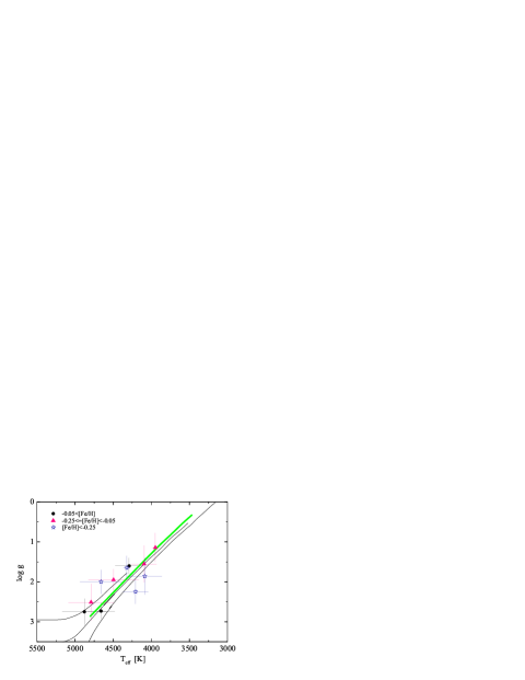
Figure 15: Stars from Table 3 with spectroscopic gravities available from the literature plotted in the $T_{\rm eff}$–$\log g$ plane. Symbols mark the following metallicity bins: circles $\left[\mathrm{Fe}/\mathrm{H}\right]\geq-0.05$, triangles $-0.25\leq\left[\mathrm{Fe}/\mathrm{H}\right]<-0.05$, asterisks $\left[\mathrm{Fe}/\mathrm{H}\right]<-0.25$. Thick solid line corresponds to the $T_{\rm eff}$–$\log g$ scale of Houdashelt et al. (2000a, H00) extrapolated linearly to $T_{\rm eff}=4800$ K. Thin lines are isochrones of Marigo & Girardi (2001) for 0.5, 2 and 10 Gyr.

Unfortunately, the present knowledge about the variations of $\log g$ along the RGB and AGB is rather limited, and relies essentially on theoretical modeling. Since empirical $\log g$ of RGB and AGB stars are typically a product of spectroscopic analysis, their determination becomes extremely complicated at effective temperatures lower than $\sim$4000 K (due to problems related with the definition of continuum, effects of line overlapping, etc.), uncertainties that grow sharply with decreasing $T_{\rm eff}$. Effects of metallicity and age may introduce additional scatter/shifts in the resulting $T_{\rm eff}$–$\log g$ scale. Though these uncertainties indeed place internal limitations on the precision of existing $T_{\rm eff}$–$\log g$ calibrations, more importantly, any empirical $T_{\rm eff}$–$\log g$ scale is likely to suffer from these uncertainties in a systematical way too, depending on the properties of the stellar sample from which it was derived.

Thus, ideally, we would like to construct a $T_{\rm eff}$–$\log g$ scale which is based entirely on the observed quantities of stars from our sample. However, only 11 stars from Table 3 have spectroscopic gravities available from the literature. When plotted on the $T_{\rm eff}$–$\log g$ plane (Fig. 15), the scatter in the data is too large to derive a reliable temperature–gravity relation.

For the purposes of this study we thus use one of the existing empirical $T_{\rm eff}$–$\log g$ relations, namely the scale of Houdashelt et al. (2000a, H00), which is based on the effective temperatures derived from interferometry and gravities assigned from theoretical isochrones (see H00 for details). According to Houdashelt et al. (2000a, b), synthetic broad-band colors based on their $T_{\rm eff}$–$\log g$ relation agree well with observations of nearby K and early-M giants in the $T_{\rm eff}$–color planes. Their relation is also in reasonable agreement with observations of 11 giants from our sample (Fig. 15), although the scatter in the observed data is indeed large.

Table 4: New empirical $T_{\rm eff}$–$\log g$–color relation for the late-type giants. The $T_{\rm eff}$–color relations are best-fits to the observed effective temperatures and colors of 74 late-type giants, while gravities are assigned to a given $T_{\rm eff}$ according to the $T_{\rm eff}$–$\log g$ relation of Houdashelt et al. (2000a, H00). The last line gives the RMS residual of the fit, expressed as a temperature difference. Photometric colors are in the Johnson-Cousins-Glass system (see Sect. 5.1 for more details).

$T_{\rm eff}$	$\log g$		$B\!-\!V$	$V\!-\!I$	$V\!-\!K$	$J\!-\!K$
4800	2.90		1.021	1.016	2.280	0.639
4700	2.69		1.075	1.054	2.392	0.675
4600	2.49		1.133	1.096	2.514	0.712
4500	2.28		1.195	1.144	2.649	0.750
4400	2.08		1.263	1.198	2.798	0.789
4300	1.89		1.338	1.261	2.963	0.828
4200	1.69		1.408	1.334	3.146	0.869
4100	1.50		1.469	1.421	3.350	0.910
4000	1.30		1.528	1.526	3.580	0.952
3900	1.11		1.573	1.648	3.839	0.996
3800	0.93		1.605	1.786	4.133	1.040
3700	0.74		1.622	1.962	4.469	1.086
3600	0.57		1.628	2.192	4.855	1.133
3500	0.39		1.630	2.501	5.304	1.181
RMS residual [K]			170	160	140	150

Table 5: Semi-empirical $T_{\rm eff}$–$\log g$–color relations for late-type giants based on synthetic colors calculated with PHOENIX and MARCS model atmospheres. Photometric colors are given in the Johnson-Cousins-Glass system (see Sect. 5.1 for details).

			PHOENIX				MARCS
$T_{\rm eff}$	${\rm log}\,g$		$B\!-\!V$	$V\!-\!I$	$V\!-\!K$	$J\!-\!K$	$B\!-\!V$	$V\!-\!I$	$V\!-\!K$	$J\!-\!K$
4800	2.90		1.054	1.060	2.333	0.607	1.056	1.013	2.323	0.626
4700	2.69		1.103	1.105	2.445	0.639	1.109	1.054	2.431	0.658
4600	2.49		1.150	1.152	2.562	0.673	1.164	1.100	2.547	0.693
4500	2.28		1.204	1.205	2.690	0.709	1.222	1.150	2.672	0.729
4400	2.08		1.259	1.263	2.827	0.748	1.284	1.206	2.805	0.767
4300	1.89		1.315	1.329	2.975	0.789	1.345	1.267	2.950	0.808
4200	1.69		1.370	1.402	3.136	0.831	1.406	1.334	3.106	0.853
4100	1.50		1.421	1.485	3.312	0.875	1.466	1.411	3.276	0.900
4000	1.30		1.473	1.587	3.512	0.921	1.529	1.506	3.468	0.947
3900	1.11		1.516	1.710	3.739	0.969	1.582	1.621	3.686	0.996
3800	0.93		1.551	1.860	4.002	1.017	1.619	1.765	3.940	1.046
3700	0.74		1.573	2.056	4.321	1.064	1.636	1.950	4.245	1.096
3600	0.57		1.563	2.324	4.736	1.113	1.617	2.201	4.631	1.147
3500	0.39		1.505	2.707	5.319	1.160	1.556	2.543	5.139	1.197

We provide several new $T_{\rm eff}$–$\log g$–color scales. Table 4 gives an empirical $T_{\rm eff}$–$\log g$–color relation derived using empirical $T_{\rm eff}$–color relations (thick lines in Fig. 16) obtained as best-fits to the observed data (stars from Table 3, except those from the sample of P98) and supplemented with the $T_{\rm eff}$–$\log g$ scale of H00. The H00 scale used for this purpose was linearly extrapolated to $T_{\rm eff}=4800$ K. The typical RMS error of the fitting procedure is $\sim$160 K (Table 4). Tables 5–6 list three additional semi-empirical scales, based on synthetic colors of PHOENIX, MARCS and ATLAS corresponding to the $T_{\rm eff}$–$\log g$ relation of H00. All scales are valid for the effective temperature range of $T_{\rm eff}=3500$–4800 K. It should be noted that the H00 scale is representative of RGB stars, thus appropriate care should be taken when using these new $T_{\rm eff}$–$\log g$–color relations both at the low and high effective temperature ends, where RGB stars may be mixed with objects on the horizontal branch and AGB, respectively.

The scatter in observational data may provide an estimate of the intrinsic limits in the precision of empirical $T_{\rm eff}$–color relations, as indicated, for instance, by RMS residuals of the best fits to the observed sequences of late-type giants in various $T_{\rm eff}$–color planes. These errors are typically $\sim$160 K (Table 4) and they are determined by the current uncertainties in interferometrically derived effective temperatures, various systematical effects, astrophysical scatter, etc.

5.2 Comparison of $T_{\rm eff}$–color relations

Table 6: Semi-empirical $T_{\rm eff}$–$\log g$–color relation for late-type giants based on synthetic colors calculated with ATLAS model atmospheres. Photometric colors are given in the Johnson-Cousins-Glass system (see Sect. 5.1 for details).

			ATLAS
$T_{\rm eff}$	${\rm log}\,g$		$B\!-\!V$	$V\!-\!I$	$V\!-\!K$	$J\!-\!K$
4750	2.79		1.067	1.051	2.391	0.650
4500	2.28		1.191	1.165	2.685	0.740
4250	1.79		1.330	1.308	3.035	0.842
4000	1.30		1.497	1.512	3.472	0.955
3750	0.84		1.648	1.831	4.060	1.071
3500	0.39		1.683	2.396	4.974	1.173

Synthetic PHOENIX, MARCS and ATLAS colors given in Tables 5–6 provide three new semi-empirical $T_{\rm eff}$–color scales which may be readily compared with the observations of giants from Table 3 in the $T_{\rm eff}$–color and color–color domains. This also gives a possibility for a direct comparison between the PHOENIX, MARCS and ATLAS colors, since they are all given for the same $T_{\rm eff}$–$\log g$ relation of H00. A comparison of the new relations with observations and published $T_{\rm eff}$–color scales is given in Fig. 16.

In order to provide a reference frame for discussion of the new scales, we also include the following recently published $T_{\rm eff}$–color relations into our analysis:

• BaSeL 2.2 (Lejeune et al. 1998, BaSeL 2.2): photometric colors are derived from theoretical spectra calibrated to match empirical $T_{\rm eff}$–color relations at $\left[\mathrm{Fe}/\mathrm{H}\right]=0.0$. BaSeL 2.2 colors used in this work were calculated for the $T_{\rm eff}$–$\log g$ relation of H00, using the interactive web-based BaSeL server ;

• Alonso et al. (1999, A99): empirical scale, obtained using photometric observations of a large sample of Galactic field and globular cluster stars at different metallicities. Effective temperatures of individual stars were derived using the infrared flux method (IRFM), the best-fits yielding $T_{\rm eff}$–color and color–color relations;

• Sekiguchi & Fukugita (2000, SF00): empirical $T_{\rm eff}$–$(B-V)$ scale, obtained using observed colors and effective temperatures of 537 Infrared Space Observatory (ISO) standard stars from Di Benedetto (1998). Effective temperatures of individual stars were derived from the $T_{\rm eff}$–$(V-K)$ relation, calibrated on a sample of nearby stars with angular diameters available from interferometry. For the purposes of this study their $B-V$ colors were selected according to the $T_{\rm eff}$–$\log g$ relation of H00;

• Vandenberg & Clem (2003, VC03): empirical scales based on synthetic BVRI colors of Bell & Gustafsson (1978, 1989), adjusted to satisfy observational constrains from the CMDs of several Galactic globular and open clusters, field stars in the solar neighborhood, empirical $T_{\rm eff}$–color relations, etc. We used VC03 colors selected according to the $T_{\rm eff}$–$\log g$ scale of H00;

• Houdashelt et al. (2000a, H00): theoretical colors, calculated with MARCS and SSG codes; TiO opacities were adjusted to reproduce the observed spectra of M giants from Fluks et al. (1994); no ${\rm H_{2}O}$ opacities were included in the calculations. Their photometric colors are given for the H00 $T_{\rm eff}$–$\log g$ relation (provided in the same paper), which was linearly extrapolated by us to $T_{\rm eff}=4800$ K;

• Sviderskienė (1988, S88), Pickles (1998, Pi98): scales based on photometric colors calculated from the observed spectra of late-type giants. Note that observed spectra from Pi98 and S88 are compared with those calculated using PHOENIX and MARCS model atmospheres in Sect. 5.4, thus the two scales are provided to illustrate the behaviour of photometric colors in the $T_{\rm eff}$–color planes. Photometric colors of the S88 and Pi98 scales were calculated by us in the standard Johnson-Cousins-Glass photometric system using the procedure described in Sect. 2.3. Effective temperatures for both scales were assigned using the effective temperature – spectral class relation of Pi98;

  

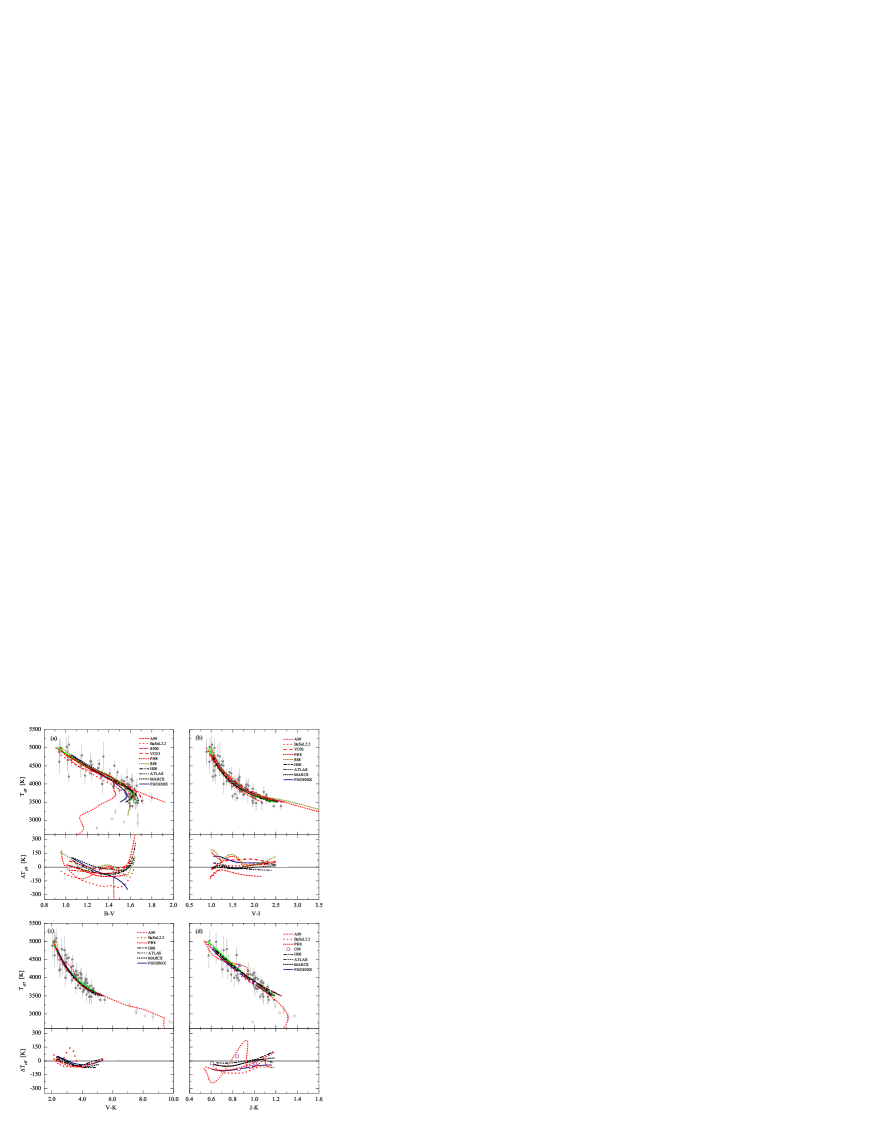
  Figure 16: Empirical and theoretical $T_{\rm eff}$–color relations for late-type giants in different $T_{\rm eff}$–color planes (a–d, top panels). Filled circles are late-type giants from Table 3, stars from the sample of Perrin et al. (1998) are highlighted as open circles. Thick solid line is a best-fit to the data, which represents a new empirical $T_{\rm eff}$–$\log g$–color scale (Table 4) in a particular $T_{\rm eff}$–color plane. Several existing $T_{\rm eff}$–color relations are shown as well, together with semi-empirical scales constructed using synthetic colors of PHOENIX, MARCS and ATLAS (Table 5). Open rectangles in panel (d) are late-type giants from Cohen et al. (1999) (see text for details). Bottom panels in each figure show the difference between various $T_{\rm eff}$–color relations and the empirical scale (thick solid line, Table 4) in a given $T_{\rm eff}$–color plane ($\Delta T_{\rm eff}=T_{\rm eff}^{\rm other}-T_{\rm eff}^{\rm bestfit}$).

• Cohen et al. (1999, C99): photometric colors of the five late-type giants used by Cohen et al. (1999) in the role of templates to produce a library of near-infrared spectra of late-type giants (a comparison of several C99 spectra with those produced using stellar model atmospheres is given in Sect. 5.4). The five late-type giants are: $\beta$ Gem (K0 III; spectrum taken from Cohen et al. 1995); $\alpha$ Boo (K1.5 III; Cohen et al. 1996); $\alpha$ Hya (K3 III; Cohen et al. 1995); $\alpha$ Tau (K5 III; Cohen et al. 1999); and $\beta$ And (M0 III; Cohen et al. 1995). Effective temperatures of individual stars were taken either from Table 3, or from Cohen et al. (1995, 1996, 1999). Observed $J-K$ colors were collected from the literature (typically – SIMBAD database) and converted to the standard Johnson-Cousins-Glass system using transformations given in Bessell & Brett (1988).

It should be noted, that A99 give an extensive comparison of their scale with existing $T_{\rm eff}$–color relations; similar comparisons are also done by SF00 and VC03. Altogether this may provide a further reference for a comparison of the new scales derived in this work with other relations published in the literature.

Generally, the consistency between different $T_{\rm eff}$–color relations (including those based on synthetic colors of PHOENIX, MARCS and ATLAS) and observed sequences of late-type giants (represented by the new empirical scales in Tables 5–6) is good over a large range of effective temperatures (or colors). The agreement is especially good in the $T_{\rm eff}$–$(V-K)$ plane (Fig. 16c), where all scales agree to within $\Delta T_{\rm eff}\sim 80$ K. The only exception is the scale of Pi98 which predicts considerably higher effective temperatures in the range of $T_{\rm eff}\sim 4000-4400$ K (a similar ’bump’ in the $T_{\rm eff}$–color relations based on Pi98 colors can also be seen in the $T_{\rm eff}$–$(V-I)$ and $T_{\rm eff}$–$(J-K)$ planes). It is quite possible, however, that the effective temperatures of Pi98 giants are slightly overestimated in this $T_{\rm eff}$ range (see Sect. 5.4 for details).

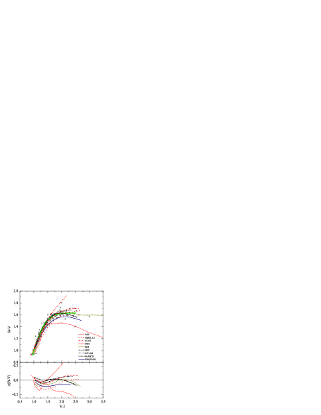
Figure 17: (a) Top: Empirical and theoretical color–color relations in the $(B-V)$–$(V-I)$ plane. Filled circles are late-type giants from Table 3. The thick green line is a new empirical $(B-V)$–$(V-I)$ scale (Table 4; note that it is derived from the individual best-fits in the $T_{\rm eff}$–$(B-V)$ and $T_{\rm eff}$–$(V-I)$ planes, i.e., it is not a best-fit in the $(B-V)$–$(V-I)$ plane). Several existing $T_{\rm eff}$–$(B-V)$ relations are also shown. Bottom: the difference between various $(B-V)$–$(V-I)$ relations and the new empirical scale, $\Delta T_{\rm eff}=T_{\rm eff}^{\rm other}-T_{\rm eff}^{\rm bestfit}$.

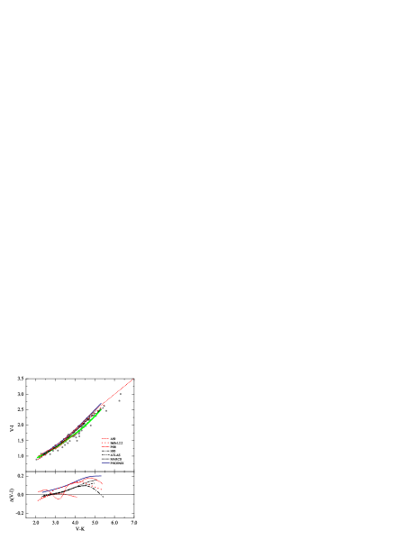
Figure 17: (b) Same as Fig. 17a but in the $(V-I)$–$(V-K)$ plane.

Discrepancies are also small in the $T_{\rm eff}$–$(J-K)$ plane (Fig. 16d), where deviations do not exceed $\pm 100$ K within $T_{\rm eff}=3500$–4500 K (with the exception of the scales based on Pi98 and BaSeL 2.2. colors). There is a hint however, that our new empirical scale tends to predict slightly higher effective temperatures for $(J-K)\sim 0.6$–1.0 than other existing scales. A slightly larger spread of different $T_{\rm eff}$–color scales is seen in the $T_{\rm eff}$–$(V-I)$ plane, though differences between the new empirical $T_{\rm eff}$–$(V-I)$ scale and other existing relations generally are within $\pm 120$ K (the $T_{\rm eff}$–color relations based on Pi98, S88, and BaSeL 2.2 colors are somewhat more deviant).

The situation is more complex in the $T_{\rm eff}$–$(B-V)$ plane (Fig. 16a), where different scales start to diverge below $\sim$4000 K. These deviations are most obviously due to inconsistencies in reproducing the ‘turn-off’ towards the bluer colors seen in the observed data at $(B-V)\sim 1.65$ ($T_{\rm eff}\sim 3600$ K) caused by the increasing absorption in TiO bands. The majority of $T_{\rm eff}$–$(B-V)$ relations agree well with the new empirical scale down to $\sim$3800 K (or $(B-V)\sim 1.6$), the typical deviations being well within $\pm 100$ K. The deviations are even smaller in case of VC03 scale ($\pm 50$ K down to $\sim$3900 K). It should be noted in this respect that theoretical isochrones of Bergbusch & Vandenberg (2001) transformed to observational planes using VC03 $T_{\rm eff}$–color relations are in excellent agreement with the observed CMDs of Galactic globular and open clusters, and field stars in the solar neighborhood (VC03).

However, the agreement is considerably poorer in the case of $T_{\rm eff}$–$(B-V)$ scales based on PHOENIX and BaSeL 2.2 colors. The former starts to deviate at $\sim$4100 K, while the latter is discrepant by more than $\sim$100–200 K within the entire effective temperature range of interest. The scale based on Pi98 colors shows significant deviations as well. These grow especially large below $T_{\rm eff}\sim 4000$ K, where the Pi98 scale essentially fails to reproduce the observations and is at odds with the other $T_{\rm eff}$–$(B-V)$ relations too. This fact is rather disturbing, especially as the Pi98 scale has difficulties in reproducing the observed colors of late-type giants in other $T_{\rm eff}$–color planes too. Since the spectral library of Pickles (1998) is widely used in a variety of astrophysical applications (e.g., the modelling of integrated colors of stellar populations), these inconsistencies should be properly taken into account. Finally, we should stress that none of the existing $T_{\rm eff}$–$(B-V)$ scales reproduces trends in the observed data correctly below $\sim$3800 K. The only exception in this sense is perhaps the scale based on S88 colors, though it predicts the turn-off towards the bluer $B-V$ at slightly higher effective temperatures than hinted from the observations of late-type giants in our sample.

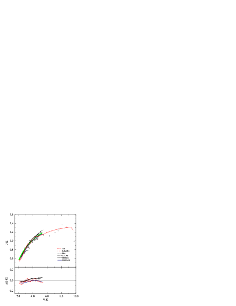
Figure 17: (c) Same as Fig. 17a but in the $(J-K)$–$(V-K)$ plane. Stars from the sample of Perrin et al. (1998) are highlighted as open circles.

It should be remembered that $T_{\rm eff}$–$\log g$–color scales employing synthetic broad-band colors (PHOENIX, MARCS, ATLAS) are indeed sensitive to the $T_{\rm eff}$–$\log g$ scale used, especially at lower effective temperatures. A shift in gravity of $\Delta\log g=\pm 0.2$ at $T_{\rm eff}=3500$ K would produce a shift $\Delta(B-V)\sim\pm 0.04$ and $\Delta(V-I)\sim\Delta(V-K)\sim\pm 0.03$ (redder colors for lower gravities), with smaller differences for other colors. This would correspond to differences of $\Delta T_{\rm eff}\sim 50$ K for $B-V$ and $\Delta T_{\rm eff}\la 10$ K for $V-I$ and $V-K$. Note that these differences will be generally smaller at higher effective temperatures, because of the weaker sensitivity of the emerging spectral flux on gravity. While these effects may be important in the $T_{\rm eff}$–$(B-V)$ plane, they are indeed too small to influence the differences between different $T_{\rm eff}$–color relations involving other photometric colors.

It is interesting to note, that synthetic colors of PHOENIX, MARCS, ATLAS and H00 agree to within $\Delta T_{\rm eff}\sim 100$ K over a large range of effective temperatures, despite the fact that PHOENIX models assume spherical geometry while colors of MARCS, ATLAS and H00 are calculated using plane-parallel model atmospheres. All of them also show a reasonably good agreement with the observed colors of late-type giants (to about $\sim 150$ K).

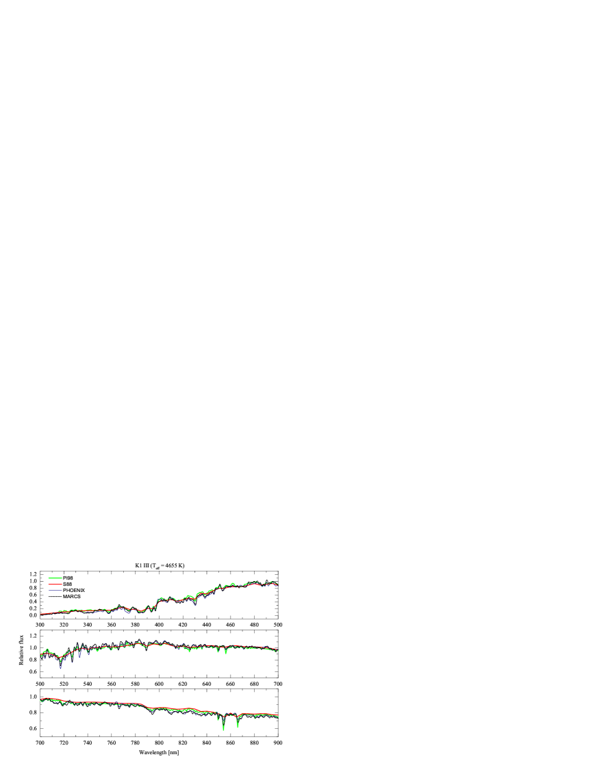
Figure 18:  Comparison of observed spectra from the spectral libraries of S88 and Pi98 with those calculated using PHOENIX and MARCS model atmospheres, for K1 III giant ($T_{\rm eff}=4655$ K, $\left[\mathrm{Fe}/\mathrm{H}\right]=0.0$; the metallicity of Pi98 spectrum is $\left[\mathrm{Fe}/\mathrm{H}\right]=0.09$). Surface gravity in theoretical models was assigned according to the $T_{\rm eff}$–$\log g$ scale of H00 ($\log g=2.60$). Note the different y-scale in different panels.

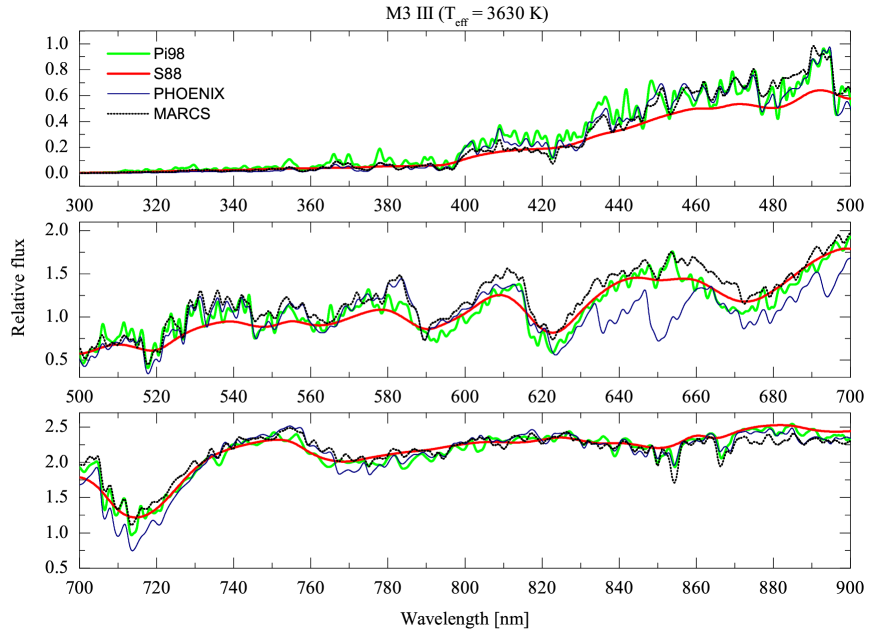
Figure 19:  Same as in Fig. 18 but for a M3 III giant ($T_{\rm eff}=3630$ K, $\log g=0.62$, $\left[\mathrm{Fe}/\mathrm{H}\right]=0.0$).

5.3 Comparison of color–color relations

The comparison of different color–color relations is given in Figs. 17a–c. Empirical color–color relations shown there are constructed from $T_{\rm eff}$–color relations given in Table 4, thus they do not represent the best-fits to the observed data in color–color diagrams.

The most complex behavior is seen in the $(B-V)$–$(V-I)$ plane. While the agreement between different color–color scales is generally rather good at higher effective temperatures (with the exception of scale based on BaSeL 2.2 colors), discrepancies become larger at lower $T_{\rm eff}$, which is to a large extent determined by the discrepancies in the $T_{\rm eff}$–$(B-V)$ plane. For instance, the scale of A99 deviates rapidly beyond $(B-V,V-I)\leavevmode\nobreak\ \sim\leavevmode\nobreak\ (1.5,1.5)$, and the Pi98 scale is strongly deviant beyond $(B-V,V-I)\leavevmode\nobreak\ \sim\leavevmode\nobreak\ (1.4,1.4)$, as both of them fail to reproduce the ‘turn-off’ in the $T_{\rm eff}$–$(B-V)$ plane. All three scales that are based on synthetic colors (Tables 5–6) display slightly differing trends, though they all agree with the observed colors of late-type giants to within $\pm 0.1$ mag (or less) in $B-V$. Note, however, that the scale based on PHOENIX colors is slightly too blue in $B-V$ throughout the entire effective temperature range, which is again a consequence of the discrepancies in the $T_{\rm eff}$–$(B-V)$ plane. Interestingly, the scale based on colors calculated from the observed spectra of S88 shows a remarkably good agreement with the observations in the entire color–color range.

There seem to be some inconsistencies between observed and synthetic $V-I$ colors within the entire effective temperature range in the $T_{\rm eff}$–$(V-I)$ and $(V-I)$–$(V-K)$ planes, as scales based on synthetic colors develop a systematical shift towards the redder $(V-I)$ for a given value of $(V-K)$. This effect is most pronounced for the PHOENIX colors, largely due to a somewhat discrepant trend in the $T_{\rm eff}$–$(V-I)$ plane. BaSeL 2.2 and Pi98 colors follow similar pattern. It is rather unlikely though that these differences are due to the systematical differences between the $I$-band magnitudes in the Two-Micron Sky Survey and standard Kron systems (Sect. 4.2), since the largest systematical discrepancies are seen for the bluer colors and they gradually diminish for the redder, while the differences in Fig. 17b are largest for the reddest stars. The good agreement of the A99 scale with observed trends is somewhat misleading. Since this scale is systematically shifted towards the lower $T_{\rm eff}$ by a comparable amount both in the $T_{\rm eff}$–$(V-I)$ and $T_{\rm eff}$–$(V-K)$ planes, these differences compensate for each other and produce a good agreement of the A99 scale with observations in the $(V-I)$–$(V-K)$ plane.

Excellent agreement is seen again in color–color diagrams involving near-infrared colors; differences between various color–color relations are typically within $\Delta(J-K)=0.1$ in the $(J-K)$–$(V-K)$ plane. This fact is rather remarkable, especially if taken into account that spectra of late-type giants are influenced by a number of strong molecular bands (TiO, CO, ${\rm H_{2}O}$, VO, CO, etc.) in this wide wavelength range.

5.4 Comparison of observed and synthetic spectra

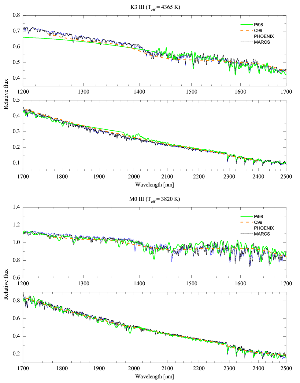
Figure 20:  Comparison of the near-infrared observed spectra from the spectral libraries of Pi98 and C99 with those calculated using PHOENIX and MARCS model atmospheres, for K3 III ($T_{\rm eff}=4365$ K, top) and M0 III ($T_{\rm eff}=3820$ K, bottom) giants. To make the comparison easier, spectra are renormalized to yield the same total flux in the wavelength interval covered by the C99 spectrum. All spectra are of solar metallicity except K3 III of Pi98 ($\left[\mathrm{Fe}/\mathrm{H}\right]=-0.02$). Surface gravity in theoretical models was assigned according to the $T_{\rm eff}$–$\log g$ scale of H00 ($\log g=2.01$ and $\log g=0.97$ for K3 III and M0 III, respectively).

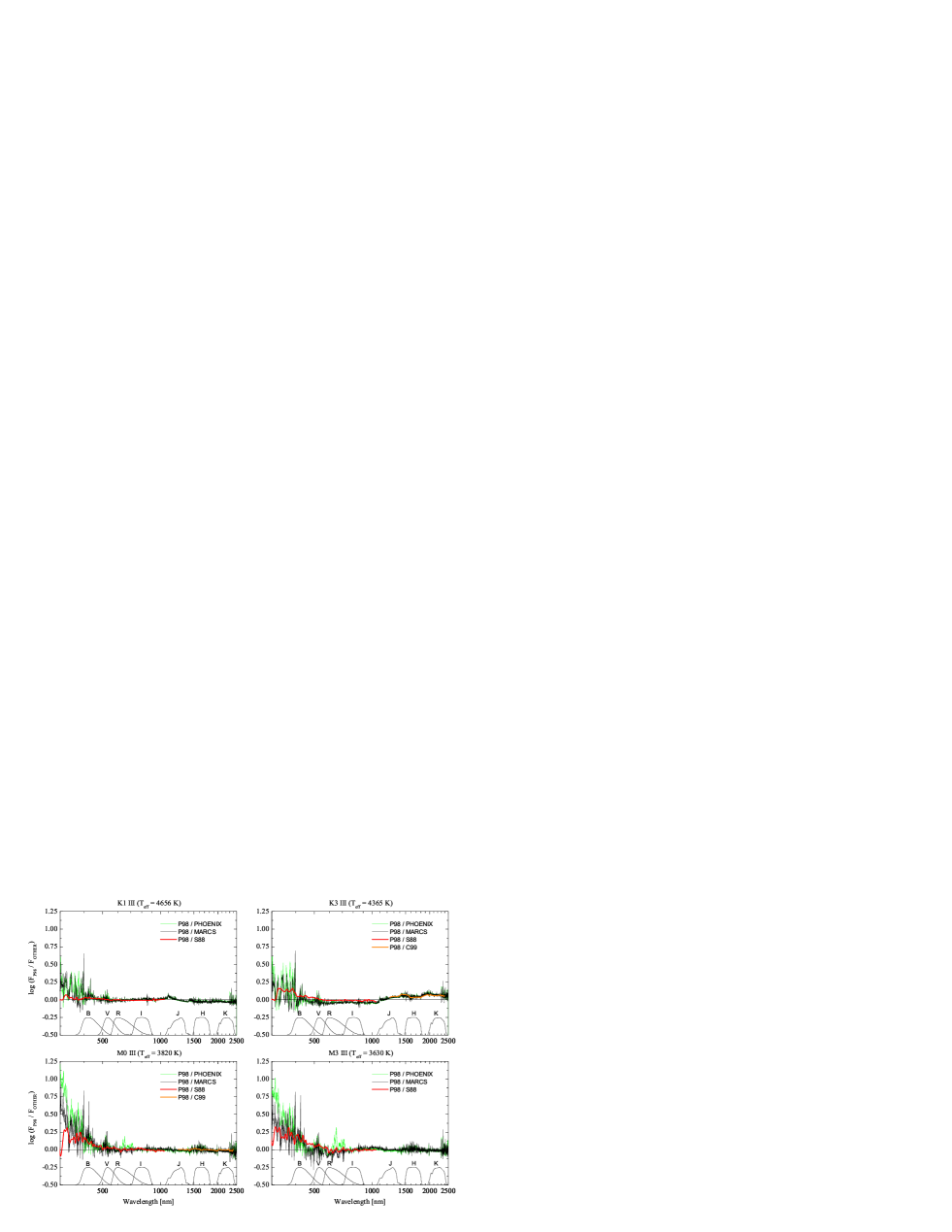
Figure 21:  Spectral flux ratios of Pi98 spectra over the other observed (S88, C99) and synthetic (PHOENIX, MARCS) spectra.

Perhaps the most direct way to clarify what causes the differences between the observed photometric colors of late-type giants and synthetic colors calculated with different stellar model atmospheres is by making a comparison of observed and synthetic spectra.

Examples of the observed optical spectra from the spectral libraries of S88 and Pi98, together with those calculated with the PHOENIX and MARCS model atmospheres are shown in Figs. 18-19, for late-type giants of spectral classes K1 III ($T_{\rm eff}=4655$ K, according to the spectral class–effective temperature relation used in Pi98) and M3 III ($T_{\rm eff}=3630$ K). The observed spectra of Pi98 correspond to the metallicities of $\left[\mathrm{Fe}/\mathrm{H}\right]=0.09$ and $\left[\mathrm{Fe}/\mathrm{H}\right]=0.0$ for the spectral types K1 III and M3 III, S88 spectra are of solar metallicity. Synthetic spectra are all calculated at solar metallicity, for the effective temperatures corresponding to the two spectral classes and with gravities assigned according to the $T_{\rm eff}$–$\log g$ relation of H00 ($\log g=2.60$ and $\log g=0.62$, for K1 III and M3 III, respectively). Synthetic spectra are degraded to a resolution of 1 nm (which corresponds to a typical resolution in the Pi98 library), and then are normalized in such a way that they yield the same total flux as the corresponding Pi98 spectrum in the wavelength interval covered by the latter. S88 spectra are normalized to yield the same flux as Pi98 spectra in the wavelength interval covered by S88 spectra. Note that resolution of S88 spectra ($\sim 5$ nm) is certainly too low for making a detailed comparison on the level of individual spectral lines/bands. Nevertheless, they are still useful for the comparison of general trends, especially given the fact that $T_{\rm eff}$–color relations based on photometric colors of late-type giants in S88 are in excellent agreement with the observations and other $T_{\rm eff}$–color scales in the $T_{\rm eff}$–$(B-V)$ plane. Similarly, Fig. 20 illustrates the situation in the infrared part of the spectrum, for the spectral types of K3 III and M0 III. Here, we also show infrared spectra of two late type giants from the spectral library of C99: $\alpha$ Hya (K3 III; the original spectrum taken from Cohen et al. 1995) and $\beta$ And (M0 III; Cohen et al. 1995). Note that all spectra in Fig. 20 are normalized in such a way that they yield the same total flux over the wavelength interval covered by the C99 spectrum (1240–2400 nm in case of K3 III and 1240–2500 nm in case of M0 III). Finally, Fig. 21 shows the flux ratios of Pi98 spectra over the other observed (S88, C99) and synthetic (PHOENIX, MARCS) spectra (the y-scale in Fig. 21 is a logarithm of the spectral flux ratios, thus if multiplied by 2.5 it will provide the difference in monochromatic magnitudes at a given wavelength).

Generally, the agreement between the observed and synthetic spectra is rather good at $\sim 500-900$ nm, especially at higher effective temperatures. However, there are numerous small differences in reproducing the strength of individual lines/bands and the continuum level, first of all due to inadequate knowledge of atomic and especially molecular opacities (note, for example, the difficulties in reproducing the observed flux at around $\sim 420-440$ nm, which is determined by the strength of CH G-band and numerous atomic lines, Fe I, Ti I, Ti II, Ca I; or the differences in the continuum level at $\sim 810-840$ nm – Figs. 18, 21a). This is evident both with PHOENIX and MARCS spectra, though the latter seem to be in a slightly better agreement with observations. These discrepancies grow larger at lower effective temperatures, with differences in reproducing molecular band strengths becoming increasingly important (e.g., note the difficulties in reproducing TiO bands in the range of $584-800$ nm, with bandheads at 584.7, 615.9, 665.1, and 758.9 nm).

The differences between observed and synthetic spectra, however, become progressively larger at shorter wavelengths ($\la 500$ nm), and they also tend to increase with the decreasing effective temperature. It should be noted though, that this spectral range is rather difficult to model theoretically since even minor changes in the model parameters have a strong influence on the emerging spectrum at $\lambda\la 500$ nm. On the observational side, the S/N ratio in the observed spectra of late-type giants is low at short wavelengths (because of the low spectral flux), thus precise absolute flux calibration is indeed difficult to achieve. Note, for instance, the differences in the spectral flux between the spectral libraries of S88 and Pi98 at $\lambda\la 500$ nm, which are responsible for their significantly different $B-V$ colors and thus for the different behaviour of the two $T_{\rm eff}$–color scales in the $T_{\rm eff}$–$(B-V)$ plane. Obviously, further improvements are urgently needed here, both in terms of new observations and improved theoretical models, to bridge the gap between the theoretical predictions and observations in this wavelength range.

Note, however, that there are significant differences between the observed K3 III spectrum of Pi98 and those calculated with PHOENIX and MARCS model atmospheres, over the entire wavelength range considered in this study (differences between the Pi98 and S88 spectra are somewhat smaller because S88 spectrum was employed in the derivation of the K3 III spectrum of Pi98). This is clearly seen in Fig. 21b, which hints towards an obvious residual trend in the range of $500-2500$ nm. This residual trend could be removed by assigning a somewhat lower ($\sim 100$ K) effective temperature to the ‘K3 III’ spectrum of Pi98 (situation with the K2 III and K4 III spectra of Pi98 is qualitatively very similar). This would also solve the problem with the ’bump’ in the $T_{\rm eff}$–$(V-I)$ and $T_{\rm eff}$–$(V-K)$ relations based on the Pi98 colors (and $T_{\rm eff}$–$(V-I)$ relation based on the colors of S88) discussed in Sect. 5.2.

The agreement between the observed and synthetic spectra is generally rather good at the near-infrared wavelengths too, especially given the fact that this wavelength range is strongly affected by various molecular bands (Fig. 20). Indeed, differences are abundant too, e.g., those in reproducing the strength of water and (to a smaller extent) CO bands at $\sim 1.3-1.8$ $\mu$m, which is well noticeable at lower effective temperatures (note that observed CO bands are rather well reproduced at $\sim 2.3-2.5$ $\mu$m, even for M0 III).

Thus in overall, despite the fact that both PHOENIX and MARCS models are able to reproduce the general trends in the observed spectra rather well (which is also reflected in the relatively good agreement between the synthetic colors and observations), there are numerous differences both in the predicted strengths of individual lines/bands and/or continuum level. In many cases these differences are large enough to cause noticeable changes even in the broad-band photometric colors.

6 Summary and conclusions

We have calculated a new PHOENIX grid of synthetic broad-band photometric colors, which covers the effective temperatures $T_{\rm eff}=3000\dots 5000$ K, gravities $\log g=-0.5\dots+3.5$, and metallicities $\left[\mathrm{M}/\mathrm{H}\right]=+0.5\dots-4.0$. Our analysis shows that synthetic colors of late-type giants are noticeably influenced by a number of different model parameters. The influence of various molecular bands is strong in all studied $T_{\rm eff}$–color and color–color planes below $T_{\rm eff}\sim 4000$ K. The effects of TiO are most prominent in the optical wavelength range, while H₂O strongly affects the near-infrared colors. All photometric colors are strongly influenced by the effects of gravity at lower effective temperatures (typically, below $T_{\rm eff}\sim 3600$ K). This is associated with the fact that molecule formation is generally more efficient at lower gravities, since the outer atmospheric layers are getting more extended and cooler. The influence of gravity is strongest in the $T_{\rm eff}$–$(B-V)$ plane, which is due to the fact that $B-V$ color is strongly affected by different molecular lines. The effect of the microturbulent velocity is well noticeable at all effective temperatures, the difference in certain photometric colors may reach $\sim 0.2$ mag in response to a change in microtubulent velocity from $\xi=1.0$ to $5.0$ km $s^{-1}$ (the effect is marginally smaller at higher gravities). The influence of stellar mass on photometric colors is generally small but non-negligible at lower effective temperatures, which is related to differences in atmospheric structures for different stellar masses, with higher mass model atmospheres being marginally hotter in the outer (optically thin) layers.

We find that also convection may influence photometric colors in a non-negligible way. The difference between synthetic colors calculated with a fully time-dependent 3D hydrodynamical model atmosphere and those obtained with the conventional 1D model may reach up to several tenths of a magnitude in certain photometric colors (e.g., $V-K$), equivalent to a shift in effective temperature of up to $\sim$70 K. This fact is rather interesting, since standard 1D models predict that convection is restricted to the optically thick layers, and thus has no influence on the atmospheric structure and spectroscopic or photometric properties (which we confirm by finding no differences in photometric colors calculated with 1D model atmospheres using different mixing length parameter). In contrast, our full hydrodynamical modeling predicts an intense convective overshoot from the deeper interiors in to the outer atmospheric layers, which has a non-negligible influence on the photometric colors too.

To compare the new synthetic photometric colors with observations of late-type giants, we derive a new $T_{\rm eff}$–$\log g$–color relation based on observed quantities of a homogeneous sample of late-type giants in the solar neighborhood, with effective temperatures available from interferometry and surface gravities selected according to the $T_{\rm eff}$–$\log g$ relation of H00. Given the typical errors of interferometrically derived $T_{\rm eff}$, systematical effects, etc., the internal precision of these empirical $T_{\rm eff}$–color relations is limited to about $\pm 150$ K. We also provide three additional semi-empirical scales based on the $T_{\rm eff}$–$\log g$ relation of H00 and synthetic colors of PHOENIX, MARCS and ATLAS (the new MARCS spectra/colors were kindly provided by B. Plez, ATLAS colors were taken from Castelli & Kurucz 2003).

Generally, the new $T_{\rm eff}$–color relations based on synthetic colors are in good agreement with observations of late-type giants (to about $\pm 150$ K or better). The deviations between the relations based on different stellar atmosphere models are small, typically within $\pm 100$ K or less, with slightly larger discrepancies seen in the $T_{\rm eff}$–$(V-I)$ plane. The situation is more complex in the $T_{\rm eff}$–$(B-V)$ plane. While the agreement between observed and synthetic colors is rather good at higher effective temperatures, all scales tend to disagree below $\sim$3800 K, which is related to difficulties in reproducing the ‘turn-off’ towards the bluer colors seen in the observed data at $T_{\rm eff}\sim 3600$ K (caused by the increasing strength of TiO bands at lower effective temperatures).

The agreement between different color–color scales in the $(B-V)$–$(V-I)$ plane is rather good for $(B-V,V-I)\la(1.5,1.5)$ and degrades rapidly for the redder colors, which is defined essentially by the trends exhibited by different scales in the $T_{\rm eff}$–$(B-V)$ plane. There are some discrepancies in the $(V-I)$–$(V-K)$ plane too, where synthetic colors tend to become redder in $V-I$ at lower effective temperatures. Excellent agreement is seen in the $(J-K)$–$(V-K)$ plane, where differences between the trends of different color–color scales do not exceed $\pm 0.05$ in $J-K$.

Finally, we make a brief comparison of the observed and synthetic spectra of late-type giants at several effective temperatures typical to late-type giants, both at optical and near-infrared wavelengths. While in general the agreement between the observations and theoretical predictions is reasonably good, the differences are abundant too, both in reproducing the strengths of individual spectral lines/bands (especially - molecular bands, e.g., TiO, H₂O, CO and so forth) and the continuum level. These differences are large enough to produce noticeable discrepancies at the level of broad-band photometric colors.