Bondi-Hoyle Accretion in a Turbulent Medium

Abstract

The Bondi-Hoyle formula gives the approximate accretion rate onto a point particle accreting from a uniform medium. However, in many situations accretion onto point particles occurs from media that are turbulent rather than uniform. In this paper, we give an approximate solution to the problem of a point particle accreting from an ambient medium of supersonically turbulent gas. Accretion in such media is bimodal, at some points resembling classical Bondi-Hoyle flow, and in other cases being closer to the vorticity-dominated accretion flows recently studied by Krumholz, McKee, & Klein. Based on this observation, we develop a theoretical prediction for the accretion rate, and confirm that our predictions are highly consistent with the results of numerical simulations. The distribution of accretion rates is lognormal, and the mean accretion rate in supersonically turbulent gas can be substantially enhanced above the value that would be predicted by a naive application of the Bondi-Hoyle formula. However, it can also be suppressed by the vorticity, just as Krumholz, McKee, & Klein found for non-supersonic vorticity-dominated flows. Magnetic fields, which we have not included in these models, may further inhibit accretion. Our results have significant implications for a number astrophysical problems, ranging from star formation to the black holes in galactic centers. In particular, there are likely to be significant errors in results that assume that accretion from turbulent media occurs at the unmodified Bondi-Hoyle rate, or that are based on simulations that do not resolve the Bondi-Hoyle radius of accreting objects.

1. Introduction

Accretion of gas from a background medium onto a small particle occurs throughout astrophysics. Examples range from protostars accreting from their natal clouds to black holes accreting interstellar gas during galaxy mergers. In such cases, one wishes to know the rate of mass accretion onto the point-like object. Bondi, Hoyle, and Lyttleton (Hoyle & Lyttleton, 1939; Bondi, 1952) derived the classic solution to this problem when the background gas is uniform and either stationary or moving with constant velocity relative to the accreting object. More recent numerical work has demonstrated that their treatment, while missing some instabilities that cause the accretion rate to be time-dependent when the background gas is moving rapidly relative to the accretor, gives essentially the correct accretion rate (Fryxell & Taam, 1988; Ruffert, 1994; Ruffert & Arnett, 1994; Ruffert, 1997, 1999; Foglizzo & Ruffert, 1999). The accretion rate is reasonably well-fit by (Ruffert & Arnett, 1994)

$$\dot{M}_{\rm BH}=4\pi\rho_{\infty}G^{2}M^{2}c_{\infty}^{-3}\left[\frac{\lambda^{2}+\mathcal{M}^{2}}{\left(1+\mathcal{M}^{2}\right)^{4}}\right]^{1/2},$$ (1)

where $\rho_{\infty}$, $c_{\infty}$, and $\mathcal{M}$ are the density, sound speed, and Mach number of the flow far from the accreting object, and $\lambda$ is a factor of order unity that depends on $\mathcal{M}$ and the equation of state of the gas. For $\mathcal{M}=0$ (Bondi accretion) in an isothermal medium, $\lambda=\exp(1.5)/4\approx 1.1$, and we adopt this value in our analysis below.

However, many sources of gas accretion are supersonically turbulent, and thus are not easily characterized by a constant background density or velocity. A seed protostar accreting gas to which it is not bound in a process of “competitive accretion” (e.g. Bonnell et al., 1997; Klessen & Burkert, 2000, 2001; Bonnell et al., 2001a, b, 2004) inside a turbulent molecular core is an example of such a phenomenon. Padoan et al. (2005) suggest that the observed accretion rates onto T Tauri stars may be the result of accretion from the remnant molecular gas of the star-forming region.

Despite the ubiquity of the phenomenon, theoretical and numerical work to date has not clearly shown how to extend the Bondi-Hoyle-Lyttleton result to the case of a turbulent background medium. As a zeroth order estimate, one might simply use the mean density and gas velocity dispersion of the turbulent medium in the Bondi (1952) formula in place of $\rho_{\infty}$ and $c_{\infty}$. This would produce a zeroth-order estimate of the accretion rate

$$\dot{M}_{0}\equiv 4\pi\bar{\rho}\frac{(GM)^{2}}{(\mathcal{M}_{0}c_{\rm s})^{3}},$$ (2)

where $\overline{\rho}$ is the mean density, $\mathcal{M}_{0}$ is the Mach number of the turbulent flow, $c_{\rm s}$ is the sound speed, and $M$ is the mass of the accreting object. Of course this approximation is only valid for $\mathcal{M}\raisebox{-2.15277pt}{$\>\stackrel{{\scriptstyle\textstyle>}}{{\sim}}\>$}1$. Padoan et al. (2005) suggest a somewhat more sophisticated approach in which one computes the accretion rate by applying the Bondi-Hoyle formula at every point within a turbulent medium and then taking the volume average.

However, numerical and analytic studies have shown that even a small amount of vorticity in the accreting medium can substantially change the accretion rate (Sparke & Shu, 1980; Sparke, 1982; Abramowicz & Zurek, 1981; Fryxell & Taam, 1988; Ruffert, 1997, 1999; Igumenshchev & Abramowicz, 2000; Igumenshchev et al., 2000; Proga & Begelman, 2003; Krumholz et al., 2005) in regions where the overall flow velocity is small, and in a supersonically turbulent medium the baroclinic instability is likely to generate significant vorticity. Krumholz et al. (2005) use simulations and analytic arguments to derive a formula analogous to the Bondi-Hoyle formula accretion in a medium with vorticity, and application of this formula to turbulent media suggests that the vorticity of a turbulent gas may be at least as important as its velocity in inhibiting accretion. Magnetic fields, which we do not include here, may further reduce the accretion rate.

In this paper we derive an estimate for the accretion rate onto a point particle in a turbulent medium, thereby extending the Bondi-Hoyle-Lyttleton solution to this case. We limit ourselves to the case of an accretor substantially smaller than the medium from which it is accreting, where the self-gravity of the medium is negligible in comparison to the gravity of the accretor, and where the accreting medium is dominated by supersonic, isothermal turbulence. Stars accreting in molecular clouds satisfy these conditions due to the short times the gas requires to reach radiative equilibrium (Vazquez-Semadeni et al., 2000), and below we discuss other astrophysical situations to which our resuls apply. In § 2 we propose a simple method for determining the accretion rate in a turbulent medium as a function of the properties of the gas. In § 3 we describe numerical simulations we have conducted to test our theoretical model, and show that it provides an excellent fit. In contrast, earlier proposed models give far less accurate predictions. In § 4 we use our model to predict the rate of accretion onto point particles in a turbulent medium as a function of a few simple properties of the accreting gas, and in § 5 we discuss the implications and limitations of our approach. Finally, in § 6 we summarize and present our conclusions.

2. A Simple Model for Accretion in a Turbulent Flow

In this section, we describe a simple ansatz to relate the rate of accretion onto a point particle in a turbulent gas to the properties of the gas. Since a turbulent medium has fluctuations in gas properties in space and time, it is most convenient to characterize the accretion rate for a particle placed within it using a cumulative probability distribution function (PDF), which specifies the probability $P_{\dot{M}}(<\dot{M})$ that a particle placed at a random position within the turbulent gas will accrete at a rate less than $\dot{M}$. We wish to predict this function in terms of the properties of the turbulent gas. (Throughout this paper, we use $P$ to refer to cumulative distribution functions and $dp$ to refer to the corresponding differential distribution, or probability density, functions.)

Our ansatz is that we can roughly divide accretion in a turbulent medium into two modes. In regions with relatively high velocities and small vorticities, the vorticity should have little effect on the flow pattern, and flow should resemble ordinary Bondi-Hoyle accretion. For example, Ruffert (1997, 1999) show that in simulations with relatively little vorticity, the overall accretion rate and flow pattern are quite similar to what one finds with no vorticity. In regions where the flow velocity is relatively small and the vorticity is relatively large, the small overall velocity of the gas relative to the particle should have little effect. Instead, the vorticity should dominate the flow, and the flow pattern and accretion rate should resemble those found by Krumholz et al. (2005).

Which mode occurs for a given particle will be determined by which one would produce a lower accretion rate. Thus, our suggested procedure for estimating $P_{\dot{M}}(<\dot{M})$ in terms of the properties of the turbulent gas is to compute the function

$$\dot{M}_{\rm turb}(\mathbf{x})\approx\left[\dot{M}_{\rm BH}(\mathbf{x})^{-2}+\dot{M}_{\omega}(\mathbf{x})^{-2}\right]^{-1/2},$$ (3)

at every point $\mathbf{x}$ within the flow. Here, $\dot{M}_{\rm BH}$ is to be computed with the Bondi-Hoyle formula (equation 1), using the density $\rho(\mathbf{x})$ and velocity $v(\mathbf{x})$ at $\mathbf{x}$ for $\rho_{\infty}$ and $v_{\infty}$, and using the constant isothermal sound speed $c_{\rm s}$. The quantity $\dot{M}_{\omega}$ is the accretion rate in a vorticity-dominated medium. It is a function of the density and vorticity $\omega=\left|\nabla\times\mathbf{v}\right|$, given by (Krumholz et al., 2005)

$$\dot{M}_{\omega}=4\pi\rho_{\infty}\frac{(GM)^{2}}{c_{\rm s}^{3}}\,0.34\,f(\omega_{*}),$$ (4)

where

$$\omega_{*}\equiv\omega\frac{r_{\rm B}}{c_{\rm s}},$$ (5)

is the dimensionless vorticity,

$$r_{\rm B}\equiv\frac{GM}{c_{\rm s}^{2}}$$ (6)

is the Bondi radius of the accreting object, and the function $f(\omega_{*})$ is given in terms of an integral in Krumholz et al. (2005). For our purposes it is convenient to approximate the integral by

$$f(\omega_{*})\approx\frac{1}{1+\omega_{*}^{0.9}},$$ (7)

which is accurate to better than $12\%$ for $\omega_{*}<10^{4}$. Equation (3) simply computes the harmonic mean of the squared accretion rates, effectively minimizing between them.

We could test our ansatz by simulating regions with a range of vorticities and velocities, but that parameter space is relatively large and exploring it would be time-consuming. Instead, we can test our model directly against a turbulent region. If such a region has volume $V$, then we predict that

$$P_{\dot{M}}(<\dot{M})=\frac{1}{V}\int H[\dot{M}-\dot{M}_{\rm turb}(\mathbf{x})]\,dV,$$ (8)

where $H(x)$ is the Heaviside step function, which is unity for $x>0$ and zero for $x<0$. In contrast, the model proposed by Padoan et al. (2005) suggest using $\dot{M}_{\rm BH}(\mathbf{x})$ instead of $\dot{M}_{\rm turb}(\mathbf{x})$. Note that this equation implicitly assumes that the we can estimate the accretion rate onto a particle by looking at the distribution of gas properties in space rather than the distribution of gas properties in time at the particle’s location, which might seem more intuitive. However, since turbulent media are roughly homogenous in time and space (at least over time scales shorter than the time it takes the turbulence to decay and on length scales smaller than the outer scale of the turbulence) the space and time distributions should be approximately the same. We can test this homogeneity approximation by comparing our predictions to simulations, as we do in § 3. Because we are assuming that the spatial and temporal distribution of accretion rates are the same, for much of what follows we will not explicitly distinguish between the two.

3. Simulations

3.1. Simulation Methodology

To test our model, we simulate accretion onto point particles in a turbulent medium. Our calculations use our three-dimensional adaptive mesh refinment (AMR) code to solve the Euler equations of compressible gas dynamics

$$\frac{\partial\rho}{\partial t}+\nabla\cdot\left(\rho\mathbf{v}\right) = 0$$ (9)

$$\frac{\partial}{\partial t}\left(\rho\mathbf{v}\right)+\nabla\cdot\left(\rho\mathbf{vv}\right) = -\nabla P-\rho\nabla\phi$$ (10)

$$\frac{\partial}{\partial t}\left(\rho e\right)+\nabla\cdot\left[\left(\rho e+P\right)\mathbf{v}\right] = -\rho\mathbf{v}\cdot\nabla\phi,$$ (11)

where $\rho$ is the density, $\mathbf{v}$ is the vector velocity, $P$ is the thermal pressure (equal to $\rho c_{s}^{2}$ since we adopt an isothermal equation of state), $e$ is the total non-gravitational energy per unit mass, and $\phi$ is the gravitational potential. The code solves these equations using a conservative high-order Godunov scheme with an optimized approximate Riemann solver (Toro, 1997), and its implementation is described in detail in Truelove et al. (1998) and Klein (1999). The algorithm is second-order accurate in both space and time for smooth flows, and it provides robust treatment of shocks and discontinuities. We adopt a near-isothermal equation of state, so that the ratio of specific heats of the gas is $\gamma=1.001$.

Although the code is capable of solving the Poisson equation for the gravitational field $\phi$ of the gas based on the density distribution, as discussed above we neglect the self-gravity of the gas and consider only the gravitational potential of the accreting particles. Thus, the potential is given by

$$\phi=\sum_{i=1}^{n_{\rm part}}\frac{GM_{i}}{\left|\mathbf{x}-\mathbf{x}_{i}\right|},$$ (12)

where $M_{i}$ and $\mathbf{x}_{i}$ are the mass and position of particle $i$. The particles themselves are Lagrangian sink particles implemented using the algorithm of Krumholz et al. (2004). They are capable of moving through the gas, accreting from it, and interacting gravitationally with the gas. Although ordinarily sink particle can also gravitationally interact with one another, in this simulation we neglect inter-particle gravitational forces.

The entire code operates within the AMR framework (Berger & Oliger, 1984; Berger & Collela, 1989; Bell et al., 1984). In AMR, one discretizes the problem domain onto a base, coarse grid, which we call level 0. The code then dynamically creates finer levels $L=1,2,\ldots n$ within this based on user-specified criteria. The cells on level $L$ have cell spacings that are a factor of $f$ smaller than those on the next coarser level, i.e. $\Delta x_{L}=\Delta x_{L-1}/f$, where $f$ is also user-specified. For the runs in this paper, we use $f=2$. To take a time step, one advances level 0 through a time $\Delta t_{0}$, and then advances level 1 through $f$ steps of size $\Delta t_{1}=\Delta t_{0}/f$. However, for each advance on level 1, one must advance level 2 through $f$ time steps of size $\Delta t_{2}=\Delta t_{1}/f$, and so forth to the finest level present. The flux across a boundary between level $L$ and level $L+1$ computed during one time step on level $L$ may not match that computed over $f$ time steps on level $L+1$. For this reason, at the end of each set of $f$ fine advances, the code performs a synchronization procedure at the boundaries between coarse and fine grids to ensure conservation of mass, momentum, and energy.

3.2. Simulation Setup

The initial conditions for our simulation consists of a box of gas with a uniform density $\rho=1$ (we use non-dimensional units throughout) and sound speed $c_{\rm s}=1$. The box has periodic boundary conditions and extends from $-1$ to $1$ in the $x$, $y$, and $z$ directions. We impose an initial turbulent velocity field by generating a Gaussian-random grid of vectors (Dubinski et al., 1995). The grid has all its power at wavenumbers $\tilde{k}=1-2$, where for a wave of wavelength $\lambda$, $\tilde{k}\equiv 4/\lambda$. Thus, $\tilde{k}=1$ corresponds to the largest wave that will fit in the box. We normalize the initial velocity so that the 3-D Mach number is $\mathcal{M}_{0}=40$. Once the we have established the initial conditions, we allow the turbulence to decay freely until the Mach number reaches $\mathcal{M}_{0}=5.0$. The decay allows the turbulence to cascade down to small scales and reach the commonly observed $k^{-2}$ spectrum for supersonic turbulence, which is the natural consequence of Burger’s equation. During this phase of the simulation we use a resolution of $N=512$ cells per linear dimension with a fixed (non-adaptive) grid. We choose 40 as the initial Mach number because that allows us to let the turbulence decay through more than one e-folding before we measure its properties, ensuring that the flow has reached statistical equilibrium.

Once the turbulence has decayed to $\mathcal{M}_{0}=5.0$, we insert sink particles into the simulation. The particles are arrayed in a uniformly spaced $4\times 4\times 4$ grid, and have masses $M=13/32$ (in units where $G=1$), giving them Bondi-Hoyle radii at $\mathcal{M}_{0}=5.0$ of

$$r_{\rm BH}=\frac{M}{1+\mathcal{M}_{0}^{2}}=\frac{1}{64}.$$ (13)

Since the particles are separated from their nearest neighbors by a distance of $1/2$, they are separated by $32r_{\rm BH}$ and should accrete completely independently of one another. When we introduce the particles, we refine the regions around them to guarantee that at every point in space $r/\Delta x>16$, where $r$ is the distance to the nearest particle and $\Delta x$ is the grid spacing of the finest grid covering that point. We continue this refinement to a maximum resolution of $N=8192$, giving a grid spacing of $\Delta x=1/4096=r_{\rm BH}/64$ on the finest level. We discuss issues of resolution and convergence in more detail in § 5.1.

3.3. Simulation Results

After we have inserted the sink particles, we allow a simulation to evolve until both the median and mean accretion rates (mean and median over particles, not over time) onto the particles becomes roughly constant, as shown in Figure 1. We estimate by eye that the accretion rate has stabilized at time $t>4t_{\rm BH}$, where

$$t_{\rm BH}\equiv\frac{r_{\rm BH}}{\mathcal{M}_{0}c_{\rm s}}=0.00313.$$ (14)

The accretion rate in the plot is normlized to $\dot{M}_{0}=0.0166$, in our dimensionless units.

Figure 1.— Mean (upper line) and median (lower line) accretion rate versus time. The dotted vertical line shows the time when the accretion rate has reached equilibrium.

As our simple model predicts, after the accretion rate has reached equilibrium the flow pattern around some of the particles is similar to that of Bondi-Hoyle accretion with no vorticity, and the flow pattern around others is closer to the case of high vorticity. Figure 2 shows an example of the former. The velocity of the gas on the right side of the plot is relatively large and relatively uniform, indicating there is little vorticity. As the gas passes the sink particle, the sink particle’s gravity causes streamlines to converge and a shock to form. This leads to a clear Mach cone, as is normally seen in Bondi-Hoyle accretion (e.g. Krumholz et al., 2004, Figure 3). In contrast, Figure 3 shows a vorticity-dominated accretion flow. There is no Mach cone, but there is a dense, rotationally-supported torus of gas around the accreting particle. This is similar to the flow patterns that occur for accretion with no net relative velocity between the gas and the particle, just vorticity (e.g. Krumholz et al., 2005, Figure 5).

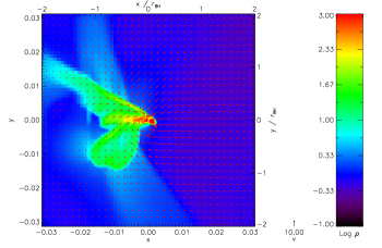
Figure 2.— Density (color) and velocity (arrows) around an accreting particle. The origin is centered on the accreting particle, and the axes show position in code units and in units of $r_{\rm BH}$.

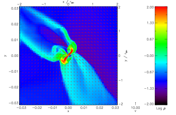
Figure 3.— Density (color) and velocity (arrows) around an accreting particle. The origin is centered on the accreting particle, and the axes show position in code units and in units of $r_{\rm BH}$.

We next compare the accretion rate predicted by our model to what we measure in the simulations. To measure the accretion rate in the simulations, we wait until $t>4t_{\rm BH}$, and compute the time-averaged accretion rate onto each particle thereafter. We then construct the cumulative distribution function of the accretion rates onto the particles, which we wish to compare with $P_{\dot{M}}(<\dot{M})$ as predicted by our models. For the model, we examine the simulation cube at the time when we insert the sink particles. We then compute $\dot{M}_{\rm BH}$ (equation 1 with $\lambda=\exp(1.5)/4$), $\dot{M}_{\omega}$ (equation 4) and $\dot{M}_{\rm turb}$ (equation 3) in every cell of the simulation. To measure vorticity, which is not a primitive of our simulation, we take two-sided differences over one cell at every point. From the grid of accretion rates, we compute $P_{\dot{M}}(<\dot{M})$, using $\dot{M}_{\rm BH}$, $\dot{M}_{\omega}$, and $\dot{M}_{\rm turb}$ in equation (8). We compare the predictions to the measured accretion rates in Figure 4.

Figure 4.— Cumulative (upper panel) and differential (lower panel) accretion rate PDFs vs. $\dot{M}/\dot{M}_{0}$. The curves shown are the measured value from the simulation (histogram) and the theoretical predictions using $\dot{M}_{\rm turb}$ (solid line), $\dot{M}_{\rm BH}$ (dashed line), and $\dot{M}_{\omega}$ (dotted line).

Note that, since $t_{\rm BH}\ll 1$, the state of the simulation cube on the large scale does not change much over the time after we insert the sink particles. For example, if we continue to let the box evolve without adding sink particles, after $4t_{\rm BH}$, the Mach number only decreases from $5.0$ to $4.7$. Thus, there is no problem in applying our simple model at the time just before we insert the sink particles. Also note that, at the time we measure vorticity, we have not yet inserted the sink particles and so there are no higher level AMR grids. When these grids first appear, the velocity is linearly interpolated on a cell-by-cell basis, so the vorticity in a refined cell is equal to that of its parent. However, as the simulation evolves, baroclinic instability generates vorticity structure on more refined levels just as it does on the base level. By the time our accretion rates stabilize, the vorticity structure on the more refined levels has had several crossing-times to reach equilibrium.

As Figure 4 shows, our ansatz function $\dot{M}_{\rm turb}$ gives excellent agreement with the simulation results. In contrast, using either $\dot{M}_{\rm BH}$ or $\dot{M}_{\omega}$ in place of $\dot{M}_{\rm turb}$ gives an extremely poor fit. We quantify this result by comparing the theoretical models to the simulations using a Kolmogorov-Smirnov (KS) test (Press et al., 1992). The KS statistic for our model is $0.81$. For the Padoan et al. (2005) proposal of using $\dot{M}_{\rm BH}$ where we use $\dot{M}_{\rm turb}$, it is $0.012$, and using $\dot{M}_{\omega}$ instead of $\dot{M}_{\rm turb}$ gives $2.7\times 10^{-10}$. This indicates that our model is highly consistent with the simulation data, while the two other candidates we have checked are essentially ruled out. The difference is large enough to have substantial astrophysical significance: the accretion rate averaged over particles that we measure in our simulations is $\langle\dot{M}\rangle/\dot{M}_{0}=0.73$, and our theory predicts a mean of $\langle\dot{M}\rangle/\dot{M}_{0}=0.90$. (The difference is larger than one might expect because our 64 particles do not sample the tail of the distribution very well.) In contrast, the Padoan et al. (2005) theory predicts $\langle\dot{M}\rangle/\dot{M}_{0}=4.3$, an ovestimate of nearly an order of magnitude.

Our theoretical model is well-described by a fit to a lognormal PDF. We find a best fit of

$$\frac{dp_{\dot{M}}}{d\ln\dot{M}}\approx 0.26\,\exp\left\{-\frac{\left[\ln\left(\dot{M}/\dot{M}_{0}\right)-1.1\right]^{2}}{2(1.6)^{2}}\right\}.$$ (15)

Figure 5 shows our fit in comparison to the simulation result.

Figure 5.— Numerical (solid line) and best-fit theoretical model (dashed line) accretion rate probability distributions vs. $\dot{M}/\dot{M}_{0}$.

A final question to consider is whether we might be underestimating the accretion rate because we only count mass that falls onto the particle, not mass that accumulates in the rotationally-supported torus or other bound structures around the particle. One might worry that these structures are acting as mass reservoirs, and that the accretion rate might rise at some point in the future as mass accretes from them on a viscous time scale. A priori this seems unlikely: Krumholz et al. (2005) simulate accretion with vorticity for 200 Bondi times and find that the rotationally-supported toruses do not act as reservoirs that raise the accretion rate at later times. Instead, the pattern is that the accretion rate starts high and gradually declines to its equilibrium value, while the toruses reach a steady mass, so that the ratio of torus mass to accreted mass declines steadily with time. Real accreting objects are likely to be in this limit where the torus mass is negligible compared to the total accreted mass. For example, the Bondi-Hoyle time for a protostar accreting in from a turbulent molecular clump is, as we show in § 5.3, only $\sim 10$ yr, vastly shorter than the time for which the protostar accretes.

We unfortunately cannot run our simulations for hundreds of Bondi-Hoyle times due to limitations of computational resources, and because over such long time scales the particles would likely interfere with one another. Thus, we cannot do a direct test as in Krumholz et al. (2005). However, to eliminate the possibility that we are missing substantial accretion by neglecting the gas in bound structures, we compute all the mass within a distance $r_{\rm BH}$ of each sink particle that has a potential energy larger than its kinetic energy, i.e. that is bound to that sink particle. We do this at $4t_{\rm BH}$, when the particle accretion rate has reached equilibrium, and at the final time in the simulation, roughly $4.4\,t_{\rm BH}$. We then compute the difference between the bound mass at $4t_{\rm BH}$ and at the final time. The median change in the mass of bound structures, divided by the median change in mass accreted onto particles over the same period, is 0.27. Thus, even if we were to assume that bound structures were reservoirs of mass that grow with time, the extra accretion onto them would only represent a $\sim 30\%$ correction to the accretion rate we have computed. If we add the accretion rate onto bound structures to the accretion rate onto particles, and compare that to our theoretical model using a KS test, we find a statistic of 0.15. While this is not quite as good as our value obtained using just the particles, this is still a reasonably good fit.

Note, however, that including the mass in bound structures only makes sense if they are truly accreting. Otherwise, adding their mass to the mass accreted by the particles is simply adding noise. It seems likely that this is the case, because the bound mass fluctuates strongly, and can be quite small compared to the accreted mass: for 16 of our 64 particles, the bound mass is less than 10% of the accreted mass at some point during the simulation, for 32 of the particles it is less than 25% of the accreted mass, and for 58 of them it is less than the accreted mass. Since the amount of mass that remains in the toruses over long times is small compared to the accreted mass, the toruses cannot be acting as mass reservoirs. Instead, the mass within them is transient, either on its way to being accreted or on its way out of the Bondi-Hoyle radius, not accumulating over a long term. Our estimates of the accretion rate using just the mass that falls onto the particles are more accurate.

4. The Accretion Rate in Turbulent Flows

Thus far we have shown that our model very accurately predicts the distribution of accretion rates in terms of the density and velocity field of the gas. We can use this result to derive an estimate for the accretion rate in a general turbulent flow in terms of a few simple parameters of the turbulent region that can usually be determined from observations. We consider a turbulent region of characteristic size $\ell$, mean density $\overline{\rho}$, sound speed $c_{\rm s}$, and three-dimensional Mach number $\mathcal{M}_{0}$, accreting onto an object of mass $M$. We derive a theoretical estimate for the mean and median accretion rate based on the probability distributions of density, velocity, and vorticity in a turbulent medium in § 4.1, and we compare it to simulations in § 4.2. We then discuss the issue of differences between mean and median accretion rates in § 4.3. In this Section we limit ourselves to discussing accretors randomly sampling turbulent regions. We discuss how to apply this results in real astrophysical situations in § 5.2 and § 5.3.

4.1. Theoretical Calculation

Although density, velocity, and vorticity in a turbulent medium are certainly correlated to some extent, that correlation is relatively weak. We can derive reasonable estimates for the functional dependence of the accretion rate on the properties of a turbulent region simply by neglecting correlations and assuming that density, velocity, and vorticity are selected independently from the appropriate PDF at every point.

Numerous authors have studied the PDF of densities in a turbulent medium (Vazquez-Semadeni, 1994; Padoan et al., 1997; Scalo et al., 1998; Passot & Vázquez-Semadeni, 1998; Nordlund & Padoan, 1999; Ostriker et al., 1999; Padoan & Nordlund, 2002). Padoan & Nordlund (2002) find that the PDF is well-fit by the functional form

$$\frac{dp_{\rho}(x)}{d\ln x}=\frac{1}{\sqrt{2\pi\sigma_{\rho}^{2}}}\exp\left[-\frac{\left(\ln x-\overline{\ln x}\right)^{2}}{2\sigma_{\rho}^{2}}\right]$$ (16)

where $x=\rho/\overline{\rho}$ is the density normalized to the mean density. The mean of the log of density (and also the log of the median density) is

$$\overline{\ln x}=-\frac{\sigma_{\rho}^{2}}{2}.$$ (17)

and the dispersion of the PDF is approximately

$$\sigma_{\rho}\approx\left[\ln\left(1+\frac{\mathcal{M}_{0}^{2}}{4}\right)\right]^{1/2},$$ (18)

The PDF of velocities is considerably less well-studied in the literature. Measuring from the simulations we describe in § 4.2, we find that the PDF is well-fit by a power law with an exponential cutoff,

$$\frac{dp_{v}(u)}{d\ln u}\propto u^{3}\exp\left(-1.5\,u^{1.7}\right),$$ (19)

where $u=v/(\mathcal{M}_{0}c_{\rm s})$ is the velocity normalized to the velocity dispersion of the region. Figure 6 shows our measurements from the simulations and our fit. The median velocity for this PDF is $1.2\,\mathcal{M}_{0}c_{\rm s}$, but the factor of 1.2 is relatively uncertain because it depends strongly on the form of the exponential cutoff, which is poorly constrained in our fit. We therefore simply take the median velocity to be $\mbox{median}(v)\equiv\phi_{\rm v}\mathcal{M}_{0}c_{\rm s}$, where $\phi_{\rm v}$ is a constant near unity.

Figure 6.— Measured values and fit for $dp_{v}(u)/d\ln u$. We show measurements from our 6 $N=256$ runs at $\mathcal{M}_{0}=3$ (diamonds), $\mathcal{M}_{0}=5$ (asterisks), and $\mathcal{M}_{0}=10$ (crosses), from our $N=512$ run at $\mathcal{M}_{0}=5$ (triangles), and our best fit (line).

The vorticity PDF is considerably more complex, as shown in Figure 7. In making the Figure we have introduced the normalized vorticity

$$\tilde{\omega}=\omega\frac{\ell}{\mathcal{M}_{0}c_{\rm s}},$$ (20)

which is related to the vorticity parameter for accretion onto an object by $\omega_{*}=\tilde{\omega}(\mathcal{M}_{0}r_{\rm B}/\ell)$. The vorticity PDF shows substantial variation from run to run, the shape does not appear to be independent of Mach number, and the shapes are not easily fit by a simple functional form. However, we can still obtain useful information by noting that the PDF peaks at roughly the same location independent of Mach number, and the median normalized vorticity is roughly constant. We estimate it as $\mbox{median}(\tilde{\omega})\equiv 10\,\phi_{\omega}$, where $\phi_{\omega}$ is a constant of order unity. Note that the fact that this peak is roughly independent of Mach number means that the median vorticity in a supersonically turbulent region is completely specified by its velocity dispersion and physical size.

Figure 7.— Measured values and estimated median for $dp_{\omega}(\tilde{\omega})/d\ln\tilde{\omega}$. We show measurements from our 6 $N=256$ runs at $\mathcal{M}_{0}=3$ (diamonds), $\mathcal{M}_{0}=5$ (asterisks), and $\mathcal{M}_{0}=10$ (crosses), and from our $N=512$ run at $\mathcal{M}_{0}=5$ (triangles).

From these PDFs, we can estimate the median accretion rate. Since we only expect the fit to be approximate, we simplify the results by setting $\lambda=1$ in equation (1) and by droping terms of order $\mathcal{M}_{0}^{-2}$ or smaller when added to terms of order unity. With these approximations, and neglecting correlations between density, velocity, and vorticity so that we can treat the median operator as linear, we predict that the median accretion rate, normalized to our simple Bondi-Hoyle estimate, will be

$$\phi_{\rm med} \equiv \mbox{median}(\dot{M})/\dot{M}_{0}$$ (21)

$$\approx \mbox{median}\left[\left(\dot{M}_{\rm BH}^{-2}+\dot{M}_{\omega}^{-2}\right)^{-1/2}\right]/\dot{M}_{0}$$ (22)

$$\approx \frac{\phi_{\rm v}^{-3}}{\sqrt{1+\mathcal{M}_{0}^{2}/4}}\left[1+\frac{10}{\phi_{\rm v}^{6}}\left(\frac{10\,\phi_{\omega}r_{\rm B}}{\ell\mathcal{M}_{0}^{2.3}}\right)^{1.8}\right]^{-0.5}.$$ (23)

The functional form agrees with what one would intuitively expect. When $r_{\rm B}/\ell$ is sufficiently small, vorticity has no effect on the accretion rate and all vorticity-related terms disappear. Instead, one is left with a median accretion rate that is close to the simple Bondi-Hoyle estimate $\dot{M}_{0}$. It is reduced relative to this, however, by the factor $(1+\mathcal{M}_{0}^{2}/4)^{-1/2}$, which is the ratio of the median to the mean density. When $r_{\rm B}/\ell$ is large enough that the term in square brackets is much greater than unity, the median accretion rate is controlled entirely by vorticity. Since the vorticity accretion rate depends approximately on $\omega_{*}^{-0.9}$, and $\omega_{*}\propto\phi_{\omega}r_{\rm B}/\ell$, we expect the accretion rate scale as $(\phi_{\omega}r_{\rm B}/\ell)^{-0.9}$, which is exactly what our estimate gives. The crossover between the two regimes occurs roughly when $\dot{M}_{\rm BH}=\dot{M}_{\omega}$, which occurs when the second term in the square brackets is about unity.

We can perform a similar procedure for the mean, although here we are considerably hampered by our uncertainties about the exact functional form of the vorticity and its dependence on Mach number. This uncertainty is amplified by the fact that the low vorticity tail of the PDF contributes significantly to the mean accretion rate. For this reason, we concentrate on estimating the mean accretion rate in the case where vorticity is irrelevant, and in § 4.2 we perform a purely empirical fit in the case where vorticity is important. For the case where vorticity is irrelevant, we compute the mean accretion rate by integrating over the density and velocity PDFs, again assuming that they are independent and setting $\lambda=1$ in (1). This gives

$$\phi_{\rm mean} \equiv \left\langle\dot{M}\right\rangle/\dot{M}_{0}$$ (24)

$$\approx \int_{0}^{\infty}\frac{1}{\left(\mathcal{M}_{0}^{-2}+u^{2}\right)^{3/2}}\frac{dp_{v}(u)}{du}\,du.$$ (25)

Although we can evaluate this expression numerically for our best-fit PDF, it is more convenient to approximate the integral in the case $\mathcal{M}_{0}\gg 1$ by treating the exponential cutoff in $dp_{v}(u)/du$ as a sharp truncation that gives unity at $u<\phi_{\rm u}$ and zero at $u>\phi_{\rm u}$, with $\phi_{\rm u}\approx 1$. The factor $\phi_{\rm u}$ represents our uncertainty in the exact shape of the exponential cutoff on the velocity PDF. With these approximations, we find

$$\phi_{\rm mean}\approx\frac{3}{\phi_{\rm u}^{3}}\left[\ln(2\phi_{\rm u}\mathcal{M}_{0})-1\right],\qquad\left(\frac{r_{\rm B}}{\ell}\rightarrow 0\right).$$ (26)

For $\phi_{\rm u}=1$, this expression agrees with (25) to better than $10\%$ for all Mach numbers between 2 and 200.

4.2. Comparison to Simulations

We now compare our theoretically predicted mean and median accretion rates to simulations. We run a series of simulations of periodic boxes, using the same methodology as described in § 3, and compute the mean and median values of the accretion rate using our simple model. To get a sense of the range of variation in accretion rates, we run six simulations at a resolution of $N=256$, each using a different random realization of the initial velocity field. We examine each run at the time when the Mach number has decayed to $\mathcal{M}_{0}=10$, $\mathcal{M}_{0}=5$, and finally $\mathcal{M}_{0}=3$. To compute the accretion rate from our simple model, we must also specify $r_{\rm B}/\ell$, the size of the particle’s Bondi radius relative to the size of the turbulent region, since the vorticity parameter $\omega_{*}$ is proportional to $r_{\rm B}$. We compute $\phi_{\rm mean}$ and $\phi_{\rm med}$ for each realization, at each Mach number, and a range of values of $r_{\rm B}/\ell$. Since our theory will probably fail for objects with Bondi-Hoyle radii comparable to the size of the entire turbulent region (see § 5.2), we limit ourselves to $r_{\rm BH}/\ell\raisebox{-2.15277pt}{$\>\stackrel{{\scriptstyle\textstyle<}}{{\sim}}\>$}0.1$, or $r_{\rm B}/\ell\raisebox{-2.15277pt}{$\>\stackrel{{\scriptstyle\textstyle<}}{{\sim}}\>$}10$ at $\mathcal{M}_{0}=10$.

We report the mean and standard deviation of the six runs, for selected values of $r_{\rm B}/\ell$, in Table 1, and plot the results in Figure 8. The Figure also shows fits based on our theoretical predictions for $\phi_{\rm med}$ and $\phi_{\rm mean}$. For $\phi_{\rm med}$, we find a good fit with equation (23) for $\phi_{\rm v}=0.93$ and $\phi_{\omega}=1.25$. For $\phi_{\rm mean}$, we only have a theoretical prediction for the low $r_{\rm B}/\ell$ case, so we fit to a function of the form $\phi_{\rm mean}=(\langle\dot{M}_{\rm BH}\rangle/\dot{M}_{0})[1+f(r_{\rm B}/\ell,\mathcal{M}_{0})]^{q}$, where $f(r_{\rm B}/\ell,\mathcal{M}_{0})$ is a power-law function of $r_{\rm B}/\ell$ and $\mathcal{M}_{0}$. We find that the function

$$\phi_{\rm mean}=\frac{3}{\phi_{\rm u}^{3}}\left[\ln(2\phi_{\rm u}\mathcal{M}_{0})-1\right]\left(1+100\frac{r_{\rm B}}{\ell\mathcal{M}_{0}}\right)^{-0.68}$$ (27)

with $\phi_{\rm u}=0.95$ fits the data reasonably well. Overall, we find that our predicted functional forms provide a good fit to the simulation data and capture the essential physics of the accretion process.

Table 1Selected computed accretion rates.

$\mathcal{M}_{0}$	$\log(r_{\rm B}/\ell)$	$\phi_{\rm mean}$	$\phi_{\rm med}$
3	$-5.0$	$2.2\pm 0.23$	$0.69\pm 0.14$
3	$-3.0$	$2.2\pm 0.22$	$0.69\pm 0.14$
3	$-1.0$	$0.93\pm 0.059$	$0.49\pm 0.092$
3	$1.0$	$0.038\pm 0.003$	$0.023\pm 0.003$
5	$-5.0$	$4.2\pm 0.34$	$0.42\pm 0.12$
5	$-3.0$	$4.0\pm 0.31$	$0.42\pm 0.12$
5	$-1.0$	$1.7\pm 0.072$	$0.39\pm 0.11$
5	$1.0$	$0.10\pm 0.004$	$0.047\pm 0.008$
10	$-5.0$	$7.9\pm 1.2$	$0.28\pm 0.074$
10	$-3.0$	$7.5\pm 1.1$	$0.28\pm 0.074$
10	$-1.0$	$3.7\pm 0.18$	$0.27\pm 0.071$
10	$1.0$	$0.40\pm 0.031$	$0.098\pm 0.016$

Note. — Cols. (3-4): Results are reported as $(\mbox{mean})\pm(\mbox{standard deviation})$.

Figure 8.— Measured and fit values of $\phi_{\rm mean}$ (upper panel) and $\phi_{\rm med}$ (lower panel) vs. $r_{\rm B}/\ell$. The plots show runs Mach 3 (diamonds), Mach 5 (asterisks), and Mach 10 (triangles), and our fits for these Mach numbers (solid lines). The error bars in the upper panel show the standard deviations in $\phi_{\rm mean}$. We do not show the error bars in $\phi_{\rm med}$ in the lower panel to avoid cluttering the plot.

Since the distribution of accretion rates is approximately lognormal, we can turn our fits for $\phi_{\rm mean}$ and $\phi_{\rm med}$ into fits for the entire PDF of accretion rates. A lognormal distribution is completely characterized by two parameters, the center of the distribution and its width, and we can solve for these in terms of $\phi_{\rm mean}$ and $\phi_{\rm med}$. Doing so, we find that the probability distribution of accretion rates in a turbulent medium is

$$\frac{dp_{\dot{M}}}{d\ln(\dot{M}/\dot{M}_{0})}=\frac{1}{\sqrt{2\pi\sigma_{\dot{M}}^{2}}}\cdot$$ (28)

$$\exp\left\{-\frac{\left[\ln(\dot{M}/\dot{M}_{0})-\overline{\ln(\dot{M}/\dot{M}_{0})}\right]^{2}}{2\sigma_{\dot{M}}^{2}}\right\},$$

where

$$\overline{\ln(\dot{M}/\dot{M}_{0})}=\ln\phi_{\rm med}$$ (29)

and

$$\sigma_{\dot{M}}=\sqrt{2\ln\frac{\phi_{\rm mean}}{\phi_{\rm med}}}.$$ (30)

4.3. Median versus Mean Accretion Rates

Since the volumetric median and mean accretion rates we have found can be quite different, we would like to determine whether one should use a median or a mean accretion rate in attempting to follow the evolution of an individual object. The mean and median are different because rare, high accretion regions contribute significantly to the overall accretion rate, even though it is very unlikely for a randomly placed accretor to be in one. When an object begins accreting in a turbulent medium, its accretion rate is most likely to be near the median. Over time, however, it will sample more and more of the turbulent medium, and its time-averaged accretion rate should approach the volume average for the region. We wish to determine how long this will take, since it is possible that it may be longer than the typical time that the object will spend in the turbulent region. This will tell us if our volumetric mean and median are truly good approximations for the mean and median accretion rate in time, measured for a single object rather than an ensemble.

To answer to the question of how long an object must accrete before reaching the volume mean accretion rate, we consider the related question of how far an object must move through a turbulent volume of gas before reaching the mean accretion rate. We answer this using the density and velocity field of our $N=512$ run at the point when $\mathcal{M}_{0}=5.0$, just before we insert the sink particles. The rate at which an accreting particle moves through the volume, accreting from new regions, should be roughly equal to the velocity dispersion of the gas. Thus, we place a particle at a random point within our turbulent box, moving in a random direction with velocity $\mathbf{v}$ such that $\left|\mathbf{v}\right|=5.0$, while the density and velocity of the gas remain fixed. We then compute the time-averaged accretion rate along the particle’s trajectory,

$$\left\langle\dot{M}\right\rangle=\frac{1}{T}\int_{0}^{T}\dot{M}_{\rm turb}(\mathbf{x}+\mathbf{v}t)\,dt,$$ (31)

as a function of time $T$. We repeat this procedure 1000 times. Figure 9 shows the fraction of particles for which the time-averaged accretion rate is closer to the volume-averaged mean than to the median as a function of time. (We use closer in a logarithmic sense, i.e. $\dot{m}>\sqrt{\phi_{\rm mean}\phi_{\rm med}}$.) The Figure also shows the fraction of particles whose time-averaged accretion rates are within a factor of 1.1 and within a factor of 2.0 of the mean accretion rate in the volume. A majority of the particles have time-averaged accretion rates closer to the mean than the median after only $0.25$ crossing times, where $t_{\rm cr}\equiv\ell/(\mathcal{M}_{0}c_{\rm s})=0.4$, but $95\%$ do not become closer to the mean than to the median until more than $6$ crossing times. Similarly, more than half of the particles are within a factor of $2.0$ of the mean accretion rate after only $0.28$ crossing times, but even after 10 crossing times fewer than half have time-averaged accretion rates within $10\%$ of the mean. Our conclusion is that one should use the mean rather than the median accretion rate to follow the evolution of any object that accretes for more than a quarter of a crossing time, but that one should not expect the time-averaged accretion rate to be closer than tens of percent to that value unless the particle accretes for a very long time.

Figure 9.— Fraction of particles vs. time. The curves show the fraction closer to the mean than the median (solid line), within a factor of $2.0$ of the mean accretion rate (dashed line), and within a factor of $1.1$ of the mean accretion rate (dot-dashed line).

5. Discussion

5.1. Resolution and Convergence

It is critical to establish that our simulations have sufficient resolution for us to believe our results. We first address whether we have enough resolution to compute the correct accretion rates onto our particles. Our simulation resolves the Bondi-Hoyle radius of the particles by 64 cells, and their Bondi radius by almost 1700 cells. Krumholz et al. (2004) found using the same code that we use here that in simulations of Bondi-Hoyle accretion a resolution of $\Delta x=r_{\rm BH}/50$ is more than adequate to reproduce the value found by previous theoretical and numerical work. Our resolution meets this requirement, although it is possible that for regions of the flow where the velocity is significantly higher than the mean we might not have sufficient resolution. At most this will affect the low accretion rate tail of the distribution, and should therefore not substantially bias our comparison between the accretion rate onto particles and our theoretical model. Similarly, Krumholz et al. (2005) found that $\Delta x=r_{\rm B}/160$ was sufficient to correctly model accretion with vorticity parameters up to $\omega_{*}=30$. The typical vorticity parameter we find in our simulation is somewhat greater than this, but by less than an order of magnitude. In contrast, our resolution is $\Delta x\approx r_{\rm B}/1700$, more than an order of magnitude greater than that Krumholz et al. (2005) found sufficient.

A related question is whether we have enough space between our particles for them to accrete independently of one another. A priori we do not expect the particles to interfere with one another, since they are separated by $32r_{\rm BH}$, much larger than any particle’s range of influence. There could potentially be interference between particles if one particle were upstream of another and significantly altered the flow of gas to its downstream neighbor. However, given the random alignment ot the turbulent flow, having one particle immediately upstream of another is extremeley unlikely. Even if one were upstream of another, we run the simulation for a time $\ll 32t_{\rm BH}$ once we insert the particles, so there is no time for depletion to propogate from one particle to another. Finally, we can find evidence against the possibility of interference between the particles by examining the accretion rates we actually measure. For Bondi-Hoyle accretion, the accretion rate depends on the accretion radius as $\dot{M}\propto r_{\rm acc}^{3/2}$, and a particle accreting at rate $\dot{M}_{0}$ has an accretion radius $r_{\rm acc}\approx r_{\rm BH}$. We would expect the particles to begin interfering with one another when the accretion radius is comparable to the half the inter-particle separation, or $16r_{\rm BH}$. This corresponds to an accretion rate of $64\dot{M}_{0}$. If interference between particles were a problem, we would expect to see the distribution of accretion rates truncated around $64\dot{M}_{0}$. However, Figure 4 shows that there are no particles accreting at anywhere near this rate, and that even our theoretical distribution predicts essentially no particles accreting at such high rates. We therefore conclude that none of our particles have accretion radii large enough for them to interfere with one another.

The final question of resolution is whether, before introducing our particles, we have enough resolution to model the turbulent flow field correctly. This question applies both to the $N=512$ run into which we insert our particles, and to the $N=256$ runs we use to estimate the mean and median accretion rates. To check convergence, we compare the distribution of accretion rates we find from the $N=256$ simulations at $\mathcal{M}_{0}=5.0$ to the $N=512$ run. We do this for $r_{\rm B}/\ell=0.20$, the value for our particles. Figure 10 shows the PDFs. The $N=512$ run mostly falls within the range of variation of the $N=256$ runs, although it is somewhat steeper, with less of the volume at high accretion rates. The average of the mean accretion rates in the $N=256$ runs is $1.26\,\dot{M}_{0}$, and the average of the medians is $0.36\,\dot{M}_{0}$. In comparison, for the $N=512$ run, the mean is $0.90\,\dot{M}_{0}$, and the median is $0.34\,\dot{M}_{0}$. The agreement on the medians is very good, and well within the variation among the $N=256$ runs, but the agreement on the means is only fair. The difference in quality of convergence probably occurs because the medians are sensitive to the peak of the distribution, but the means depend more on the low vorticity, high accretion rate tail of the distribution that is more sensitive to resolution. Thus, our means probably have a $\sim 25\%$ systematic error.

Figure 10.— PDF of accretion rates for the $N=256$ runs (dashed lines) and the $N=512$ run (solid line).

As a final note, the behavior of vorticity with resolution is interesting, and helps explain why we are better converged in the median than in the mean accretion rate and why the mean is decreasing with resolution. We compute the mean and median vorticity in the velocity field of our $N=512$ run when $\mathcal{M}_{0}=5.0$, just before we insert the sink particles. We then sample the simulation down to $N=256$, $N=128$, $N=64$, and $N=32$ and compute the mean and median vorticity for those resolutions. Both the mean and median vorticity increase monotonically with $N$, but the median vorticity appears to be converging while the mean only shows slight curvature and may actually be diverging. We show this in Figure 11. The mean is controlled by a high vorticity tail, and it appears likely that there is no converged value for it until one reaches the dissipation scale, either due to grid viscosity (in a simulation) or due to physical viscosity (in a real fluid). In contrast, the median appears to be well-defined and converged at $N=512$; the difference in median between the $N=256$ and $N=512$ resolutions is less than $2\%$, and the median vorticity is rising with $N$ only as $N^{0.026}$. A similar trend is visible in Figure 7, where the $N=512$ run peaks at roughly the same location as the $N=256$ runs, but has a longer high-vorticity tail.

The divergence of the mean does not affect the convergence of our results, however. The high vorticity tail that causes the mean vorticity to diverge corresponds to low accretion rates. Thus, it will not cause the mean accretion rate to diverge. Nor will it cause our accretion rate to go to zero as resolution increases. The high vorticity tail will simply contribute less and less to the mean accretion rate as the resolution increases, but the contribution from vorticities near the median will not decrease because the median does not change with resolution. Thus, we can regard our $\sim 25\%$ change between the $N=256$ and $N=512$ runs as a rough estimate of the likely error from imperfect convergence. However, we conjecture that vorticity on scales much smaller than $r_{\rm BH}$ will not significantly affect the accretion rate. In our $N=512$ runs, we have $r_{\rm BH}/\Delta x=4$ on the base AMR level. (Once we insert the particles we greatly increase the resolution around them, but our estimates of $\phi_{\rm mean}$ are based on the simulation cube before that insertion). Since we already have marginal resolution at $N=512$, we believe it is unlikely that increasing resolution past $N=512$ will stronlgy affect $\phi_{\rm mean}$. Also note that this convergence issue only affects accretion when $r_{\rm B}/\ell$ is large enough to affect the accretion rate. The velocity PDFs, as shown in Figure 6, are already very well converged at $N=256$, so only when vorticity becomes important are our results uncertain.

Figure 11.— Mean (upper line) and median (lower line) normalized vorticity $\tilde{\omega}$ versus resolution.

5.2. Limitations

There are several limitations to our results. First, we have neglected magnetic fields. These are likely to suppress the accretion rate relative to what we have found, because they will restrict the flow of gas across magnetic field lines to an accreting object. In molecular clouds, where the Alfvén Mach number is of order unity (McKee, 1989; McKee et al., 1993; Crutcher, 1999) or less (Padoan et al., 2004), the effect is likely to be of order unity. However, magnetohydrodynamic simulations similar to the ones we have performed will be required to make a more definitive statement. A related limitation is that we have not considered a self-gravitating medium. If the gas is strongly self-gravitating, its density and velocity distributions will change, and our results for $\phi_{\rm mean}$ and $\phi_{\rm med}$ may need to be modified. However, our central result that vorticity is critical in setting the accretion rate will not be affected by the addition of self-gravity.

A second limitation is that our approach is likely to break down for subsonic turbulence. The distribution of densities and velocities is different in subsonically turbulent media than in supersonically turbulent ones, so our results will not extrapolate to that regime. For very subsonic turbulence where there is some vorticity present, it is likely that the accretion flow approaches the vorticity-dominated low $\omega_{*}$ regime identified by Krumholz et al. (2005). The transition should occur for values of $\mathcal{M}_{0}$ near unity. However, we have not mapped out the details of the change from one regime to the other, so we must be careful in attempting to apply our theory to the warm atomic or ionized phases of the ISM, since the motions in these phases are generally transsonic or subsonic.

Third, our results are only applicable to objects with Bondi-Hoyle radii significantly smaller than the size of the turbulent gas cloud in which they are accreting. Our estimate of the accretion rate is based on the assumption that, on large scales, the turbulent gas is uniform and can be roughly modeled by a periodic box. However, if $r_{\rm BH}\raisebox{-2.15277pt}{$\>\stackrel{{\scriptstyle\textstyle>}}{{\sim}}\>$}\ell$, then the turbulent gas will become centrally condensed due the gravity of the accretor, and our assumption of uniformity will fail.

The final major limitation is that we have only considered the case in which the accreting object is not moving through the turbulent medium at a velocity comparable to or larger than the velocity dispersion of the gas. In such a situation an accretor should undergo velocity-dominated accretion regardless of its position in the turbulent medium. The accretion rate will be the standard Bondi-Hoyle rate, using the local density as $\rho_{\infty}$. Consequently, the distribution of accretion rates should be proportional to the distribution of densities, which is well measured from simulations (e.g. Padoan & Nordlund, 1999). This limitation prevents us from applying our theory to neutron stars or black holes passing through molecular clouds, since these objects generally have velocity much larger than the turbulent velocity dispersions of GMCs.

One might think that our assumption of isothermality also presents a considerable limitation. However, this is not likely to be the case. In ordinary Bondi-Hoyle accretion, changing the equation of state only changes the accretion rate by factors of order unity (Ruffert, 1994; Ruffert & Arnett, 1994). Thus, a different equation of state is not likely to change the nature of the accretion flow onto a particle. The only way that a change in the equation of state might affect our accretion rates is by changing the distribution of densities, velocities, and vorticities in the turbulent gas. Since we are assuming the turbulence is highly supersonic, a different equation of state is unlikely to affect the velocity field very much; thermal energy will always be considerably less than kinetic energy over most of the flow. The remaining potential effect of non-isothermality is on the density field. Passot & Vázquez-Semadeni (1998) show that isothermal turbulence leads to a PDF of densities that is lognormal. Polytropic indices $\gamma<1$ lead the PDF to develop a power-law tail at high densities, and indices $\gamma>1$ lead to a power-law tail at low densities. The latter is unlikely to affect the accretion rate, since the low density gas that is affected does not contribute significantly to the mean or median accretion rate. If $\gamma<1$, there will be more gas at high densities than in the isothermal case, and the accretion rate is likely to be larger than we have estimated by an amount that depends on how small $\gamma$ is. Our results are therefore likely to change only by order unity for $\gamma>1$, and will only change by much more than that if $\gamma\ll 1$.

5.3. Implications

Our results have implications for several astrophysical problems. Here we sketch out three. The first is the problem of pre-main sequence accretion. Padoan et al. (2005) consider accretion onto T Tauri stars from a turbulent medium using the ansatz $\dot{M}_{\rm turb}=\dot{M}_{\rm BH}$. (Note that this is slow accretion that takes place after the pre-stellar core has collapsed and been accreted, not the competitive accretion model of star formation. We discuss competitive accretion below.) They find an accretion rate consistent with observed accretion rates onto pre-main sequence stars and brown dwarfs in nearby low-mass star-forming regions. We have shown that using $\dot{M}_{\rm turb}=\dot{M}_{\rm BH}$ can lead to significant overestimates of the accretion rate, and that the mean and median accretion rate are quite different. Accretion rates are inferred from observations of the accretion luminosity, which is sensitive to the accretion rate on time scales far smaller than the crossing time of the system. Thus, one should use the median rather than the mean accretion rate when comparing to individual accreting objects. However, we find that Padoan et al.’s conclusions are not affected too strongly by our results, provided their application is limited to the low-mass star-forming regions to which Padoan et al. compare their models. Such regions have widely distributed pre-main sequence stars and star-forming clumps with large radii. If stars are forming in a turbulent clump of size $\ell\sim 5$ pc, as Padoan et al. assume, then for a 1 $M_{\odot}$ star $r_{\rm B}/\ell\approx 0.02$ (for 10 K gas), and vorticity is relatively unimportant.

On the other hand, massive star-forming regions are more compact and turbulent, and star-forming clumps there are more typically on scales $\ell\approx 0.5$ pc, with Mach numbers $\mathcal{M}_{0}\sim 20$ (Plume et al., 1997). Levels of turbulence are not significantly lower in starless cores, so it is likely that these Mach numbers are typical even at early stages of the star formation process (Yonekura et al., 2005). For such a region $r_{\rm B}/\ell\approx 0.2$ for a 1 $M_{\odot}$ star, and vorticity can suppress accretion. This conclusion leads to the possibility of an interesting observational test of our conclusions. Assuming that Padoan et al. are correct and that accretion onto protostars comes primarily from accretion of gas from the environment (rather than from some internal process involving an accretion disk), one could bin accreting stars by mass, and look for a change in the dispersion of accretion rates versus mass. This break should occur because the mean and median accretion rate begin to be affected by vorticity at different values of $r_{\rm B}/\ell$. Using (27), in a clump with $\mathcal{M}_{0}=20$, $\phi_{\rm mean}$ is independent of mass for stars of mass $M<1$ $M_{\odot}$, and $\phi_{\rm mean}\propto M^{-0.7}$ for more massive stars. On the other hand, $\phi_{\rm med}$ is independent of mass up to a mass of $130$ $M_{\odot}$, vastly larger than any observed protostar. Thus, above $1$ $M_{\odot}$ the ratio $\phi_{\rm mean}/\phi_{\rm med}\propto M^{-0.7}$, and the dispersion of accretion rates, which depends on this ratio, should decrease with mass. Given a reasonably large sample of accreting protostars in a dense clump with a range of masses above and below $1$ $M_{\odot}$, one could see this decrease in dispersion with mass. One could also in principle look for the change in $\phi_{\rm mean}$ with mass directly, but this is more difficult because one would need a very large sample of accreting stars to determine $\phi_{\rm mean}$ accurately. Measuring the dispersion requires fewer sources. Even so, measuring accretion luminosities of T Tauri stars in massive star forming regions is a significant observational challenge due to distance, confusion, and extinction. Unfortunately one cannot test our model using more massive stars, because the rate of Bondi-Hoyle accretion onto stars larger than $\sim 10$ $M_{\odot}$ is likely to be substantially reduced by radiaton pressure (Edgar & Clarke, 2004).

A second potential implication is in the area of competitive accretion. In this model of star formation, the initial mass function is determined by seed protostars accreting unbound gas within the turbulent molecular clump where they form (e.g. Bonnell et al., 1997; Klessen & Burkert, 2000, 2001; Bonnell et al., 2001a, b, 2004). Our theory does not apply during the first stage of competitive accretion, when a star is still accreting from its initial bound core, for two reasons. First, the core is bound to the star and to itself, while we have considered accretion of unbound gas. Second, the star is co-moving with the gas in its core, so it is not randomly sampling the turbulent flow. Once the star accretes its parent core, these limits no longer apply and one may use our theory. The star is no longer accreting bound gas, and, since the time required to accrete the bound core (which is comparable to the dynamical time of the parent clump – McKee & Tan, 2003) will allow the star to become dynamically decoupled from the turbulent flow, the star will be randomly sampling the gas in the molecular clump to which it is gravitationally confined.

Our results suggest that in this stage the accretion rate in such clumps may be considerably different than a naive application of the Bondi-Hoyle formula suggests. Simulations of competitive accretion performed to date likely have too little resolution to accurately model the effect we describe here. In a typical massive star-forming clump, the velocity dispersion is $\sim 4$ km s^-1 (Plume et al., 1997; Yonekura et al., 2005), giving a Bondi-Hoyle radius for a $0.1$ $M_{\odot}$ seed protostar of only 5.5 AU, far smaller than the resolution of the simulations performed thus far. Published calculations of competitive accretion to date have largely avoided the problem by using the lower velocity dispersions characteristic of low-mass star forming regions. However, it represents a formidable obstacle to simulating the formation of rich clusters from massive clumps. It is unclear what effect failing to resolve this radius would have on the computed accretion rate. Competitive accretion simulations generally use smoothed-particle hydrodynamics with sink particles, and these methods compare the kinetic and potential energies of a gas particle in an attempt to determine whether it is bound to a sink particle before accreting it (Bate et al., 1995). As a result, the most likely error is an understimate of the accretion rate caused by failure to resolve the Bondi-Hoyle accretion shock cone and the resulting loss of gas kinetic energy.

A third potential implication of our result is for the accretion rates of black holes in the centers of galaxies. Some simulations and semi-analytic models of the growth of galactic center BHs assume that the black holes accrete at the Bondi rate (e.g. Springel et al., 2005). If the gas around the black hole is turbulent, however, using the Bondi rate may lead to significant errors. It is uncertain whether the accretion process onto galactic center BHs can be described by Bondi accretion at all, but, if it can, then simulations and analytic models should use the turbulent accretion rate we have found rather than the unmodified Bondi rate.

6. Conclusions

The primary result of our investigation is that the accretion rate in a turbulent medium is significantly enhanced over the zeroth-order estimate one obtains by simply using the turbulent velocity dispersion in the Bondi-Hoyle formula. However, this enhancement may be partially or completely offset by the effects of vorticity within the turbulent medium, and may even be suppressed below the Bondi-Hoyle rate for Mach numbers near or below unity. For this reason, simply using the Bondi-Hoyle formula either by treating the global velocity dispersion as a sound speed or by applying the formula to every point within the medium (Padoan et al., 2005) does not produce the correct accretion rate. On the other hand, approximating the accretion process as being dominated by either velocity or vorticity, and using the lesser of the two implied accretion rates, appears very consistent with the results of simulations.

We use this simple model to compute the probability distribution of accretion rates onto point particles in a turbulent medium. The PDF of accretion rates is lognormal, and we give simple formulae that specify the shape of the lognormal distribution, and the mean and median accretion rates, over a relatively wide range of accretor masses and turbulent Mach numbers. The mean and median accretion rates can be quite different, due to the long tail of the lognormal accretion rate distribution, and it takes an accreting particle of order a crossing time of the turbulent region before its time-averaged accretion rate approaches the mean for the region.

Our findings suggest that a number of previously published numerical and analytical results may need to be reconsidered, and that future work may have to meet quite severe resolution constraints. Estimates of accretion rates in star-forming regions using the simple Bondi-Hoyle formula are probably incorrect, and simulations of competitive accretion that do not resolve the Bondi-Hoyle radius, and possibly even smaller scales, are likely to produce incorrect accretion rates. Simulations of star formation that have been completed to date have largely avoided this problem by not simulating the very large velocity dispersions found in massive star-forming regions, and our work shows that expanding the simulations to these regions will require much higher resolution. We leave a more detailed reconsideration of these problems, using our newly developed theory of Bondi-Hoyle accretion in a turbulent medium, to future work.

References

- Abramowicz & Zurek (1981) Abramowicz, M. A. & Zurek, W. H. 1981, ApJ, 246, 314
- Bate et al. (1995) Bate, M. R., Bonnell, I. A., & Price, N. M. 1995, MNRAS, 277, 362
- Bell et al. (1984) Bell, J., Berger, M. J., Saltzman, J., & Welcome, M. 1984, SIAM J. Sci. Comp., 15, 127
- Berger & Collela (1989) Berger, M. J. & Collela, P. 1989, J. Comp. Phys., 82, 64
- Berger & Oliger (1984) Berger, M. J. & Oliger, J. 1984, J. Comp. Phys., 53, 484
- Bondi (1952) Bondi, H. 1952, MNRAS, 112, 195
- Bonnell et al. (1997) Bonnell, I. A., Bate, M. R., Clarke, C. J., & Pringle, J. E. 1997, MNRAS, 285, 201
- Bonnell et al. (2001a) —. 2001a, MNRAS, 323, 785
- Bonnell et al. (2001b) Bonnell, I. A., Clarke, C. J., Bate, M. R., & Pringle, J. E. 2001b, MNRAS, 324, 573
- Bonnell et al. (2004) Bonnell, I. A., Vine, S. G., & Bate, M. R. 2004, MNRAS, 349, 735
- Crutcher (1999) Crutcher, R. M. 1999, ApJ, 520, 706
- Dubinski et al. (1995) Dubinski, J., Narayan, R., & Phillips, T. G. 1995, ApJ, 448, 226
- Edgar & Clarke (2004) Edgar, R. & Clarke, C. 2004, MNRAS, 349, 678
- Foglizzo & Ruffert (1999) Foglizzo, T. & Ruffert, M. 1999, A&A, 347, 901
- Fryxell & Taam (1988) Fryxell, B. A. & Taam, R. E. 1988, ApJ, 335, 862
- Hoyle & Lyttleton (1939) Hoyle, F. & Lyttleton, R. A. 1939, in Proceedings of the Cambridge Philisophical Society, 405–+
- Igumenshchev & Abramowicz (2000) Igumenshchev, I. V. & Abramowicz, M. A. 2000, ApJS, 130, 463
- Igumenshchev et al. (2000) Igumenshchev, I. V., Abramowicz, M. A., & Narayan, R. 2000, ApJ, 537, L27
- Klein (1999) Klein, R. I. 1999, J. Comp. App. Math., 109, 123
- Klessen & Burkert (2000) Klessen, R. S. & Burkert, A. 2000, ApJS, 128, 287
- Klessen & Burkert (2001) —. 2001, ApJ, 549, 386
- Krumholz et al. (2004) Krumholz, M. R., McKee, C. F., & Klein, R. I. 2004, ApJ, 611, 399
- Krumholz et al. (2005) —. 2005, ApJ, 618, 757
- McKee (1989) McKee, C. F. 1989, ApJ, 345, 782
- McKee & Tan (2003) McKee, C. F. & Tan, J. C. 2003, ApJ, 585, 850
- McKee et al. (1993) McKee, C. F., Zweibel, E. G., Goodman, A. A., & Heiles, C. 1993, in Protostars and Planets III, 327–+
- Nordlund & Padoan (1999) Nordlund, Å. K. & Padoan, P. 1999, in Interstellar Turbulence, 218–+
- Ostriker et al. (1999) Ostriker, E. C., Gammie, C. F., & Stone, J. M. 1999, ApJ, 513, 259
- Padoan et al. (2004) Padoan, P., Jimenez, R., Juvela, M., & Nordlund, Å. 2004, ApJ, 604, L49
- Padoan et al. (2005) Padoan, P., Kritsuk, A., Norman, M. L., & Nordlund, Å. 2005, ApJ, 622, L61
- Padoan & Nordlund (1999) Padoan, P. & Nordlund, Å. 1999, ApJ, 526, 279
- Padoan & Nordlund (2002) —. 2002, ApJ, 576, 870
- Padoan et al. (1997) Padoan, P., Nordlund, A., & Jones, B. J. T. 1997, MNRAS, 288, 145
- Passot & Vázquez-Semadeni (1998) Passot, T. & Vázquez-Semadeni, E. 1998, Phys. Rev. E, 58, 4501
- Plume et al. (1997) Plume, R., Jaffe, D. T., Evans, N. J., Martin-Pintado, J., & Gomez-Gonzalez, J. 1997, ApJ, 476, 730
- Press et al. (1992) Press, W. H., Teukolsky, S. A., Vetterling, W. T., & Flannery, B. P. 1992, Numerical Recipes in C, 2nd Edition (New York: Cambridge University Press)
- Proga & Begelman (2003) Proga, D. & Begelman, M. C. 2003, ApJ, 582, 69
- Ruffert (1994) Ruffert, M. 1994, ApJ, 427, 342
- Ruffert (1997) —. 1997, A&A, 317, 793
- Ruffert (1999) —. 1999, A&A, 346, 861
- Ruffert & Arnett (1994) Ruffert, M. & Arnett, D. 1994, ApJ, 427, 351
- Scalo et al. (1998) Scalo, J., Vazquez-Semadeni, E., Chappell, D., & Passot, T. 1998, ApJ, 504, 835
- Sparke (1982) Sparke, L. S. 1982, ApJ, 254, 456
- Sparke & Shu (1980) Sparke, L. S. & Shu, F. H. 1980, ApJ, 241, L65
- Springel et al. (2005) Springel, V., Di Matteo, T., & Hernquist, L. 2005, MNRAS, 623
- Toro (1997) Toro, E. 1997, Riemann Solvers and Numerical Methods for Fluid Dynamics: A Practical Introduction (Berlin: Springer)
- Truelove et al. (1998) Truelove, J. K., Klein, R. I., McKee, C. F., Holliman, J. H., Howell, L. H., Greenough, J. A., & Woods, D. T. 1998, ApJ, 495, 821
- Vazquez-Semadeni (1994) Vazquez-Semadeni, E. 1994, ApJ, 423, 681
- Vazquez-Semadeni et al. (2000) Vazquez-Semadeni, E., Ostriker, E. C., Passot, T., Gammie, C. F., & Stone, J. M. 2000, Protostars and Planets IV, 3
- Yonekura et al. (2005) Yonekura, Y., Asayam, S., Kimura, K., Ogawa, H., Kanai, Y., Yamaguchi, N., Fukui, Y., & Barnes, P. J. 2005, ApJ, in press, astro-ph/0508121