Ly$\alpha$ Radiation From Collapsing Protogalaxies II:
Observational Evidence for Gas Infall.

Abstract

We model the spectra and surface brightness distributions for the Ly$\alpha$ radiation expected from protogalaxies that are caught in the early stages of their assembly. We use the results of a companion paper to characterize the radiation emerging from spherically collapsing gas clouds. We then modify these spectra to incorporate the effect of subsequent resonant scattering in the intergalactic medium (IGM). Using these models, we interpret a number of recent observations of extended Ly$\alpha$ blobs (LABs) at high redshift. We suggest, based on the angular size, energetics, as well as the relatively shallow surface brightness profiles, and double-peaked spectra, that several of these LABs may be associated with collapsing protogalaxies. We suggest two follow-up observations to diagnose the presence of gas infall. High S/N spectra of LABs should reveal a preferential flattening of the surface brightness profile at the red side of the line. Complementary imaging of the blobs at redshifted H$\alpha$ wavelengths should reveal the intrinsic Ly$\alpha$ emissivity and allow its separation from radiative transfer effects. We show that Ly$\alpha$ scattering by infalling gas can reproduce the observed spectrum of Steidel et al’s LAB2 as accurately as a recently proposed outflow model. Finally, we find similar evidence for infall in the spectra of point–like Ly$\alpha$ emitters. The presence of scattering by the infalling gas implies that the intrinsic Ly$\alpha$ luminosities, and derived quantities, such as the star–formation rate, in these objects may have been underestimated by about an order of magnitude.

1 Introduction

Copious Ly$\alpha$ emission may be associated with the early stages of the formation of galaxies. The epoch before the onset of significant star formation in the history of an individual galaxy, hereafter referred to as the ‘protogalactic’ stage, may be accompanied by the release of the gravitational binding energy through Ly$\alpha$ cooling radiation (Haiman et al., 2000; Fardal et al., 2001). The extended Ly$\alpha$ “fuzz” surrounding these protogalaxies may be strongly enhanced in the presence of a central ionizing source, such as a quasar (Haiman & Rees, 2001; Haiman, 2004), as evidenced by a handful of recent observations (Bunker et al., 2003a; Weidinger et al., 2004, 2005; Christensen et al., 2006). As the number of known high redshift Ly$\alpha$ emitters, both point–like (e.g. Rhoads et al., 2000; Rhoads & Malhotra, 2001; Ajiki et al., 2003; Kodaira, 2003; Hu et al., 2004; Rhoads et al., 2004; Ouchi, 2005) and extended (e.g Steidel et al., 2000; Matsuda, 2004; Wilman et al., 2005; Dey et al., 2005; Nilsson et al., 2005; Matsuda et al., 2006) grows, there is an increasing need for diagnosing the presence of any large–scale gas infall.

In Dijkstra et al. (2006, hereafter paper I) we presented Monte Carlo simulations of the transfer of Ly$\alpha$ photons through spherically symmetric models of neutral collapsing gas clouds. These models are intended as simplified descriptions of protogalaxies in the process of their assembly. We computed the spectra and surface brightness profiles emerging from clouds with a range of properties. For clouds without any associated ionizing source, generating Ly$\alpha$ photons through cooling radiation alone, we explored two extreme models. In the ‘extended models’, the gas continuously emits a significant fraction of its gravitational binding energy in the Ly$\alpha$ line as it navigates down the dark matter potential well. In the “central” models, Ly$\alpha\hskip 2.84526pt$photons are generated only at the center of the collapsing cloud. We then studied how the results of these calculations were affected by the presence of a central ionizing source. The main results that are relevant to the present paper can be summarized as follows:

(i) In the absence of an ionizing source (i.e. stars or a quasar) the emergent Ly$\alpha$ spectrum is typically double–peaked and asymmetric. Transfer of energy from the collapsing gas to the Ly$\alpha$ photons -together with a reduced escape probability for photons in the red wing- causes the blue peak to be significantly enhanced, which results in an effective blueshift of the Ly$\alpha$ line. This blueshift may easily be as large as $\sim 2000$ km s^-1. The total blueshift of the line increases with the total column density of neutral hydrogen of the gas and with its infall speed. The prominence of the red peak is enhanced towards higher redshift, lower mass and lower infall speeds. If detected, the shift of the red peak relative to the line center potentially measures the gas infall speed.

(ii) In the “central” models, the Ly$\alpha$ radiation emerges with a steeper surface brightness profile, and with a larger blueshift, than in the “extended” models.

(iii) A steepening of the surface brightness distribution towards bluer wavelengths within the Ly$\alpha$ line is indicative of gas infall.

(iv) In clouds that are fully ionized by an embedded ionizing source, the effective Ly$\alpha$ optical depth is reduced typically to $\;\hbox to0.0pt{\lower 2.5pt\hbox{$\sim$}\hss}\raise 1.5pt\hbox{$<$}\;10^{3}$. In these cases, the Ly$\alpha$ emission emerges with a nearly symmetric profile, and its FWHM is determined solely by the bulk velocity field of the gas. Its overall blueshift is reduced significantly (and may vanish completely for very bright ionizing sources). As a result, infall and outflow models can produce nearly identical spectra and surface brightness distributions, and are difficult to distinguish from one another.

For a detailed description of several other features of the emergent Ly$\alpha$ radiation the reader is referred to paper I. The models discussed in paper I are oversimplified, for a discussion on the uncertainties this may introduce the reader is referred to paper I, specifically section 8.2. The results presented in paper I generally ignored the transfer through the intergalactic medium (IGM). Since the IGM is optically thick at the Ly$\alpha$ frequency at $z\;\hbox to0.0pt{\lower 2.5pt\hbox{$\sim$}\hss}\raise 1.5pt\hbox{$>$}\;3$, to allow comparison of these results with the observations, the scattering of Ly$\alpha$ photons through the IGM needs to be modeled. Note that we define the IGM to commence beyond the virial radius of an object. The intrinsic spectrum refers to the spectrum as it emerges at the virial radius. In the present paper, we adopt a simple model of the IGM gas density and velocity distribution expected near protogalaxies, based on the models of Barkana (2004). Combining the results obtained in paper I with the scattering in the IGM, we compare our models to several observations in the literature. We focus on interpreting those extended Ly$\alpha$ blobs (LABs) that have no continuum source, or surround a radio quiet quasar. While LABs are known to exist around radio loud quasars, they are attributable to known jets and supernova–driven outflows, and we do not attempt to model them here (e.g. Hu et al., 1991; Wilman et al., 2000). We also compare our results with the recently discovered high redshift ($z>5$) Ly$\alpha$ emitters, which generally appear point–like. Despite the over–simplified nature of our model of the protogalactic gas and the IGM, we successfully reproduce several observed Ly$\alpha$ spectral features.

The rest of this paper is organized as follows. In § 2, we describe our model of the IGM and discuss its impact on our results from paper I. In § 3, we compare our model predictions with the properties of several known high–redshift Ly$\alpha$ emitting sources. In § 4, we discuss our results and their cosmological relevance. We also discuss the possibility of imaging the protogalaxies in the H$\alpha$. Since this line should not suffer from attenuation in the IGM, it may have a surface brightness comparable to (or even exceeding) that of the Ly$\alpha$ line. Finally, in § 5, we present our conclusions and summarize the implications of this work. The parameters for the background cosmology used throughout this paper are $\Omega_{m}=0.3$, $\Omega_{\Lambda}=0.7$, $\Omega_{b}=0.044$, $h=0.7$, based on Spergel et al. (2003).

2 The Impact of the IGM

2.1 Impact of a Static IGM

In the simplest model, employed occasionally in paper I, Ly$\alpha$ photons are injected into a statistically uniform IGM, following Hubble expansion. Photons with an original wavelength blueward of the Ly$\alpha$ line center redshift into resonance and may get scattered out of our line of sight. Ly$\alpha$ photons that are initially redward of the line center are not scattered resonantly (scattering in the red damping wing is not important in the present context, at redshifts at which the IGM is highly ionized). We follow paper I and define $x$ as a dimensionless frequency variable, which measures the offset from the line center in units of the Doppler width, $x\equiv(\nu-\nu_{0})/\Delta\nu_{D}$. Note that positive/negative values of $x$ correspond to blueshifted/redshifted Ly$\alpha$ photons. The IGM then allows a transmission of a fraction $\langle\exp{(-\tau)}\rangle$ and $1$ with $x>0$ and $x\leq 0$ of photons emerging from the collapsing cloud, respectively. Here, $\langle\exp{(-\tau)}\rangle$ denotes the mean IGM transmission as it has been determined observationally in studies of the Ly$\alpha$ forest. Table 1 shows $\langle\exp{(-\tau)}\rangle$ as a function of redshift. The second row shows $\sigma_{f}$, which is the reported measurement error ($1-\sigma$) in $f$. This Table shows that attenuation by the IGM is significant at $z\;\hbox to0.0pt{\lower 2.5pt\hbox{$\sim$}\hss}\raise 1.5pt\hbox{$>$}\;3$.

Table 1: Transmission of IGM

z	2.4	3.0	3.8	4.5	5.2	5.7	6.0
$f\equiv\langle\exp{(-\tau)}\rangle$	0.8	0.68	0.49	0.25	0.09	0.07	0.004
$\sigma_{f}$					0.02	0.003	0.003
(1) From McDonald et al. (2001)
(2) From Songaila & Cowie (2002); Fan et al. (2002)

2.2 Impact of a Dynamic IGM

Protogalaxies are likely to reside in relatively massive halos, corresponding to high–$\sigma$ density peaks in the IGM. The gravitational field of the halos causes material on large scales to decouple from the Hubble flow and fall in toward the halo. Barkana (2004) has modelled the density and velocity distribution of the IGM around nonlinear halos. In these models, around the massive halos typically considered in paper I, infall may occur up to about $\sim 5$ virial radii. Photons that escape the protogalaxy with a small redshift, $x\;\hbox to0.0pt{\lower 2.5pt\hbox{$\sim$}\hss}\raise 1.5pt\hbox{$<$}\;0$, may then be resonantly scattered by the infalling gas. As a result, significant attenuation can extend into the red part of the observed spectrum. To give a quantitative example (see Figure 2 and 4 in Barkana 2004), for a dark matter halo with a total mass of $10^{12}~{}{\rm M_{\odot}}$, the overdensity of the IGM is expected to be $\delta\sim 20-30$ at the virial radius, and still $\delta\sim 2-3$ at $\sim 10$ virial radii from the object. The infall velocity is equal to the circular velocity at the virial radius. The IGM is at rest with respect to the virialized object approximately 5 virial radii away. The radius at which the peculiar velocity of the IGM vanishes (and is therefore comoving with the Hubble flow ) is further out, and is mass dependent.

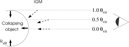
Figure 1: This drawing illustrates the effect of the impact parameter on the IGM transmission. The IGM is assumed to undergo spherically symmetric infall. In this case, photons emerging from the edge of our object (in the direction along the line of sight) see a projected version of the IGM velocity field.

The impact of the IGM will be further modified by the proximity effect near bright QSOs. For bright QSOs, the size of the local HII region can extend beyond $\sim 5R_{\rm vir}$, significantly reducing resonant absorption from the dynamically biased part of the IGM (Cen & Haiman, 2000; Madau & Rees, 2000). In our models below, we allow for the presence of such a cosmological HII region. Finally, the impact of the IGM can also vary from location to location, due to stochastic density and ionizing background fluctuations. We will restrict our study to study the mean effect of the IGM, and not investigate such variations in the present paper.

2.3 Modelling the Dynamic IGM

To illustrate the impact of the IGM, we model the transmission around a halo with a total mass $M_{\rm tot}=5.2\times 10^{11}~{}{\rm M_{\odot}}$ (corresponding to the mass of fiducial model 1. in paper I), in the presence or absence of a bright quasar. Note that for increasing masses, the IGM would have increasing peculiar velocities, and would affect a wider range of frequencies, extending further to the red side of the line. We assume that the IGM is falling in with a velocity profile $v_{\rm IGM}(r)$, and that the total number density of hydrogen atoms (neutral+ionized) is $n_{\rm IGM}(r)$. The optical depth for a Ly$\alpha$ photon that enters the IGM at frequency $x$ is given by

$$\tau_{x}=\int_{r_{\rm vir}}^{\infty}ds\hskip 2.84526ptn_{\rm IGM}(s)\hskip 2.84526ptx_{\rm HI}(s)\hskip 2.84526pt\sigma_{0}\hskip 2.84526pt\phi(x[s]),$$ (1)

where $x_{\rm HI}$ is the neutral fraction of hydrogen by number. We take density and velocity profiles which follow the curves shown in Figures 2 and 4 in Barkana (2004). We assume a gas temperature of $T=10^{4}$ ^∘ K (as in paper I, appropriate for photoionized gas). For an extended, spherically symmetric source, Ly$\alpha$ photons propagating along the line of sight “see” a velocity component of the IGM that depends on their impact parameter. This is illustrated in Figure 1. The angle $\theta_{\rm vir}$ is the angle on the sky extended by the virial radius $r_{\rm vir}$. We adopt a standard expression for the virial radius, as a function of halo mass and redshift, from Barkana & Loeb (2001). Photons that were received from the center of the object, $\theta=0$, see the full magnitude of the IGM peculiar velocity vector. However, photons that were received from $|\theta|>0$ see only the projection of the infall velocity along the line of sight. As a result, the IGM transmission depends on $\theta$,

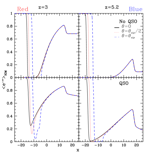
Figure 2: The transmitivity of a dynamic, infalling IGM surrounding a dark matter halo with total mass $M_{\rm tot}=5.2\times 10^{11}M_{\odot}$ at $z=3$ (Left Panels) and $z=5.2$ (Right Panels). The horizontal axis shows the frequency offset from the line center, in units of the Doppler width. The upper/lower panels show the transmission in the absence/presence of a central ionizing source in the halo with $L_{\rm ion}=5\times 10^{44}$ ergs s^-1, respectively. The solid–curve is the transmission from the center of our object, and is similar to the results found by Barkana & Loeb (2004). The dotted and dashed curves show the transmission at an angular impact parameter that corresponds to $0.5\theta_{\rm vir}$ and $1.0\theta_{\rm vir}$, respectively ($\theta_{\rm vir}$ is the angular size of the virial radius of the dark matter halo). The figure shows the IGM transmission reaches a minimum redward of the true line center for all models. Furthermore, the IGM transmission is a function of impact parameter especially on the red side of the Ly$\alpha$ line ($-10\;\hbox to0.0pt{\lower 2.5pt\hbox{$\sim$}\hss}\raise 1.5pt\hbox{$<$}\;x\;\hbox to0.0pt{\lower 2.5pt\hbox{$\sim$}\hss}\raise 1.5pt\hbox{$<$}\;0$), which may be important for a diffuse background source.

$$\tau_{x}(\theta)=\sigma_{0}\int_{r_{\rm vir}}^{\infty}dr\frac{r\hskip 2.84526ptn_{\rm IGM}(r)\hskip 2.84526ptx_{\rm H}(r)}{\sqrt{r^{2}-y^{2}}}\phi\Big{(}x-\frac{v_{\rm IGM}(r)}{v_{\rm th}}\big{[}1-\frac{y^{2}}{r^{2}}\big{]}^{1/2}\Big{)},$$ (2)

where $y\equiv\theta\times[r_{\rm vir}/\theta_{\rm vir}]$, and the integral over the line of sight $s$ has been converted to an integral over the radial coordinate $r$ measuring the distance from the center of the halo to points along the line of sight.

The final step in the calculation is to obtain the neutral fraction $x_{\rm HI}(r)$. As mentioned above, the mean transmission $\langle\exp{(-\tau)}\rangle$ is known observationally. Here the brackets denote averaging over the probability distribution of overdensities, arising from small-scale density fluctuations in the IGM. The averaging is over a spatial scale corresponding to the spectral resolution. We make the simple Ansatz that $\langle\exp{(-\tau)}\rangle$ equals $\exp{(-\tau_{0})}$, where $\tau_{0}$ is the transmittivity at the mean density and $x=0$,

$$\tau_{0}=\frac{\langle n_{\rm IGM}\rangle x_{\rm HI,0}v_{\rm th}\sigma_{0}}{H(z)},$$ (3)

where in the last step we used $ds=v_{\rm th}dx/H(z)$ (see Appendix A of paper I). From this Ansatz, we compute $x_{\rm HI,0}$, the neutral fraction at the mean density, and, assuming photoionization equilibrium, we compute the background flux $J_{\rm bg}$. For gas at overdensity $\delta\neq 0$, the neutral fraction then simply scales as $x_{\rm HI}(\delta)\propto(1+\delta)J_{\rm bg}^{-1}$. In the absence of a quasar, $J_{\rm bg}$ is constant, and in the presence of a quasar, we add the quasar’s flux, which scales as $J_{\rm Q}\propto r^{-2}$. For a realistic density probability distribution function (PDF), the transmission at the mean density can differ appreciably from $\langle\exp{(-\tau)}\rangle$. However, our simple treatment, by construction, will give the correct mean transmittivity, and effectively assumes only that the gas clumping factor $C=\langle\rho^{2}\rangle/\langle\rho\rangle^{2}$ due to small–scale inhomogeneities is independent of the overdensity $\delta$ on larger scales (corresponding to a spectral resolution element). More elaborate treatments would incorporate a model for the small–scale gas clumping. For example, Barkana & Loeb (2004) model the density PDF based on simulations. We find that our crude treatment yields comparable results for the transmission curves they obtained in their Figure 3 (especially when considering that their transmission will be reduced further near the line center in the absence of a quasar).

The IGM transmission we obtain is presented in Figure 2 in four different cases. The transmittivity is shown as a function of frequency $x$ for three different impact parameters, $\theta=0$ (solid–black curves), $\theta=0.5\theta_{\rm vir}$ (red–dotted curves) and $\theta=1.0\theta_{\rm vir}$ (blue–dashed curves). The upper panels show the transmission in the absence of any ionizing sources (apart from the uniform background), while the models shown in the lower panels include a source with a total ionizing luminosity of $5\times 10^{44}$ ergs s^-1. We assumed a quasar–like power–law spectrum for the source of the form $\propto\nu^{-1.7}$. Barkana & Loeb (2004) performed similar calculations for the IGM transmission. The three main differences in the work presented in this paper are (i) our simpler treatment of the small–scale gas clumping, (ii) the possibility that no bright ionizing quasar is present, and (iii) our spherically symmetric objects are spatially extended, and the IGM transmission depends on the impact parameter. The following can be inferred from Figure 2:

• The IGM is most opaque at frequencies around the line center. Depending on the exact model, the IGM’s opacity is at its maximum slightly redward of the true line center. The reduced IGM transmission extends to frequencies corresponding to $\sim v_{\rm circ}$, as already concluded by Barkana & Loeb (2003, 2004);

• In the absence of an ionizing quasar, the transmission is reduced to $\sim 0$ for a significant range of frequencies (whereas the transmission never drops to 0 in Barkana & Loeb, 2004, due to the presence of a bright quasar in their models). This range depends on the redshift, with attenuation decreasing at lower $z$, as shown by the difference between the left and right panels. In the presence of the ionizing source, the attenuation is significantly reduced, as shown by comparing the upper and lower panels.

• The IGM transmission is a function of impact parameter. The frequency range with strong attenuation diminishes at larger impact parameters, due to the smaller projected peculiar velocity of the IGM.

2.4 Impact of a Dynamic IGM on the Results from Paper I.

First, we show how the IGM modifies the spectrum emerging from the fiducial model 1 from paper I. The left panel of Figure 3 shows the flux (in arbitrary units) as a function of frequency, $x$, for the intrinsic (blue–dotted line) and observable (black–solid line) cases. Since model 1. concerns the collapse of a neutral hydrogen cloud (i.e. no embedded ionizing source is present), the IGM transmittivity from Figure 2 for the ‘no qso’ case (upper panels) is taken. For this plot, the redshift of the Ly$\alpha$ source was assumed to be $z=3$. In the right panel, the flux is shown as a function of observable wavelength.

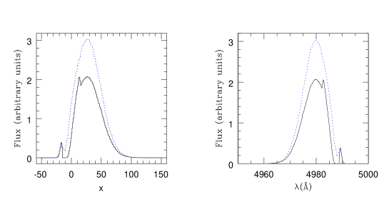
Figure 3: The impact of the IGM on the spectrum from our fiducial model 1. The left panel shows the intrinsic (blue–dotted line) and observable (black–solid line) spectra. The IGM transmittivity from the upper left panel of Fig. 2 is taken. In the right panel, the spectrum is shown as a function of observable wavelength. The figure shows that the IGM suppresses the blue peak and enhances the prominence of the dip between the red and blue peak.

The main effects of the IGM here are to suppress the blue peak and to enhance the prominence of the dip between the blue and red peak. We note that the dip remains at the same location. For the spectra emerging from the central models, the photons emerge with a larger average blue shift (with practically no photons redward of the line center), and for these models the main effect of the IGM is to suppress the total Ly$\alpha$ flux.

Second, we discuss how the IGM modifies the surface brightness profiles. In the absence of a quasar (or any other ionizing source), the IGM becomes more transparent with $\theta$ for photons in the red peak. The result of this is that the surface brightness profiles of the reddest photons ($x\;\hbox to0.0pt{\lower 2.5pt\hbox{$\sim$}\hss}\raise 1.5pt\hbox{$<$}\;-10$) appears flatter than those calculated in paper I. This would strengthen the result that for neutral collapsing protogalaxies (i.e. in the absence of an ionizing source), the reddest Ly$\alpha\hskip 2.84526pt$photons appear less centrally concentrated than the bluest Ly$\alpha\hskip 2.84526pt$photons (see Figure 10 in paper I).

In the presence of a quasar (or any other ionizing source), the IGM also flattens the surface brightness profile of the reddest photons ($x\;\hbox to0.0pt{\lower 2.5pt\hbox{$\sim$}\hss}\raise 1.5pt\hbox{$<$}\;-10$). However, the transmission of the IGM can decrease with increasing $\theta$ for a range of frequencies, $0\;\hbox to0.0pt{\lower 2.5pt\hbox{$\sim$}\hss}\raise 1.5pt\hbox{$<$}\;x\;\hbox to0.0pt{\lower 2.5pt\hbox{$\sim$}\hss}\raise 1.5pt\hbox{$<$}\;-10$, e.g. at $x\approx-10$ in the lower panels of Fig. 2. This is because at larger impact parameters, there can be a large effective column of absorbing material at projected velocity smaller than the maximum IGM infall speed. For photons in this frequency range, the IGM steepens the surface brightness profiles.

The exact dependence of the IGM transmission on frequency and impact parameter in the presence (and absence) of an ionizing source depends strongly on the exact assumed density and velocity field of the gas in the IGM. Furthermore, the IGM is unlikely to collapse in a spherically symmetric fashion. This introduces uncertainties to the angular dependence of the IGM transmission whose modeling is beyond the scope of this paper. Despite these uncertainies, the main impact of the IGM on the results obtained in paper I is clear:

• The result that a steepening of the surface brightness profile towards bluer wavelengths within the Ly$\alpha$ line is a useful diagnostic for gas infall, is not affected by the IGM.

• The result that infall and outflow models can produce nearly identical spectra, may be affected by the IGM. The reason is that the IGM transmission is asymmetric around $x=0$. Below (§ 3.1.2), we show that scattering in the IGM may cause emission lines that have identical profiles, but differ only by a small ($\sim$ several Doppler widths) frequency shift (caused by either inflow or outflow), may have somewhat different observed values of $[B]/[R]$ (defined in paper I as the ratio of the number of photons in the blue and red peak).

• All other results relating to (i) the net blueshift of the blue peak, (ii) FWHM of the blue peak, (iii) the location of the red peak (if any), (iv) the ratio $[B]/[R]$ and its dependence on mass, gas infall velocity and redshift are not affected significantly by the IGM.

With this knowledge at hand, and keeping in mind that a dynamic IGM may produce an absorption feature slightly redward of the true Ly$\alpha$ line center, we interprete several observations of known Ly$\alpha$ emitters below.

3 Comparison with Observed Lyman $\alpha$ Sources

It will be useful to explicitly recall a result from paper I, in which we found the total observable Ly$\alpha$ cooling radiation flux from an object of mass $M_{\rm tot}$, collapsing at redshift $z_{\rm vir}$, to be approximately

$$\frac{f_{{\rm Ly}\alpha}}{10^{-18}}\approx 2\hskip 2.84526ptf_{\alpha}\hskip 2.84526pt\Big{(}\frac{M_{\rm tot}}{10^{11}M_{\odot}}\Big{)}^{\frac{5}{3}}\Big{(}\frac{v_{\rm amp}}{v_{\rm circ}}\Big{)}\Big{(}\frac{2-\alpha}{1.75}\Big{)}^{1.2}\times$$

$$\left\{\begin{array}[]{ll}\ \times(\frac{5}{1+z_{\rm vir}})^{1.75}&z\leq 4.0\\ \\ \ \times(\frac{5}{1+z_{\rm vir}})^{8.3}&z>4.0\end{array}\right.\hskip 2.84526pt\frac{{\rm ergs}}{{\rm sec}\hskip 2.84526pt{\rm cm}^{2}},$$ (7)

where $f_{\alpha}$ is the fraction of binding energy going into the Ly$\alpha$ line. Other model assumptions included: 1) The gas density profile was assumed to trace that of the dark matter at large radii, but with a finite core. The emissivity profile was calculated self–consistently by computing the rate of change in the gravitational binding energy at each radius; 2) The infall velocity of the gas was taken to be of the form $v_{\rm bulk}(r)=-v_{\rm amp}(r/r_{\rm vir})^{\alpha}$. The $\alpha$ dependence of $f_{{\rm Ly}\alpha}$ is a fit that is valid for the range $\alpha\in[-0.5,1]$ (see paper I for more details on our models).

We caution that the strong break in the slope of the redshift dependence of the flux (eq. 7) at $z=4$ should not be taken literally. In reality, the variation of the this slope with redshift should be smoother. The main point of eq. (7) however, is that because the IGM becomes increasingly opaque towards higher redshifts at $z\gtrsim 4$, cooling radiation of a fixed luminosity is more difficult to detect at $z\gtrsim 4$ than at $z\;\hbox to0.0pt{\lower 2.5pt\hbox{$\sim$}\hss}\raise 1.5pt\hbox{$<$}\;4$. Quantitatively, the total detectable Ly$\alpha$ cooling flux does not scale with $d_{L}^{-2}$ (which can be approximated as $\propto(1+z)^{-2.75}$), but as $\propto<e^{-\tau}>d_{L}^{-2}$ (which can be approximated as $\propto(1+z)^{-11}$) for $z\geq 4.0$.

In paper I, we studied a range of models with different masses, redshifts, and emissivity, density, and velocity profiles. Table 2 summarizes the parameters of two of paper I’s fiducial models and two models used in § 3.2. For each model the table contains the total mass, redshift, and circular velocity of the host halo, as well as the parameters describing the infall velocity field. For each model, all gas continously emits all its gravitational binding energy as Ly$\alpha$ as it navigates down the dark matter potential well (in the terminology of paper I, these are ’extended’ models with $f_{\alpha}=1.0$).

Table 2: Model Parameters

Model #	$M_{\rm tot}$	$z_{\rm vir}$	$v_{\rm circ}$	$v_{\rm amp}$	$\alpha$	$f_{\alpha}$
(Ext.)	$10^{11}M_{\odot}$		km s-1	$v_{\rm circ}$
1	5.2	3.0	181	1.0	1.0	1.0
2	5.2	3.0	181	1.0	-0.5	1.0
M1	15	3.0	257	1.0	1.0	1.0
M2	15	3.0	257	1.0	-0.5	1.0

3.1 Comparison with Steidel et al’s LABs.

We start our comparison with the data presented in Steidel et al. (2000), who found two large, diffuse, and relatively bright Ly$\alpha$ emitters (‘Ly$\alpha$ blobs’ or ’LABs’) in a deep narrow band search of a field known to contain a significant overdensity of Lyman Break galaxies. The total observed flux is $\sim 10^{-15}$ ergs s^-1 cm^-2 for each blob, and both have a physical size exceeding $140$ kpc. The excitation or ionization mechanism for either blob is poorly understood. One blob, referred to as ‘LAB1’, has a bright sub–mm source as a counterpart (with some uncertainty in the identification, given the 15” half power beamwidth; Chapman et al., 2004). The physical interpretation is that a dust enshrouded AGN, which is undetected at other frequencies, is buried within the Ly$\alpha$ halo. It has been speculated that a jet–like structure that is well outside of our line of sight induces star formation, which, combined with the ionizing radiation from the AGN, photo-ionizes the surrounding hydrogen cloud (Chapman et al., 2004). The other blob, ‘LAB2’, has no sub-mm bright counterpart, but Basu-Zych & Scharf (2004) have found an associated hard X-ray source in Chandra archival data, with a total luminosity comparable to that of the Ly$\alpha$ ($L\sim 10^{44}$ ergs s^-1). Basu-Zych & Scharf (2004) have speculated that both LAB1 and LAB2 may have an embedded AGN, which goes through periodic episodes of activity. An old population of relativistic electrons, originating near the supermassive black hole that powers the AGN, can upscatter CMB photons into the X-ray band, which may then illuminate the hydrogen gas and explain at least part of the Ly$\alpha$ flux in these blobs. This scenario is based on interpretations of recent findings of extended X-ray sources at redshifts as high as $z=3.8$ (e.g. Scharf et al., 2003).

The possibility that cooling radiation contributes significantly to Ly$\alpha$ flux of the LABs remains. First, we notice that to produce a flux of $10^{-15}$ ergs s^-1 cm^-2 from cooling radiation alone, requires $v_{\rm circ}\sim 300$ km s^-1 or $M_{\rm tot}\sim 2-3\times 10^{12}f_{\alpha}^{-3/5}\hskip 2.84526ptM_{\odot}$. The virial radius of an object of this mass is $\sim 100f_{\alpha}^{-1/5}$ kpc, corresponding to $\sim 13$ $f_{\alpha}^{-1/5}$ ”, in good agreement with the observed size of the blobs. Given that the image can be observed over a large region on the sky suggests that the surface brightness profile is not declining rapidly with radius, which argue against our “central” model. More quantitatively, Figure 9. of paper I shows that $\partial\ln F$ / $\partial\ln\theta$ $\;\hbox to0.0pt{\lower 2.5pt\hbox{$\sim$}\hss}\raise 1.5pt\hbox{$<$}\;-2$ and $\;\hbox to0.0pt{\lower 2.5pt\hbox{$\sim$}\hss}\raise 1.5pt\hbox{$>$}\;-1$ for the central and extended models, respectively for $M=4\times 10^{12}{\rm M}_{\odot}$. The plots in Steidel et al. (2000) lack contour levels, but especially the surface brightness of fainter emission does not appear to rapidly decrease with radius.

For extended cooling radiation, the Ly$\alpha$ spectrum should be double peaked (provided the red peak is not swallowed by the blue, but for $v_{\rm amp}\sim v_{\rm circ}\sim 300$ km s^-1, this is not expected according to our findings in paper I). Steidel et al. (2000) present spectra taken along slits across both blobs. More recently, however, Bower et al. (2004) and Wilman et al. (2005) have used the SAURON Integral Field Spectrograph to observe Steidel et al. (2000)’s LAB1 and LAB2, respectively. Since these spectra cover the entire two–dimensional region of Ly$\alpha$ emission, we use these more recent spectra for comparisons to our models.

3.1.1 Comparison with Spectra of LAB1

The spectra presented by Bower et al. (2004) have a complex structure. If LAB1 is emitting cooling radiation, surrounded by an extremely optically thick ($\tau\;\hbox to0.0pt{\lower 2.5pt\hbox{$\sim$}\hss}\raise 1.5pt\hbox{$>$}\;10^{6}$) collapsing hydrogen cloud, the Ly$\alpha$ radiation is expected to emerge with a net blue shift. It is not possible to tell from Bower et al. (2004)’s data whether this is the case, since, in the absence of other lines, the systemic redshift of the LAB is not known. There is no evidence for a fainter redder peak. In Steidel et al. (2000)’s original data, there is evidence that the main bluer peak is accompanied by a fainter redder peak, with $[B]/[R]\gg 1$. Unfortunately, it is not possible to calculate the exact value of $[B]/[R]$ from Steidel et al. (2000)’s paper, since the contour levels of their spectra are not shown. In our fiducial model, but with the mass of the halo increased to $M_{\rm tot}=3\times 10^{12}{\rm M_{\odot}}$, as required by the angular size and total flux from LAB1, we expect $[B]/[R]\sim 100$ after including the effect of the IGM opacity (see Figure 8 in paper I for how the [B]/[R] ratio scales with various parameters). A secure detection of a double–peaked, asymmetric profile, with a stronger blue peak, $[B]/[R]\gg 1$, would be strong evidence for an optically thick, collapsing gas cloud. Bower et al. (2004) note that the line width appears to increase with radius, a feature that does not arise in models of neutral collapsing gas clouds presented in paper I. However, it does arise in models in which an ionized source is embedded within the gas cloud (see Fig. 13 of paper I). Indeed, the presence of a sub–mm source suggests that an ionizing source resides within LAB1. The ionizing source can not, however, fully ionize the gas (Fig. 13 in paper I), without violating $[B]/[R]\gg 1$ as observed by Steidel et al. (2000).

The origin of the Ly$\alpha\hskip 2.84526pt$emission in our model is then attributed to fluorescent radiation emitted in an HII region created by the central ionizing source. This HII region is surrounded by a neutral collapsing hydrogen envelope. Cooling radiation, generated over a spatially extended region within the neutral hydrogen envelope, may provide an additional contribution to the Ly$\alpha\hskip 2.84526pt$luminosity. Evidence for this scenario would be (i) a flat surface brightness profile, (ii) the strong asymmetry of the double–peaked profile ($[B]/[R]\gg 1$) and (iii) the increase of the FWHM of the line with radius. This interpretation is consistent with that given by Bower et al. (2004).

We note that Ohyama et al. (2003) have also obtained deep spectroscopy in a slit across LAB1, and showed that the spectrum of the brightest knot in particular, is more complex than can be explained with our models. The spectrum of the central knot can be be fitted with three Gaussians, each separated by $\sim 2000$ km s^-1. The other regions are consistent with our model above.

3.1.2 Comparison with Spectra of LAB2

LAB2 has a complicated morphology, with six distinct sub–blobs of resolved Ly$\alpha$ emission. The spectra of the sub–blobs all exhibit a double–peaked frequency structure. Wilman et al. (2005) show that the spectra can be explained with a very simple model. The emission line is assumed to be a Gaussian with a FWHM of $\sim 1000$ km s^-1, with its peak frequency varying by $\sim 290$ km s^-1 over the entire LAB. A foreground slab of neutral gas with $N_{HI}\sim 10^{19}$ cm^-2 leaves an absorption feature which falls at the same wavelength in all six spectra. Wilman et al. (2005) attribute this absorption feature to a foreground shell of neutral hydrogen gas, swept up by a galaxy–sized outflow. Indeed, in four out of six sub–blobs (except for B and F), the absorption line lies blueward of the peak of their Gaussian emission line. We show below, however, that these data can also be explained with an equally simple in–fall model.

In our model, we take the same intrinsic emission profile of the Ly$\alpha$ emission as in Wilman et al. (2005), and likewise, we allow ourselves the freedom to shift the peak frequency of the intrinsic emission to the blue by up to $\sim 300$ km s^-1 (see the shift assumed in each panel). We process this emission line through the model of the dynamic IGM as discussed in § 2. We calculated the IGM transmission curves expected for a source with $M_{\rm tot}=10^{12}M_{\odot}$ and added an ionizing source with $L_{\rm ion}=2\times 10^{44}$ ergs s^-1 to increase the transmission near the line center (Note that we assumed $\theta=0$ in eq. 2 for all panels, as discussed in § 2). The results are shown in Figure 4, which can be compared directly to Figure 3 in Wilman et al. (2005). Our model provides an equally good fit to the data. Further improvement of the fits is possible, if we allow ourselves the freedom to vary the IGM model (and the exact shape of the emission line) from location to location on the sky, rather than imposing a single IGM infall model as we have done.

To understand why our model provides a good fit is through the IGM transmission curve shown in lower left panel of Figure 2. Panel D in Figure 4 is obtained by multiplying a Gaussian emission line that is centered on the line center ($x=0$), by this IGM transmission. Shifting the Gaussian back and forth in frequency and multiplying these emission lines by this transmission curve yields the results shown in Figure 4. Each panel contains the required velocity shift in its top right corner. A negative velocity corresponds to a blue shift of the line.

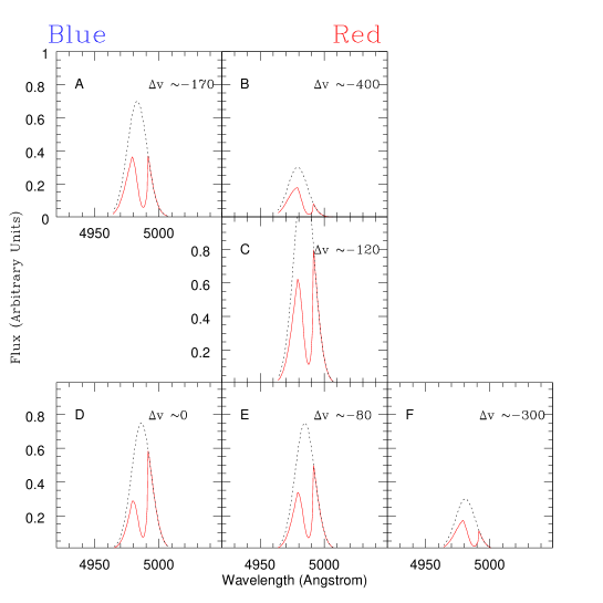
Figure 4: A reproduction of the observed Ly$\alpha$ spectra of Steidel et al’s LAB2 by Wilman et al. (2005). The spectra in the different panels are displayed in the same way as originally in Wilman et al. (2005), who succesfully reproduced their observations with a foreground shell of neutral hydrogen gas, swept up by a galaxy–sized outflow. This figure demonstrates that our infall model reproduces the observed spectra of LAB2 equally well. Our model assumes simple infall for the IGM, as outlined in § 2. The red-solid lines are the spectra after scattering by the IGM. The solid-black lines are the intrinsic spectra. The spectra in panels B and F, with enhanced blue peaks, are consistent with cooling radiation that is propagating outwards through the collapsing, neutral hydrogen gas.

First we point out that all panels, except for panel D, require an intrinsic blue shift of the emission line. This requires the gas within the virial radius to be collapsing. Second, the spectra in panels B and F, which are the two farthest out–lying sub–blobs in the two–dimensional image of LAB2, have enhanced blue peaks, requiring a significant blueshift in the intrinsic emission, by $\sim 3-400$ km s^-1. Within our model, this blue–shift would naturally arise if the gas far out at the locations of sub–blobs B and F is collapsing and optically thick ($\tau_{\alpha}\gtrsim 10^{4}$) to Ly$\alpha$ photons. The smaller intrinsic required blueshift in panels A, C and E can be accounted for if the Ly$\alpha$ photons were propagating outwards through gas that is photoionized by an embedded ionizing source (see Figure 11 in paper I). Wilman et al. (2005) show in their Figure 2 that regions B and F are also significantly fainter than the other sub–blobs. This would again be expected the Ly$\alpha\hskip 2.84526pt$radiation emerging from these regions were attributed to cooling radiation (as opposed to photoionization for the other sub–blobs, which reside closer to any embedded ionizing source). Our physical picture associated with the collapse is that the gas is collapsing as a whole onto their mutual center of mass. Panels B & F show Ly$\alpha$ cooling radiation, generated over a spatially extended region. The Ly$\alpha$ emission from the blobs in the other panels consists of processed ionizing radiation from embedded ionizing sources. The IGM surrounding LAB2 is dragged along in the overall cloud collapse.

Based on the data on the two Ly$\alpha$ blobs presented in Steidel et al. (2000), we conclude that the spectrum and surface brightness distribution of LAB1 are consistent with a model in which gas is collapsing in a DM halo with $M_{\rm tot}=$ a few $\times 10^{12}M_{\odot}$ while emitting fluorescent Ly$\alpha$ radiation in response to photoionization by (an) embedded ionizing source(s) (except the brightest knot, which is likely powered by an outflow Ohyama et al., 2003). We found that the spectra of LAB2 can be explained if the intrinsic Ly$\alpha$ emission profile is a single Gaussian, blue–shifted by up to several hundred km/s due the collapse of optically thick gas within a massive halo, and subsequent resonant scattering on larger scales within a perturbed IGM.

3.2 Comparison with Matsuda et al.’s LABs

More recently, Matsuda (2004) published a catalogue of an additional 33 LABs, discovered in a deep, narrow–band, wide field (31’ $\times$ 23’) search with Subaru, centered on the same field as studied by Steidel et al. (2000). One third of their blobs are not associated with bright UV sources, and thus provide good candidates for objects dominated by cooling radiation. Mori et al. (2004) have used ultra–high resolution simulations to model a forming galaxy undergoing multiple epochs of supernova explosions and found their models could reproduce the typical Ly$\alpha$ luminosities observed from these LABs. Their models are particularly successful in reproducing the ’bubbly’ appearance of several LABs. Matsuda (2004) suggest that five specific Ly$\alpha$ blobs may be cooling objects, based on the diffuse appearance of the images. A diffuse appearance, may not be a necessary requirement for cooling radiation. The physical picture associated with extended cooling is that clumps of cold gas are flowing inwards, while emitting Ly$\alpha$ in response to various sources of heating (i.e. gravitational shock heating and possibly photoionization heating by the thermal emission from the hot, ambient gas). Therefore, some clumpiness in the surface brightness distribution may be expected. If we drop the requirement that the Ly$\alpha$ image is diffuse, then the number of candidates for cooling objects is increased to $12$.

The detected fluxes for the majority of the LABs lie in the range $7\times 10^{-17}-2\times 10^{-16}$ ergs s^-1 cm^-2, which correspond to cooling radiation from objects in the mass range $M_{\rm tot}\sim 1-2$ $\times 10^{12}f_{\alpha}^{-3/5}M_{\odot}$, for extended models with $(v_{\rm amp},\alpha)$ $=(v_{\rm circ},1)$ (see eq. 7). The corresponding range in virial radii is $\sim 80-100f_{\alpha}^{-1/5}$ kpc, which translates to an angle on the sky of $\sim 10-12f_{\alpha}^{-1/5}$”. Converting this to an area yields values which exceed the observed Ly$\alpha$ isophotal area by a factor of $\sim 10$. This is not surprising since the calculated surface brightness distribution may drop below the detection threshold in the outer parts. This is illustrated in Figure 5, in which we plot the surface brightness profile for model M1 as the red–dotted line. This is equivalent to our fiducial model, but with $M_{\rm tot}$ increased to $1.5\times 10^{12}M_{\odot}$. The total flux on earth for this model is predicted to be $1.6\times 10^{-16}$ ergs s^-1 cm^-2.

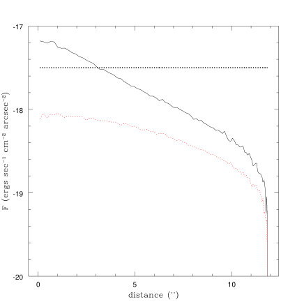
Figure 5: The figure shows the surface brightness profile of a model that has the observed gross properties of the majority of the blobs found by Matsuda (2004) (black solid line, see text). If this model is correct, then deeper observations will reveal these blobs to be spatially more extended. The red dotted line represents the same model with $\alpha$ changed from $-0.5$ to $1.0$. This object would escape detection since its surface brightness is everywhere below Matsuda (2004)’s detection limit, indicated by the thick–dotted horizontal line.

From Figure 5, however, it can be seen that this radiation is too diffuse to be detected. The total flux is spread over an area of $\sim 300$ arcsec², which brings the average surface brightness below the detection threshold of $3\times 10^{-18}$ ergs s^-1 cm ^-2 arcsec^-2. The flux is more centrally concentrated for models with lower $\alpha$ (see paper I). Plotted as the black–solid line, is the surface brightness profile of model M2, which is identical to model M1, except with $\alpha=-0.5$. For this model, the flux from the inner 3” exceeds the detection limit. The total flux from this detectable region is $1.5\times 10^{-16}$ ergs s^-1 cm^-2, which is spread over an area of $\sim 30$ arcsec². This angular extent is consistent with the observed area of the majority of Ly$\alpha$ blobs, $20-40$ arcsec². The average surface brightness of the detectable region of model M2 is $\sim 5.2\times 10^{-18}$ ergs s^-1 cm ^-2 arcsec^-2, which corresponds to $m_{AB}\sim 27.1$ mag arcsec^-2. Matsuda (2004) focussed on imaging and did not present spectra in their paper, so further comparison is at this stage not possible. If this model is correct, then deeper observations will reveal these sources to be spatially more extended. We showed in Figure 10 of paper I that for extended models with $\alpha=-0.5$, the bluest 15$\%$ of the Ly$\alpha$ photons would appear more centrally concentrated than the reddest $15\%$. Comparing Figure 10 from paper I and Figure 5 suggests that the surface brightness of the reddest $15\%$ of the photons may have been below the detection limit, implying that deeper observations may reveal the red peak in the spectrum (if it is not already in the data).

3.3 Spectroscopic Detections

Our comparisons have so far focused on extended LABs, which are a rarity among the known Ly$\alpha$ emitters. As mentioned in § 1, narrow band searches on Kitt Peak (LALA, e.g. Rhoads et al., 2000; Rhoads & Malhotra, 2001; Rhoads et al., 2004), on Keck (e.g. Hu et al., 1998) and on Subaru (e.g. Kodaira, 2003; Hu et al., 2004; Ouchi, 2005), have been very successful in finding galaxies at redshifts $z\geq 4.5$. The narrow band surveys, combined with deep broad band images, provide candidates based on selection criteria involving the colors, equivalent widths, and flux thresholds. These candidates need spectroscopic confirmation, using large telescopes such as the Very Large Telescope (VLT) and Keck. Roughly $30\%$ of the candidates are confirmed to be genuine high redshift Ly$\alpha$ emitters (e.g. Hu et al., 2004). Contrary to the lower redshift LABs, these Ly$\alpha$ emitters thus all have observed spectra. The known Ly$\alpha$ emitters typically have total fluxes in the range $5\times 10^{-18}-5\times 10^{-17}$ ergs s^-1 cm^-2, which is fainter by at least an order of magnitude than the LABs discussed above.

If some of these Ly$\alpha$ emitters are cooling objects, then deeper observations will reveal fainter, more diffuse emission associated with them (unless the emission is strongly centrally concentrated, in which case the surface brightness profiles drops rapidly, see Fig. 11 of paper I). To produce a detectable flux of $10^{-17}$ ergs s^-1 cm^-2 from a $z=5.7$ source requires $M_{\rm tot}\sim 10^{12}M_{\odot}$ (eq. 7). A dark matter halo of this mass that collapses at $z=5.7$ is associated with a $\sim 3\sigma$ fluctuation in the primordial density field. According to the Press-Schechter mass function, the number density of halos with $M>10^{12}M_{\odot}$, is $1.3\times 10^{-5}$ Mpc^-3 at $z=5.7$, which is factor of $\sim 40$ lower than the implied number density of Ly$\alpha\hskip 2.84526pt$emitters at this redshift (e.g. Ouchi, 2005). Additionally, the typical observed flux from a Ly$\alpha$ emitter of $10^{-17}$ ergs s^-1 cm^-2 comes from a small region, $\sim 1$ arcsec². This implies that either all cooling radiation from this $M_{\rm tot}=10^{12}M_{\odot}$ object emerges from this small area, which requires the surface brightness profile to be very steep, and thus favor the central models (§ 1). Alternatively, we could be detecting the brightest central region a spatially extended Ly$\alpha$ halo (as in Fig. 5). This, however, would require an even more massive, and therefore even rarer, halo to produce the measured Ly$\alpha$ flux levels. The above suggests that the majority of the known high redshift Ly$\alpha$ emitters are not powered by cooling radiation alone. Indeed, the continuum detection of many high redshift Ly$\alpha$ emitters, which show that the equivalent width of the Ly$\alpha$ line is consistent with ionization by young stars forming with a usual IMF.

An object of particular interest to us is described by Bunker et al. (2003b), who discovered a $z=5.78$ galaxy with a total Ly$\alpha$ flux of $2\times 10^{-17}$ ergs s^-1 cm^-2 in the Chandra Deep Field-South. Using the DEIMOS spectrograph on Keck, they obtained a spectrum, which looks remarkably like the spectrum for a ’extended’ model: a small red peak is separated from a more pronounced bluer peak by $\sim 400$ km s^-1. If powered by cooling radiation, a total flux of $2\times 10^{-17}$ ergs s^-1 cm^-2 would require gas cooling in a halo with a mass of $M\sim 10^{12}M_{\odot}$. If the gas in this object were continuously cooling, this would produce the maximum of the red peak to lie $>300$ km s^-1 from the line center. The problem with this interpretation however, is that the Ly$\alpha$ emission is extremely compact, with an angular size less than $\sim 0.1^{\prime\prime}$. Since the emission is detected at the $20-\sigma$ level, this implies that the surface brightness falls of by a factor of $\;\hbox to0.0pt{\lower 2.5pt\hbox{$\sim$}\hss}\raise 1.5pt\hbox{$>$}\;20$ over $\sim 0.1^{\prime\prime}$. Because extended cooling models have rather flat surface brightness distributions (with $\partial\ln F$ / $\partial\ln\theta$ $\sim-1$ to $-0.5$, see paper I), they are not consistent with the observed compactness of the emission. A similar conclusion applies to the faint, strongly gravitationally lensed Ly$\alpha$ emitter discovered recently behind a galaxy cluster (Ellis et al., 2001), which remains a point–source despite the large increase in the effective spatial resolution afforded by the presence of strong lensing.

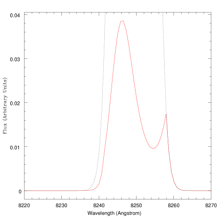
Figure 6: This figure shows a the spectrum of a model that is consistent with recent observations by of a $z=5.78$ Ly$\alpha$ emitter in the Chandra Deep Field–South by Bunker et al. (2003b). An infalling IGM, as outlined in § 2, can modify the intrinsic Gaussian emission line (indicated by the black–dotted line) to have a dip in the observable spectrum (indicated by the red–solid line) on the red side of the line.

An alternative interpretation of this spectrum combined with the compactness of the emission is that the Ly$\alpha$ emission is due to stars in an already formed galaxy, as Bunker et al. (2003b) argue, that fully photoionizes the gas in the galaxy. The emission line is therefore centered on the true line center and its FWHM set by the gas’ velocity dispersion. If we process this Ly$\alpha$ through an infalling IGM, as described in § 2, we find we can reproduce the gross features of the observed spectrum, as shown in Figure 6 by the solid–red line. The intrinsic line profile is given by the black–dotted line. In this model, the IGM scatters $\sim 95\%$ of the Ly$\alpha$ photons out of the line of sight. It is generally assumed that the IGM only allows photons from high–z Ly$\alpha$ emitters to be detected on the red half of the Ly$\alpha$ emission line, implying $\sim 50\%$ is scattered out of our line of sight. If our model is correct then the intrinsic luminosity may of this Ly$\alpha$ emitter may have been underestimated by a factor of $\sim 10$. The intrinsic Ly$\alpha$ equivalent width would then be increased from 20 to $\sim 200$ Å. This could have important consequences: if the intrinsic Ly$\alpha$ luminosity has been systematically underestimated for high–z Ly$\alpha$ emitters, then the escape fraction of Ly$\alpha$ photons would have to be unusually high (for a constant star formation rate). This may put interesting limits on the dust abundance and/or distribution in these galaxies. Alternatively, it could imply that estimates of the total intrinsic Ly$\alpha$ luminosity must be revised, requiring a $\sim 10$ times larger star–formation rate. The latter would enhance the implied contribution of high redshift Ly$\alpha$ emitters to the ionizing background. Either way, these issues deserve more attention and will be addressed in more detail elsewhere (Dijkstra et al., 2006). We emphasize that the only requirements for these issues to be relevant for a Ly$\alpha$ emitter are that i) its surrounding IGM is collapsing, and ii) its intrinsic emission line is not redshifted significantly ($v_{\rm shift}\;\hbox to0.0pt{\lower 2.5pt\hbox{$\sim$}\hss}\raise 1.5pt\hbox{$>$}\;v_{\rm circ}$, but note this can easily be achieved in outflows).

4 Discussion

As argued above, observational evidence exists for gas infall around both pointlike (§ 3.3) and extended (§ 3.1.2) Ly$\alpha$ emitters. Below (§ 4.1) we compare our model for Steidel et al. (2000)’s LAB2 with a recently proposed outflow model by Wilman et al. (2005). We discuss why two such different mechanisms can reproduce the observed spectra well. We argue in § 4.2 that the notion that infall models may produce similar Ly$\alpha$ spectral features as outflow models may be more generic and discuss its cosmological implications. In § 4.3 we discuss how additional imaging in H$\alpha$ may help to resolve this issue.

4.1 Infall vs. Outflow in Steidel et al’s LAB2

It may come as a surprise that two completely different mechanisms (infall vs. outflow) may reproduce the observed spectra of Steidel et al. (2000)’s LAB2. To produce a spectrum with $[B]/[R]<1$ using a single absorbing shell of material, the shell must absorb on the blue side of the emission line, and must therefore be outflowing. As mentioned above, an infall model naturally produces $[B]/[R]<1$ (shown in Fig. 2). Note that the for the exact same intrinsic emission line and the same $[B]/[R]$ ratio, the dip in the spectra for the outflow and infall model lies blueward and redward of the true line center, respectively. This difference is in practice difficult to see, especially since the intrinsic emission line is unlikely to be Gaussian (see Fig. 3 and paper I, in which we calculated the exact shape of the emission line emerging from models of both neutral and photoionized collapsing gas clouds). We caution that the isotropically infalling IGM will not change the total flux toward Earth. However, the scattering ”IGM shell” is geometrically quite thick (up to $\sim 5$ virial radii ), so any photons scattered back into our line of sight will be spread over a large solid angle (and also spread in frequency). This ”super-fuzz” is too diffuse to modify the simple absorption dip due to scattering out of the line of sight.

An advantage of our explanation is that the intrinsic blue shift of the emission line, in all panels, is consistent with overall gas collapse. The amount of blueshift of each line is determined by the brightness of the photoionized source. Indeed, the brightest Ly$\alpha$ blobs have the smallest net blue shift.

A second advantage of the above explanation of the data is that it may require less fine tuning than the explanation by the swept–up shell, given by Wilman et al. (2005). The peak frequency of the absorption dip varies by less than $60$ km s^-1 among the six different sub–blobs covering LAB2. This small variation would arise naturally if the entire shell has virtually stalled and come to rest with respect to the galaxy’s systemic velocity. Because a superwind will spend most of its time close to the zero velocity stalling radius it is most likely observed at this position. However, for the shell to stall and preserve a similar column density over large length scales (a few $100$ kpc) and long times ($10^{8}$ yrs), requires the ambient pressure of the IGM not to exhibit pressure gradients on these scales. In our model, the IGM infall velocity is $\sim 300$ km s^-1 and may vary by $\sim 20\%$ over the entire blob and may be a less stringent requirement.

In either model, the difference between LAB1 and LAB2 remains a puzzle. If the shape of the observed spectrum in LAB2 is indeed due to IGM infall, then this IGM infall is also expected around LAB1. However, no evidence for this is seen in the spectra of in LAB1. In our infall model, this would require that the Ly$\alpha$ flux emerges across LAB1 with a larger intrinsic blueshift of $\sim 500$ km s^-1. As we showed in paper I, this can be easily reached when the gas in LAB1 is optically thick ($\tau_{\alpha}\;\hbox to0.0pt{\lower 2.5pt\hbox{$\sim$}\hss}\raise 1.5pt\hbox{$>$}\;10^{4}$) to the Ly$\alpha$ photons.

4.2 Infall vs. Outflow in all Ly$\alpha$ Emitters

Ample spectroscopic evidence exist for outflows of gas around Lyman Break Galaxies (LBGs, e.g. Adelberger et al., 2003, and references therein). It is not yet securely established to what level these superwinds surround the galaxy (i.e. what solid angle around the galaxy is swept up by the wind). The physical extent of the superwind is set by the star formation history of its host galaxy, and determines to what degree it can prevent gas from the IGM to continue to cool and collapse onto the galaxy. Understanding superwinds is clearly a requirement for understanding galaxy formation and evolution. Wilman et al. (2005) have argued that their recent observations demonstrate that superwinds occur on galactic scales around Steidel et al. (2000)’s LAB2. However, we showed in § 3.1 above that these observations are also consistent with an inflowing IGM.

One may argue that the number of LBGs with known outflows greatly outnumber the number of known inflows. However, this does not necessarily imply that galaxies with outflows are more common than those with significant gas infall. At high redshifts, $z\gtrsim 5$, candidates for galaxies containing a superwind are found based on their Ly$\alpha$ properties (see Taniguchi et al., 2003, for a review). As in the case of LAB2, some of the Ly$\alpha$ spectra of candidate superwind galaxies (e.g. Dawson et al., 2002) could in fact also be explained by infall of the IGM (Dijkstra et al, 2006b, in prep) onto the Ly$\alpha$ emitter. Additionally, for a given intrinsic Ly$\alpha$ luminosity, there is observational bias to detect an outflow. The intrinsically redshifted Ly$\alpha\hskip 2.84526pt$emission from outflows is easier to detect than the blueshifted Ly$\alpha$ from infall, because the latter will be subject to much more severe attenuation in the IGM. Furthermore, outflows can be more compact than large scale infall, increasing the surface brightness. These observational biases must be accounted for when calculating the fraction of Ly$\alpha$ emitters associated with outflows and infall. With ongoing and future Ly$\alpha$ surveys, the sample of high redshift Ly$\alpha$ emitters steadily grows, allowing a better determination of this number, and addressing various basic questions related to galaxy formation: (i) how common is Ly$\alpha$ cooling radiation among collapsing protogalaxies? (ii) how common is fluorescent Ly$\alpha$ emission due to embedded ionizing sources (such as a central quasar or young stars that formed during the collapse) among protogalaxies? iii) how common are superwinds in young galaxies at high redshifts?

4.3 H$\alpha$ Emission from Protogalaxies

Discussion of emission line radiation from protogalaxies have focused typically on Ly$\alpha$ radiation, but as argued by Oh (1999), the H$\alpha$ line may be a cleaner probe of the ionizing emissivity. The production rate of H$\alpha\hskip 2.84526pt$photons is $0.45$ per recombination, which is comparable to that of Ly$\alpha$. Because hydrogen atoms spend such a short time in their $n=2$ state, the H$\alpha\hskip 2.84526pt$photons do not undergo resonant scattering, and escape from protogalaxies in a single flight. Because an H$\alpha\hskip 2.84526pt$photon is $5/27$ times as energetic as Ly$\alpha$, the total intrinsic H$\alpha\hskip 2.84526pt$flux is lower. However, since H$\alpha\hskip 2.84526pt$photons do not suffer any attenuation in the IGM (Oh, 1999), the detectable H$\alpha\hskip 2.84526pt$flux can exceed that of Ly$\alpha$, especially for neutral collapsing gas clouds at higher redshifts. A simultaneous detection of both H$\alpha$ and Ly$\alpha$ would allow a separation of the intrinsic emissivity from radiative transfer effects. For example, a relative red or blueshift of the Ly$\alpha$ line compared to the H$\alpha$ line is strongly indicative for an outflow or infall, respectively and separates infall from outflows.

Assuming that the intrinsic H$\alpha\hskip 2.84526pt$flux is lower than the Ly$\alpha$ flux by factor of $\mathcal{F}_{H\alpha}\sim 27/5=5.4$, we estimate the total detectable H$\alpha$ flux emerging from a neutral collapsing gas cloud (eq. 7) to be:

$$\frac{f_{H\alpha}}{10^{-18}}\sim 1.7\Big{(}\frac{2-\alpha}{1.75}\Big{)}^{1.2}\Big{(}\frac{5}{\mathcal{F}_{H\alpha}}\Big{)}\Big{(}\frac{v_{\rm circ}}{116\hskip 2.84526pt{\rm km}\hskip 2.84526pt{\rm s}^{-1}}\Big{)}^{5}\Big{(}\frac{5}{1+z}\Big{)}^{2.75}\hskip 2.84526pt\frac{{\rm ergs}}{{\rm s}\hskip 2.84526pt{\rm cm}^{2}},$$ (8)

where we used $v_{\rm amp}=v_{\rm circ}$ and that $f_{H\alpha}=L_{H\alpha}/[4\pi d^{2}_{L}]$. Fluxes at this level will be detectable by the James Webb Space Telescope (JWST). The Near Infrared Spectrograph (NIRspec) on JWST can detect a $\sim 100$ nJy point source at the $10\sigma$ level in a $10^{5}$ s exposure time . The flux calculated in eq. (8) is spread over a frequency range of $\Delta\nu$ $\sim 2v_{\rm circ}\nu_{H\alpha}(1+z)/c$. This translates to a flux density of

$$\frac{f_{H\alpha,\nu}}{1400}\sim\Big{(}\frac{2-\alpha}{1.75}\Big{)}^{1.2}\Big{(}\frac{5}{\mathcal{F}_{H\alpha}}\Big{)}\Big{(}\frac{v_{\rm circ}}{116\hskip 2.84526pt{\rm km}\hskip 2.84526pt{\rm s}^{-1}}\Big{)}^{2}\Big{(}\frac{5}{1+z}\Big{)}^{1.75}\hskip 2.84526pt{\rm nJy},$$ (9)

which is spread over an area $\pi\theta_{\rm vir}^{2}$, where $\theta_{\rm vir}=r_{\rm vir}/d_{A}(z)$, in which $d_{A}$ is the angular diameter distance. Given that a point source in NIRspec subtends only $\sim 0.01$ arcsec² on the sky, the total noise over the area over which the $H\alpha$ is emitted is $[(\pi\theta_{\rm vir}^{2})/(0.01$ arcsec${}^{2})]^{0.5}$ times higher. This translates to the following signal to noise ratio in a $10^{5}$ s exposure:

$$\frac{S}{N}\approx 10\times\Big{(}\frac{f_{H\alpha,\nu}}{100\hskip 2.84526pt{\rm nJy}}\Big{)}\Big{(}\frac{0.01\hskip 2.84526pt{\rm arcsec}^{2}}{\pi\theta^{2}_{\rm vir}}\Big{)}^{1/2}\approx$$

$$2.6\hskip 2.84526pt\sigma\Big{(}\frac{2-\alpha}{1.75}\Big{)}^{1.2}\Big{(}\frac{1+z}{5}\Big{)}^{-7/8}\Big{(}\frac{v_{\rm circ}}{116{\rm km}\hskip 2.84526pt{\rm s}^{-1}}\Big{)}\Big{(}\frac{5}{\mathcal{F}_{H\alpha}}\Big{)},$$ (10)

which is a very weak signal. However, the H$\alpha\hskip 2.84526pt$emission is not uniformly emerging from the area enclosed by $\theta_{\rm vir}$, but is (much) higher in the central region of the image, which can boost the expected flux densities. For model 1. and 2. (Table 2) for example, $50\%$ of the flux comes from $\theta\;\hbox to0.0pt{\lower 2.5pt\hbox{$\sim$}\hss}\raise 1.5pt\hbox{$<$}\;0.27\theta_{\rm vir}$ and $\theta\;\hbox to0.0pt{\lower 2.5pt\hbox{$\sim$}\hss}\raise 1.5pt\hbox{$<$}\;0.18\theta_{\rm vir}$, respectively. This would boost the $S/N$ for model 1. and 2. by a factor of $\sim 2$ and $2.5$, respectively. It should be noted that with the current proposed spectral resolution of $R=1000$, the H$\alpha\hskip 2.84526pt$line would not or barely be resolved. Because of increased detector noise at $\lambda\gtrsim 5$ $\mu$m, the $S/N$ ratio drops by almost an order of magnitude for H$\alpha$ at $z\gtrsim 7$. Oh et al. (2001) argued that because the helium equivalent of H$\alpha$, which has a transition at $\lambda=1640$ Å, does not suffer from the increased detector noise for $z\;\hbox to0.0pt{\lower 2.5pt\hbox{$\sim$}\hss}\raise 1.5pt\hbox{$<$}\;32$, it may be more easily detectable. This would only apply to our self-ionized cases, and under the restriction that the spectrum of the ionizing sources is sufficiently hard $\beta\sim 1$ (see Oh et al., 2001).

5 Summary and Conclusions

In paper I, we calculated the properties of the Ly$\alpha$ radiation emerging from collapsing protogalaxies. In this paper we provided simple calculations of the mean transmission of the IGM around such objects to facilitate a comparison with observations. We assumed that the IGM surrounding our objects to be flowing in, following the recent prescription by Barkana (§ 2). We found the main results from paper I not to be affected significantly.

In § 3 we compare our models with the observations of known Ly$\alpha$ blobs presented by Steidel et al. (2000) in § 3.1, and Matsuda (2004) in § 3.2. The observed properties of those LABs without significant continuum in the larger sample of blobs presented by Matsuda (2004), such as the surface brightness and angular size, are consistent with model in which gas is cooling and condensing in dark matter halos with $M_{\rm tot}\sim 1-2\times 10^{12}M_{\odot}$. According to this model, deeper observations should reveal that these source are spatially extended by a factor of several beyond their currently imaged sizes (see Fig. 5). With the current data it may already be possible to distinguish that the bluest 15$\%$ of the Ly$\alpha$ photons would appear more centrally concentrated than the reddest $15\%$, which we propose as a diagnostic of optically thick gas infall.

Apart from the brightest central knot, which Ohyama et al. (2003) have shown to be likely powered by an outflow, the observed spectrum and surface brightness distribution of Steidel et al. (2000)’s LAB1 are consistent with a model in which gas is collapsing in a DM halo with $M_{\rm tot}=$ a few $\times 10^{12}M_{\odot}$. An embedded ionizing source photoionizes the central part of the collapsing cloud, in which fluorescent Ly$\alpha$ is emitted. Cooling radiation, emitted in the surrounding neutral hydrogen envelope, may provide an additional contribution to the Ly$\alpha$ luminosity. We found that the spectra of LAB2, as presented recently by Wilman et al. (2005), can be explained if the intrinsic Ly$\alpha$ emission profile is a single Gaussian, blue–shifted by up to several hundred km/s due the collapse of optically thick gas within a massive halo, combined with subsequent resonant scattering on larger scales within a perturbed, infalling IGM.

We found similar evidence for infall of the IGM onto the $z=5.78$ Ly$\alpha$ emitter observed by Bunker et al. (2003b) in its spectrum (§ 3.3). We argue that IGM infall around high redshift Ly$\alpha$ emitters could be a more common phenomenon than previously believed, as infall models may produce spectra similar to those of outflow models. If this is correct, then the intrinsic Ly$\alpha$ luminosities, and derived quantities, such as the star–formation rate of high redshift Ly$\alpha$ emitters, may have been underestimated significantly (§ 4.2).

Because of the increasing opacity of the IGM with redshift, we expect the detectable Ly$\alpha$ fluxes from high redshift ($z\gtrsim 4.0$) collapsing protogalaxies to be very weak, unless the intrinsic Ly$\alpha$ luminosity is very high. We concluded that the majority of the observed high redshift Ly$\alpha$ emitters (§ 3.3) are most likely not associated with collapsing protogalaxies. At high redshift ($z\gtrsim 4.0$) the detectable H$\alpha$ flux emerging from neutral collapsing gas clouds may dominate that of Ly$\alpha$ (§ 4.3). In cases in which both the Ly$\alpha\hskip 2.84526pt$and H$\alpha\hskip 2.84526pt$are detected simultaneously, it would be possible to separate the intrinsic emissivity from radiative transfer effects.

The work in this paper emphasizes the importance of the Ly$\alpha$ line as a probe of the earliest stages of galaxy formation. In particular, with the growing sample of high redshift Ly$\alpha$ emitters (both point like and extended), and with deeper observations, our hope is that it will be possible to discover evidence for significant gas infall in proto–galaxies, caught in the process of their initial assembly.

MD thanks the Kapteyn Astronomical Institute, and ZH thanks the Eötvös University in Budapest, where part of this work was done, for their hospitality. ZH gratefully acknowledges partial support by the National Science Foundation through grants AST-0307291 and AST-0307200, by NASA through grants NNG 04GI88G and NNG 05GF14G, and by the Hungarian Ministry of Education through a György Békésy Fellowship. We thank the anonymous referee for his or her comments that improved the presentation of both our papers.

References

- Adelberger et al. (2003) Adelberger, K. L., Steidel, C. C., Shapley, A. E., & Pettini, M. 2003, ApJ, 584, 45
- Ajiki et al. (2003) Ajiki, M., Taniguchi, Y., Fujita, S. S., Shioya, Y., Nagao, T., Murayama, T., Yamada, S., Umeda, K., & Komiyama, Y. 2003, AJ, 126, 2091
- Barkana (2004) Barkana, R. 2004, MNRAS, 347, 59
- Barkana & Loeb (2001) Barkana, R., & Loeb, A. 2001, Phys. Rep., 349, 125
- Barkana & Loeb (2003) —. 2003, Nature, 421, 341
- Barkana & Loeb (2004) —. 2004, ApJ, 601, 64
- Basu-Zych & Scharf (2004) Basu-Zych, A., & Scharf, C. 2004, ApJ, 615, L85
- Bower et al. (2004) Bower, R. G., Morris, S. L., Bacon, R., Wilman, R. J., Sullivan, M., Chapman, S., Davies, R. L., de Zeeuw, P. T., & Emsellem, E. 2004, MNRAS, 351, 63
- Bunker et al. (2003a) Bunker, A., Smith, J., Spinrad, H., Stern, D., & Warren, S. 2003a, Ap&SS, 284, 357
- Bunker et al. (2003b) Bunker, A. J., Stanway, E. R., Ellis, R. S., McMahon, R. G., & McCarthy, P. J. 2003b, MNRAS, 342, L47
- Cen & Haiman (2000) Cen, R., & Haiman, Z. 2000, ApJ, 542, L75
- Cen et al. (2005) Cen, R., Haiman, Z., & Mesinger, A. 2005, ApJ, 621, 89
- Chapman et al. (2004) Chapman, S. C., Scott, D., Windhorst, R. A., Frayer, D. T., Borys, C., Lewis, G. F., & Ivison, R. J. 2004, ApJ, 606, 85
- Chapman et al. (2004) Chapman, S. C., et al. 2004, Astrophys. J., 606, 85
- Christensen et al. (2006) Christensen, L., Jahnke, K., Wisotzki, L., & Sanchez, S. F. 2006, A& A submitted, astro-ph/0603835
- Dawson et al. (2002) Dawson, S., Spinrad, H., Stern, D., Dey, A., van Breugel, W., de Vries, W., & Reuland, M. 2002, ApJ, 570, 92
- Dey et al. (2005) Dey, A., Bian, C., Soifer, B. T., Brand, K., Brown, M. J. I., Chaffee, F. H., Le Floc’h, E., Hill, G., Houck, J. R., Jannuzi, B. T., Rieke, M., Weedman, D., Brodwin, M., & Eisenhardt, P. 2005, ApJ, 629, 654
- Dijkstra et al. (2006) Dijkstra, M., Haiman, Z., & Spaans, M. 2006, ApJ submitted, astroph/0510407 (paper I)
- Dijkstra et al. (2006) Dijkstra, M., Haiman, Z., & Spaans, M. 2006, in preparation
- Ellis et al. (2001) Ellis, R., Santos, M. R., Kneib, J.-P., & Kuijken, K. 2001, ApJ, 560, L119
- Fan et al. (2002) Fan, X., Narayanan, V. K., Strauss, M. A., White, R. L., Becker, R. H., Pentericci, L., & Rix, H.-W. 2002, AJ, 123, 1247
- Fardal et al. (2001) Fardal, M. A., Katz, N., Gardner, J. P., Hernquist, L., Weinberg, D. H., & Davé, R. 2001, ApJ, 562, 605
- Haiman (2004) Haiman, Z. 2004, Nature, 430, 979
- Haiman & Rees (2001) Haiman, Z., & Rees, M. J. 2001, ApJ, 556, 87
- Haiman et al. (2000) Haiman, Z., Spaans, M., & Quataert, E. 2000, ApJ, 537, L5
- Hu et al. (2004) Hu, E. M., Cowie, L. L., Capak, P., McMahon, R. G., Hayashino, T., & Komiyama, Y. 2004, AJ, 127, 563
- Hu et al. (1998) Hu, E. M., Cowie, L. L., & McMahon, R. G. 1998, ApJ, 502, L99+
- Hu et al. (1991) Hu, E. M., Songaila, A., Cowie, L. L., & Stockton, A. 1991, ApJ, 368, 28
- Kodaira (2003) Kodaira, K. et al. 2003, PASJ, 55, L17
- Madau & Rees (2000) Madau, P., & Rees, M. J. 2000, ApJ, 542, L69
- Matsuda (2004) Matsuda, Y. et al.. 2004, AJ, 128, 569
- Matsuda et al. (2006) Matsuda, Y., Yamada, T., Hayashino, T., Yamauchi, R., & Nakamura, Y. 2006, ApJ, 640, L123
- McDonald et al. (2001) McDonald, P., Miralda-Escudé, J., Rauch, M., Sargent, W. L. W., Barlow, T. A., & Cen, R. 2001, ApJ, 562, 52
- Mori et al. (2004) Mori, M., Umemura, M., & Ferrara, A. 2004, ApJ, 613, L97
- Nilsson et al. (2005) Nilsson, K., Fynbo, J. P. U., Moller, P., Sommer-Larsen, J., & Ledoux, C. 2005, A& A Letters submitted, arXiv:astro-ph/0512396
- Oh (1999) Oh, S. P. 1999, ApJ, 527, 16
- Oh et al. (2001) Oh, S. P., Haiman, Z., & Rees, M. J. 2001, ApJ, 553, 73
- Ohyama et al. (2003) Ohyama, Y., Taniguchi, Y., Kawabata, K. S., Shioya, Y., Murayama, T., Nagao, T., Takata, T., Iye, M., & Yoshida, M. 2003, ApJ, 591, L9
- Ouchi (2005) Ouchi, M. et al.. 2005, ApJ, 620, L1
- Rhoads & Malhotra (2001) Rhoads, J. E., & Malhotra, S. 2001, ApJ, 563, L5
- Rhoads et al. (2000) Rhoads, J. E., Malhotra, S., Dey, A., Stern, D., Spinrad, H., & Jannuzi, B. T. 2000, ApJ, 545, L85
- Rhoads et al. (2004) Rhoads, J. E., Xu, C., Dawson, S., Dey, A., Malhotra, S., Wang, J., Jannuzi, B. T., Spinrad, H., & Stern, D. 2004, ApJ, 611, 59
- Scharf et al. (2003) Scharf, C., Smail, I., Ivison, R., Bower, R., van Breugel, W., & Reuland, M. 2003, ApJ, 596, 105
- Songaila & Cowie (2002) Songaila, A., & Cowie, L. L. 2002, AJ, 123, 2183
- Spergel et al. (2003) Spergel, D. N. et al.. 2003, ApJS, 148, 175
- Steidel et al. (2000) Steidel, C. C., Adelberger, K. L., Shapley, A. E., Pettini, M., Dickinson, M., & Giavalisco, M. 2000, ApJ, 532, 170
- Taniguchi et al. (2003) Taniguchi, Y., Shioya, Y., Ajiki, M., Fujita, S. S., Nagao, T., & Murayama, T. 2003, Journal of Korean Astronomical Society, 36, 123
- Weidinger et al. (2004) Weidinger, M., Møller, P., & Fynbo, J. P. U. 2004, Nature, 430, 999
- Weidinger et al. (2005) Weidinger, M., Møller, P., Fynbo, J. P. U., & Thomsen, B. 2005, A&A, 436, 825
- Wilman et al. (2005) Wilman, R. J., Gerssen, J., Bower, R. G., Morris, S. L., Bacon, R., de Zeeuw, P. T., & Davies, R. L. 2005, Nature, 436, 227
- Wilman et al. (2000) Wilman, R. J., Johnstone, R. M., & Crawford, C. S. 2000, MNRAS, 317, 9