Wolf-Rayet Mass-Loss Limits Due to Frequency Redistribution

Abstract

The hypothesis that CAK-type line driving is responsible for the large observed Wolf-Rayet (W-R) mass-loss rates has been called into question in recent theoretical studies. The purpose of this paper is to reconsider the plausibility of line driving of W-R winds within the standard approach using the Sobolev approximation while advancing the conceptual understanding of this topic. Due to the multiple scattering required in this context, of particular importance is the role of photon frequency redistribution into spectral gaps, which in the extreme limit yields the statistical Sobolev-Rosseland (SSR) mean approximation. Interesting limits to constrain are the extremes of no frequency redistribution, wherein the small radii and corresponding high W-R surface temperature induces up to twice the mass-loss rate relative to cooler stars, and the SSR limit, whereby the reduced efficiency of the driving drops the mass flux by as much as an order of magnitude whenever there exist significant gaps in the spectral line distribution. To see how this efficiency drop might be sufficiently avoided to permit high W-R mass loss, we explore the suggestion that ionization stratification may serve to fill the gaps globally over the wind. We find that global ionization changes can only fill the gaps sufficiently to cause about a 25% increase in the mass-loss rate over the local SSR limit. Higher temperatures and more ionization states (especially of iron) may be needed to achieve optically thick W-R winds, unless strong clumping corrections eliminate the need for such winds.

1 Introduction

Wolf-Rayet (W-R) star mass-loss rates are inferred to be as high as several times $10^{-5}M_{\odot}\ yr^{-1}$, or $10^{9}$ times the mass-loss rate of the Sun (Morris et al., 2000; Nugis & Lamers, 2000). More importantly, their mass-loss rates are significantly enhanced over their O-star progenitors, even though their luminosity is similar. Castor, Abbott, & Klein (1975, hereafter CAK) showed that O and B star winds can be driven by radiation pressure via the opacity of a large number of UV spectral lines, so the question arises if W-R winds may also be driven by line opacity (e.g., Barlowe et al., 1981; Cassinelli & van der Hucht, 1987; Lucy & Abbott, 1993; Springmann & Puls, 1995). Note this would require an enhancement in the effective line opacity in a W-R star, and in considering how this added opacity may come about, it is the goal of this paper to develop a conceptual language for discussing what additional difficulties emerge.

Excellent agreement with observations is being achieved by detailed models (Hillier & Miller, 1999; De Marco et al., 2000; Crowther et al., 2002), but conceptual uncertainties remain, including the maximum attainable driving efficiency, and the key differences between O and W-R winds that generate higher mass loss. Also, it is not clear how sensitively the models rely on details in the line lists, and it would be advantageous to be able to generate simplified models that retain the key physics but are able to be extended to computationally demanding investigations such as hydrodynamic simulations. As a complement to such conceptually complex analyses, we will isolate particular wind properties important for driving W-R winds using simplified analytic expressions and approximations.

Because we are concerned with the mass-loss rate and not the global momentum deposition (the latter stems in part from the former), our analysis is restricted to a local model at the critical point, which is the point deep in the wind where the mass flux is most difficult to drive. In addition, for simplicity and to get results that are as general as possible, we avoid identifying model-specific parameters such as the velocity law and the location where the critical point appears, as these are not fundamental to the overall mass driving. The goal is to analyze the impact of frequency redistribution on the mass flux in any optically thick line-driven flow, rather than to model a specific W-R star or create a grid of such models.

Since the role of line opacity is the central issue, and because the flows are observed to be highly supersonic, considerable conceptual progress may be made by invoking the Sobolev approximation, as is typical in OB-star applications. Some authors have questioned the use of the Sobolev approximation in optically thick flows such as Wolf-Rayet winds. For example Gräfener & Hamann (2005) employ models in which the CAK $\alpha$ parameter, which describes the ratio of optically thick to optically thin lines, is essentially 0, presumably due to the inclusion of very large turbulent velocities. Nugis & Lamers (2002) argue that the wind mass-loss rate is determined near the sonic point, and therefore use static Rosseland mean opacities in their analysis (though they use CAK-type line driving in the wind beyond the sonic point). In fact the Sobolev approximation only breaks down if optically thick lines overlap locally over their thermal linewidths. The approximation is not challenged by thin lines, or by thick lines that overlap only over the full wind broadening of thousands of km s^-1 rather than the tens of km s^-1 thermal speeds. The amount of local line overlap is related to the amount of turbulent broadening that is assumed. In the presence of very strong redistribution, as assumed in §3, local line overlap increases the Sobolev optical depths at the expense of the number of optically thick lines in a complicated way. Thus we choose to focus on the possibility of relatively weak turbulence and therefore relatively little local line overlap.

1.1 The Sobolev Approximation

The Sobolev approximation asserts that photon interactions with lines occur primarily due to Doppler shifts that appear by virtue of bulk flow velocities, rather than thermal motions. This implies that each line interaction is spatially localized. Due to the expansion of a stellar wind, a photon in the comoving frame will experience continuous Doppler redshifting, loosely analogous to the Hubble redshift, and will thus be able to eventually resonate with lines over a much wider frequency interval than the thermal width. The fractional Doppler shift is thus limited only by the scale of the velocity changes $\Delta v$, set by the terminal speed $v_{\infty}$.

The infleunce of the thermal speed is to determine the width of the regions in which a photon may resonate with a given line. This width is labeled the Sobolev length $L$ and is given by

$$L=v_{th}\left(\frac{dv}{dr}\right)^{-1}\ ,$$ (1)

where $v_{th}$ is the thermal speed. To apply the Sobolev approximation, we require that the mean free path between resonances with different lines be much larger than $L$, and this is the sense in which lines must not overlap.

The primary convenience of this approximation is that it turns the potentially large number of scatterings within a given resonance region into a single effective scattering, allowing the radiative transfer to be modeled as a random walk linking these effective scatterings. This type of effective opacity is determined not just by the density, but also by the velocity gradient, due to the continuous Doppler shifting referred to above. The treatment of this type of opacity was pioneered by CAK, and the resulting description of the wind dynamics is termed CAK theory. CAK theory describes a system in which a typical photon scatters at most once before escaping the wind. While adequate for OB stars, the large amount of momentum deposited in W-R winds requires a typical photon to scatter many times within the wind. This “multiple scattering” was introduced by Friend & Castor (1983), verified by Springmann (1994) using a Monte Carlo approach, and further refined by Gayley et al. (1995).

1.2 CAK Theory

To apply CAK theory, it is convenient to scale the radiative acceleration on lines $g_{rad}$ to the radiative acceleration on free electrons $g_{e}$ by the factor $M(t)$, called the force multiplier,

$$M(t)=\frac{g_{rad}}{g_{e}}\ .$$ (2)

$M(t)$ depends on the optical depths $\tau_{sob}$ across the Sobolev length $L$ of all the lines in the distribution, which may be parametrized by $t$, the column depth across $L$ in electron-scattering optical-depth units:

$$t=\rho\kappa_{e}L\ ,$$ (3)

where $\kappa_{e}$ is the free-electron cross-section per gram. The Sobolev optical depth of line $i$ is given by

$$\tau_{sob,i}=\kappa_{i}\rho L\ ,$$ (4)

where $\kappa_{i}$ is the cross-section per gram of line $i$ and $\rho$ is the local density, so $\tau_{sob,i}\propto t$.

The heart of the CAK approach is to parametrize $M(t)$ by the relation

$$M(t)=kt^{-\alpha},$$ (5)

where $k$ and $\alpha$ are obtained from the line-strength distribution. Specifically, $\alpha$ is a number between 0 and 1 that relates to the fraction of lines that are optically thick. $M(t)$ depends on $t^{-\alpha}$ because the radiative force is saturated with respect to lines that are already thick, and so increases in $t$ merely dilute the force on such lines over more material.

As an O star loses its hydrogen envelope and evolves into its W-R phase, its radius shrinks, and this has two immediate consequences for its wind. First, the smaller radius concentrates the column depth and hence increases the optical depth of a wind of given mass flux. Second, since W-R stars maintain high luminosity, the reduced radius implies higher temperatures at the wind base. The main goal of this work is to understand how increases in temperature and optical depth affect the star’s capacity for driving mass loss.

2 Effectively Gray Model

An informative first step in such an analysis is to consider effectively gray opacity, combined with a non-isotropic diffusion treatment of the radiative transfer. Indeed, although a truly gray opacity model requires there be no frequency dependence at all, in the absence of frequency redistribution there can be no correlation between the flux $F(\nu)$ and the opacity $\chi(\nu)$, thus any redistribution-free model is effectively gray regardless of the opacity spectrum, neglecting weak frequency dependences in the diffusivity correction factor $F_{NID}$. The effectively gray model then allows CAK-type theory to apply for appropriately flux-weighted opacities, even in the limit of multiple scattering in a wind with large total optical depth.

To calculate the momentum deposition rate for effectively gray opacity, one merely needs to know the average mean free path between lines, rather than within lines. The effective opacity of the lines $\chi_{eff}$ is the mean probability of scattering per unit length, and is given by the expression (e.g., Pinto & Eastman, 2000)

$$\chi_{eff}(\nu)=\frac{dv}{dr}\frac{\nu}{c}\frac{1}{\Delta\nu}\sum_{i}\left(1-e^{-\tau_{sob,\;i}}\right)\ ,$$ (6)

where $i$ represents a given line and the sum is done over all lines within an arbitrarily coarse-grained frequency step $\Delta\nu$. The term $\left(1-e^{-\tau_{sob,\;i}}\right)$ is the probability of interacting with line $i$, and $\Delta\nu$ is selected such that the sum over $i$ equals unity. When this criteria would require $\Delta\nu>\nu v_{\infty}/c$, so it is greater than the Doppler shift over the whole wind, we truncate $\Delta\nu$ at this value. To emphasize the role of multiple scattering, we choose to express the effective opacity in optical-depth units,

$$\tau_{eff}(\nu)=v_{\infty}\frac{dr}{dv}\chi_{eff}(\nu)=\frac{v_{\infty}}{c}\frac{\nu}{\Delta\nu}\sum_{i}\left(1-e^{-\tau_{sob,\;i}}\right)\ ,$$ (7)

such that the opacity parameter $\tau_{eff}(\nu)$ estimates the number of mean free paths due to line opacity over the full radial extent of the wind.

2.1 The equations

In the CAK model the mass-loss rate is set at the critical point, which essentially occurs at the point where the force efficiency is at a minimum. Any material that crosses the critical point will quickly accelerate, eventually reaching a terminal velocity $v_{\infty}$. The mass-loss rate is assumed to be the maximum value that allows a force balance at the critical point,

$$v\frac{dv}{dr}=g_{grav}+g_{rad},$$ (8)

where the force due to gas pressure has been ignored, and $g_{grav}$ is the acceleration due to gravity:

$$g_{grav}=-\frac{G\mathcal{M}}{r^{2}},$$ (9)

where $G$ is the gravitational constant and $\mathcal{M}$ is the mass of the star. The radiative acceleration $g_{rad}$ has two terms, one for the radiative acceleration from free electrons, and one for the radiative acceleration from lines:

$$g_{rad}=g_{e}+g_{L}=\frac{\kappa_{e}L_{*}}{4\pi r^{2}c}\left[1+M(t)F_{NID}\right],$$ (10)

Here $F_{NID}$ is a specific correction for nonradial radiation in the non-isotropic diffusion approximation (Gayley et al., 1995), as may be used in the multiscattering Wolf-Rayet domain, although its value near 0.7 at the critical point also applies for the free-streaming radiation of optically thin applications.

Substituting eqs. (9) and (10) into eq. (8) gives

$$v\frac{dv}{dr}=-\frac{G\mathcal{M}}{r^{2}}+\frac{\kappa_{e}L_{*}}{4\pi r^{2}c}\left[1+M(t)F_{NID}\right].$$ (11)

It is customary to scale to the effective gravity, which includes both the true gravity and the radiative force on free electrons, yielding the dimensionless form

$$1+y=\frac{\Gamma}{1-\Gamma}M(t)F_{NID}.$$ (12)

The first term on the left-hand side represents effective gravity, and the second represents the inertia, scaled as

$$y=\frac{r^{2}vdv/dr}{G\mathcal{M}(1-\Gamma)}.$$ (13)

$M(t)F_{NID}$ is the line force, including both the CAK contribution $M(t)$ and the multiscattering correction $F_{NID}$ (Gayley et al., 1995). As usual, $\Gamma$ is the Eddington parameter, given by the ratio of the radiative force on free electrons to gravity,

$$\Gamma=\frac{\kappa_{e}L_{*}}{4\pi G\mathcal{M}c}.$$ (14)

If $\Gamma>1$, the radiation pressure on the electrons exceeds gravity and no hydrostatic solution exists. In a W-R atmosphere $\Gamma\sim 0.5$, so the atmosphere is static except in regions where the line opacity augments $\Gamma$, i.e., in the wind.

The relation connecting $t$ to the mass-loss rate $\dot{M}$ may be determined by noting that in spherical symmetry in a steady state,

$$\dot{M}=4\pi r^{2}\rho(r)v(r)\ .$$ (15)

Substituting eqs. (1), (13), and (15) into eq. (3) then yields

$$\dot{M}=\frac{4\pi G\mathcal{M}(1-\Gamma)yt}{\kappa_{e}v_{th}}\ ,$$ (16)

so maximizing $\dot{M}$ amounts to finding the maximum product $y_{c}t_{c}$ at the critical point that allows a force balance to be achieved.

2.2 The force multiplier for a real line list

The line list data was taken from the Kurucz list (accessed from the web, based on Kurucz 1979), which includes both the oscillator strengths and their wavelengths. For the analysis in §4, data from the Opacity Project (Badnell & Seaton, 2003) is used. Recent studies using more up-to-date line lists have discovered enhanced opacities due to the so-called ”iron bump” at high temperatures (Nugis & Lamers, 2002; Hillier, 2003). However, this enhancement occurs over a very narrow temperature range, and there is no mechanism to keep the wind within this temperature range in the vicinity of the critical point; indeed, it is the nature of critical points as “choke points” to avoid regions of extra opacity. Instead, the critical point occurs where the driving efficiency is at a minimum, so is unlikely to occur within the iron bump. However, generally elevated opacities at higher temperatures, due to higher states of Fe ionization (but not a sharp “bump” feature), may give rise to a feedback mechanism, whereby a higher Sobolev-Rosseland mean opacity increases line blanketing and leads to a higher temperature, further enhancing the mass-loss rate, bringing in even higher stages of Fe and increasing the opacity (Hillier, private communication).

Line driving depends on the Sobolev optical depths of these lines, so the density and velocity structure must be supplied. Also, the atomic level populations must be determined. An LTE code by Ivaylo Mihaylov (private communication) is used to approximate the level populations, which only requires specification of the radiation temperature and the atomic partition functions. Table 1 shows the highest ionization states used. Modifications were made to allow the code to calculate the resulting effective line optical depth at $10^{4}$ frequency points using eq. (7).

Table 1: Highest Ionization Stages of Included Elements

Element	Stage	Element	Stage	Element	Stage
H	II	Na	V	Sc	V
He	III	Mg	V	Ti	V
Li	IV	Al	V	V	V
Be	V	Si	V	Cr	V
B	V	P	V	Mn	V
C	VII	S	V	Fe	IX
N	VIII	Cl	V	Co	V
O	IX	Ar	V	Ni	V
F	V	K	V	Cu	V
Ne	IX	Ca	V	Zn	V

The code is also used to calculate $M(t)$ given the hydrogen abundance $X$, helium abundance $Y$, temperature $T$, CAK electron optical depth $t$, and electron number density $n_{e}$. The code was run with $X=0$ and $Y=0.98$, to simulate W-R stars in their helium-dominated “WNE” phase. This also implies that metals comprise the remaining 2% of the stellar composition, a canonical value that is important for line opacity. The electron number density used in the exitation balance is scaled proportionally to $t$, such that $n_{e}=1\times 10^{13}cm^{-3}$ when $t=0.01$, which essentially asserts that our wind model has fixed radius and velocity and scales that are roughly characteristic of W-R winds. This results in $n_{e}$ values that are rather high for O-star winds, but this is not viewed as a fundamental difficulty as the driving efficiency is only weakly related to $n_{e}$.

At a given temperature, the code can be run for several different values of $t$, which gives $\alpha$ using eq. (3). In CAK theory for an optically think wind irradiated by a point star, the value of the inertia scaled $y$ at the critical point is

$$y_{c}=\frac{\alpha}{1-\alpha}\ ,$$ (17)

and here this is only slightly modified for nonradial radiation by the $F_{NID}$ correction factor. Once $\alpha$ is determined and $y_{c}$ is found, $\dot{M}$ can be calculated from eq. (16), where $t$ must satisfy eq. (12).

Table 3 shows the self-consistent mass-loss rates for gray models at $T=4\times 10^{4}K$ (a typical O-star temperature) and $T=1.3\times 10^{5}K$, a temperature reflecting the smaller radius yet comparable luminosity of a W-R star. Table 2 lists the model assumptions. The $4\times 10^{4}K$ model has a mass-loss rate of about $1.6\times 10^{-5}M_{\sun}$yr^-1, which is large for an O star, but not as large as many W-R wind projections. The $1.3\times 10^{5}K$ gray model, however, yields a mass-loss rate of about $3.0\times 10^{-5}M_{\sun}$yr^-1, which corresponds to standard clumping-modified W-R mass-loss rates (such as in Hillier & Miller, 1999). Thus the gray-opacity analysis reveals an important piece of the puzzle: the higher-temperature surfaces of helium stars shifts the stellar luminosity deeper into the EUV regime where effective line opacity is enhanced. But the gray assumption certainly overestimates the line-driving efficiency, because in reality the flux will tend to be frequency redistributed into underdense line domains. To constrain the potential severity of this problem, we now turn to the opposite limit of extremely efficient frequency redistribution.

Table 2: Model Assumptions

$M_{*}$	$\Gamma$	$\tau_{c}$
$12.6M_{\sun}$	0.5	10

Table 3: Parameters and Gray Mass-Loss Rates

$T$	$\alpha$	$t$	$M(t)$	$y_{c}$	$\dot{M}(M_{\sun}yr^{-1})$
$4.0\times 10^{4}$	0.59	0.035	3.5	1.4	$1.6\times 10^{-5}$
$1.3\times 10^{5}$	0.81	0.039	7.4	4.2	$3.0\times 10^{-5}$

3 Results for the SSR Model

The limit of efficient frequency redistribution over a highly diffusive radiation field in a supersonically expanding wind allows the application of the statistical Sobolev-Rosseland (SSR) opacity approximation (Onifer & Gayley, 2003). This approximation asserts that completely redistributed source functions give rise to a diffusive flux that is inverse to the local frequency-dependent effective opacity, as holds for the Rosseland mean in static photospheres, but the effective opacity is controlled by the Sobolev approximation and is governed by eq. (7). Since the radiative acceleration is governed by the frequency-integrated product of flux times opacity, the inverse correlation between them has important implications, and CAK theory must be augmented by a consideration of the line frequency distribution, not just the line-strength distribution.

Since we wish to focus on the frequency dependence of the flux that is caused by the frequency dependence of the opacity, it is convenient to transform to a new frequency-like variable, such that the flux arising from truly gray opacity would be flat when expressed in terms of this variable. This may be accomplished by introducing the flux “filling factor” $f$ given by

$$f\ =\ \frac{\int_{\nu_{min}}^{\nu}B(\nu^{\prime})d\nu^{\prime}}{\int_{\nu_{min}}^{\nu_{max}}B(\nu)d\nu}\ ,$$ (18)

where $B(\nu)$ is the envelope function expressing the gross frequency dependence of the stellar flux for gray opacity (approximated here by the Planck function for simplicity). Thus the flux density, per interval of $f$ instead of $\nu$, is constant everywhere over $f$-space in the absence of non-gray opacity modifications, and hence provides a useful space to characterize such modifications. Regions in frequency space that have a low incoming flux density map into narrow regions in $f$ space, and regions of frequency space that have a large incoming flux density map into wide regions in $f$ space (see Figure 1a-d). The large gap seen on the left-hand side of Figure 1a occurs at a region in frequency space with a low incoming flux density, as seen in Figure 1b. Thus it is mapped into a small sliver of $f$ space, as seen in Figure 1c. The opacity spike seen near log$(\nu)=15.9$ occurs at the peak of the Planck curve, and therefore is mapped into a wide region of $f$ space. Figure 1d exhibits the expected flat profile when the frequency dependence of the flux follows $B(\nu)$ from Figure 1b.

The primary advantage of working in $f$-space is the convenience of calculating the radiative acceleration from lines, $g_{L}$, which involves flux weighting the opacity function $\tau(f)$ (here expressed in optical depth units as per eq. [7]). The flux-weighted result is

$$g_{L}\ \propto\ \int_{0}^{1}F(f)\tau_{L}(f)df\ ,$$ (19)

where $F(f)$ describes the frequency dependence of the flux function, and use of $f$-space allows the structure of $F(f)$ to be induced by $\tau_{L}(f)$ independently from the frequency dependence of the sources. In particular, when redistribution is neglected, $F(f)$ is flat and the radiative acceleration is determined by the simple integral of $\tau_{L}$, whereas in the opposite SSR limit of extreme redistribution, $F(f)$ is inversely proportional to $\tau_{L}(f)$ and the entire integrand of eq. (19) becomes flat.

The form of eq. (19) makes it evident that $g_{L}$ depends on appropriate mean opacities. If the goal is to contrast the SSR approximation with the gray result, the relevant effective line-opacity means, in optical-depth units, are the gray average $\tau_{g}$, the SSR flux-weighted mean $\tau_{SSR}$ (including the impact of lines plus continuum), and the pure continuum mean $\tau_{c}$ (assumed here to be manifestly gray). Note that $\tau_{g}$ and $\tau_{SSR}$ can be determined from the line list and have the functional form:

$$\tau_{g} = \int_{0}^{1}\tau_{L}(f)df,$$ (20)

$$\tau_{SSR} = \left[\int_{0}^{1}\left(\tau_{L}(f)+\tau_{c}\right)^{-1}df\right]^{-1}\ ,$$ (21)

where the latter expresses the abovementioned inverse scaling of flux and opacity, in a manner entirely analogous to the static Rosseland mean but typically generating far larger line opacities as a result of the supersonic flow.

A key quantity that depends only on these mean opacities is the force efficiency $\mathcal{E}$, defined as the ratio of the actual line force to the line force that would result for a flat $F(f)$ that did not respond to the opacity, i.e., for an effectively gray force. When the line acceleration is treated in the SSR approximation, this yields

$$\mathcal{E}\ =\ \frac{g_{SSR}}{g_{gray}}\ ,$$ (22)

and removing the continuum opacity to yield line accelerations in units of mean optical depths gives

$$g_{gray} \propto \tau_{gray}-\tau_{c}\ =\ \tau_{g}$$ (23)

$$g_{SSR} \propto \tau_{SSR}-\tau_{c}\ ,$$ (24)

such that

$$\mathcal{E}\ =\ \frac{\tau_{SSR}-\tau_{c}}{\tau_{g}}\ ,$$ (25)

where $\tau_{g}$, $\tau_{SSR}$, and $\tau_{c}$ are as defined above.

An additional simplification may now be added to the analysis. Once the degree of (anti)correlation between $\tau_{L}(f)$ and $F(f)$ is specified, it is no longer necessary for the purposes of eq. (19) that the proper sequence in $f$-space be maintained, and the frequency-dependent opacities and fluxes may be reordered arbitrarily into some other $f^{\prime}$ space so long as the mapping from $df$ to $df^{\prime}$ has unit Jacobian. We choose to sort the opacity distribution in decreasing order of $\tau_{L}$ (see Figure 2), which permits a monotonic $\tau_{L}(f^{\prime})$ distribution over the resorted $f^{\prime}$ space. The new distribution over $f^{\prime}$ generates a new $F(f^{\prime})$, but $g_{L}$ is of course preserved by this simple change of integration variable. The advantage of monotonic $\tau_{L}(f^{\prime})$ and $F(f^{\prime})$ is that they may be approximated by analytic curves, and the properties of those analytic fits offer insights that are not available from a direct numerical evaluation of $g_{L}$.

Figure 2 shows the opacity when sorted in decreasing order over $f^{\prime}$-space. We approximate the resulting smooth opacity curve by an exponential of the form

$$\tau(f^{\prime})\ =\ ae^{-bf^{\prime}}\ ,$$ (26)

where $b$ parameterizes the level of nongrayness. If $b=0$ the opacity is the same at all frequencies, and the lack of any gaps implies that this gray result is the most efficient for driving the wind. As $b$ increases, the importance of gaps increases, and the wind driving efficiency and mass-loss rate drop. For large $b$, the exponential falls so rapidly that it generates a frequency domain that is nearly line free, the ramifications of which are considered in Onifer & Gayley (2003). The operational values of the opacity scale parameter $a$ and nongrayness parameter $b$ are chosen to exactly recover both the gray opacity and the SSR force efficiency $\mathcal{E}$ from numerical integrations.

In the SSR approximation, the diffusive correction $F_{NID}$ is further altered by the non-gray correction $\mathcal{E}$, such that eq. (12) is replaced by

$$1\ +\ y_{c}\ =\ \frac{\Gamma}{1-\Gamma}M(t)F_{NID}\;\mathcal{E}.$$ (27)

$\mathcal{E}$ is then calculated from eq. (25), where $\tau_{g}$ and $\tau_{SSR}$ are calculated from the line list. The value of $y$ at the critical point, $y_{c}$, is calculated by setting to zero the derivative with respect to $y$ of eq. (27) at $y=y_{c}$. Since $M(t)$ is the ratio of the gray line force to the free electron force,

$$M(t)\ =\ \frac{\tau_{g}}{\tau_{e}}\ ,$$ (28)

where we assume $\tau_{e}=\tau_{c}$. We apply the CAK ansatz to obtain

$$M(t)\ \propto\ y^{\alpha}\ \propto\ t^{-\alpha}\ .$$ (29)

Substituting eq. (26) into eqs. (20) and (21) then gives

$$\tau_{g}\ =\ \frac{a}{b}\left(1-e^{-b}\right),$$ (30)

and

$$\tau_{SSR}\ =\ \frac{b\tau_{c}}{ln\left(\frac{bM+e^{b}-1}{bM-e^{-b}+1}\right)}\ ,$$ (31)

where $M=M(t)$ and eqs. (28) and (30) have been used to eliminate $a$. Equations (30) and (31) may then be substituted into eq. (25), yielding

$$\mathcal{E}\ =\ M^{-1}\left[\frac{b}{ln\left(\frac{bM+e^{b}-1}{bM-e^{-b}+1}\right)}-1\right]\ .$$ (32)

To find the values of $y_{c}$ and $M_{c}$ at the critical point, we substitute eqs. (32) and (29) into eq. (27) and set the derivative at $y_{c}$ to zero, yielding

$$\frac{\Gamma^{\prime}F_{NID}b^{2}M_{c}\alpha y_{c}^{-1}\left[\left(bM_{c}-e^{-b}+1\right)^{-1}-\left(bM_{c}+e^{b}-1\right)^{-1}\right]}{\left[ln\left(\frac{bM_{c}+e^{b}-1}{bM_{c}-e^{-b}+1}\right)\right]^{2}}\ =\ 1\ ,$$ (33)

where $\Gamma^{\prime}\ =\ \Gamma/(1-\Gamma)$. A second constraint on $M_{c}$ is obtained by solving eq. (27), after using eqs. (32) and (29), so

$$M_{c}\ =\ \frac{e^{\left(\frac{b}{1+(1+y_{c})/\Gamma^{\prime}F_{NID}}\right)}\left(1-e^{-b}\right)+1-e^{b}}{\left[1-e^{\left(\frac{b}{1+(1+y_{c})/\Gamma^{\prime}F_{NID}}\right)}\right]b}.$$ (34)

Equations (33) and (34) can be combined and $y_{c}$ and $M_{c}$ found numerically.

The line list is analyzed with specified $t$, $\tau_{c}$, $T$, and $n_{e}$, which yield $\tau_{g}$, $\tau_{SSR}$, $\mathcal{E}$, and $b$. The CAK $\alpha$ is determined the same way as in the gray case, by varying $t$ and seeing its effect on $M_{c}$, where $\alpha=-d$ln $M/d$ln $t$.

The critical point is found numerically assuming $F_{NID}=0.7$, and eq. (27) is then checked for consistency. If $1+y_{c}\neq\Gamma^{\prime}F_{NID}M(t)\mathcal{E}$, then the procedure is repeated with an updated $t$ until eq. (27) is self-consistent. Equation (16) then gives the mass-loss rate.

3.1 Results and Discussion

The SSR model is most appropriate for a wind that is highly redistributing and optically thick, such that photons are quickly shunted into spectral gaps where long mean-free-paths enables them to carry much of the stellar flux, and force efficiency drops. Therefore, redistribution significantly reduces the mass-loss rate relative to gray scattering. Figures 1 and 2 show the effective line optical depth spectrum of an LTE wind with $T=1.3\times 10^{5}K$ at the critical point. The last row in Table 4 shows the parameters that result from such a model, where we have chosen a characteristic value of the Eddington parameter $\Gamma=0.5$ (and the other model parameters listed in Table 2). The force efficiency drops to about 23% of the gray force efficiency, which translates into a mass-loss rate of $4.3\times 10^{-6}$. This is significantly below observed W-R mass-loss rates, even with clumping corrections (e.g., Nugis et al., 1998; Hillier & Miller, 1999). Thus we conclude that if the SSR limit of extreme frequency redistribution applies locally in W-R winds, then line-driving theory cannot explain their mass-loss rates using the Kurucz line list. To increase the mass-loss rate via line driving theory, it would be necessary to either fill the gaps by including additional lines, or to include the finite time required to redistribute photons into the opacity gaps by relaxing the CRD approximation, thus allowing photons to scatter multiple times before a redistribution occurs.

Figure 1: The conversion of frequency space to flux filling factor space. Panels (a) and (b) show the opacity and the incoming flux, respectively, as a function of the frequency. Panels (c) and (d) show the same opacity and incoming flux in flux-filling-factor space. The temperature is 130,000K.

Figure 2: The effective optical depth (a) is sorted in decreasing order (b). This produces the same force, since the incoming flux (c and d) is flat in f-space.

Table 4: Gray and SSR Mass-Loss Rates From the Kurucz List

$T(K)$	Type	$\alpha$	$t$	$M(t)$	$\mathcal{E}$	$a$	$b$	$y_{c}$	$\dot{M}(M_{\sun}yr^{-1})$
$1.3\times 10^{5}$	Gray	0.81	0.039	7.4	1.0	–	–	4.3	$3.0\times 10^{-5}$
$1.3\times 10^{5}$	SSR	0.79	0.016	15	0.23	14	5.2	1.5	$4.3\times 10^{-6}$

4 The Opacity Project Data

The most obvious way to fill opacity gaps is to find new opacity. To that end, we have replaced the Kurucz oscillator strengths with oscillator strengths from the more complete Opacity Project (OP) (Badnell & Seaton, 2003). Kurucz oscillator strengths were used for P, Cl, K, Sc, Ti, V, Cr, Mn, Co, Ni, Cu, and Zn, as these elements are not available through the Opacity Project. In addition, we have raised the highest stage of iron to XIII. As before, the temperature is $1.3\times 10^{4}K$. Figure 3 shows the effective optical depth as a function of f (compare to figure 1c). The OP list contains about twice as many lines within the wavelength range and ionization states of table 1 as the Kurucz list. As shown in Table 5, the SSR mass-loss rate is $\dot{M}=7.0\times 10^{-6}$, about twice as large as the Kurucz value, but still insufficient if line driving is to describe all but the weakest W-R winds. To acheive higher mass-loss rates within the CAK regime, another method is needed to introduce additional lines.

Figure 3: The effective optical depth as a function of the flux filling factor f due to the Opacity Project line list. Compare to figure 1c

Table 5: Gray and SSR Mass-Loss Rates From the OP List

$T(K)$	Type	$\alpha$	$t$	$M(t)$	$\mathcal{E}$	$a$	$b$	$y_{c}$	$\dot{M}(M_{\sun}yr^{-1})$
$4.0\times 10^{4}$	Gray	0.55	0.029	3.16	1.0	–	–	1.2	$1.2\times 10^{-5}$
$1.3\times 10^{5}$	Gray	0.73	0.13	5.24	1.0	–	–	2.7	$6.2\times 10^{-5}$
$1.3\times 10^{5}$	SSR	0.72	0.035	13.5	0.22	332	5.3	1.1	$7.0\times 10^{-6}$

5 Ionization Stratification

One way to fill opacity gaps nonlocally, thereby increasing the force efficiency, was suggested by Lucy & Abbott (1993, hereafter LA93) and involves the appearance of a large number of additional lines via ionization stratification. Such an ionization gradient has been observed to be fairly ubiquitous in W-R stars (Herald et al., 2000), and in the inner wind appears due to the significant temperature drop over the span of the optically thick wind envelope. When such a gradient exists at the spatial scale over which photons diffuse prior to being redistributed in frequency, local gaps left by one ionization state of a given element may be filled by lines of another state located nearby. This in effect creates a globally gray line list and mitigates any local nongrayness, but is only effective over the length scale of frequency thermalization. Thus the extreme redistribution limit would still reduce to the local SSR approximation, but finite thermalization lengths would yield results that are intermediate to the widely differing gray and SSR mass-loss rates derived above.

5.1 Two-Domain Model With Ionization Stratification

To obtain conceptual insight into the effect of ionization stratification on the overall mass-loss rate, we revisit the model of Onifer & Gayley (2003), where the line list is replaced by a simple model containing two frequency domains. One domain contains effective line opacity $\tau_{L1}$, while the other contains effective line opacity $\tau_{L2}$, both in optical depth units as usual. There is also a continuum opacity $\tau_{c}$ that spans both frequency domains. This model allows us to identify important characteristics of the system separately from the details of the line list, and is simple enough to permit analytic approximation even in the presence of spatial variations.

To account in a simple conceptual way for ionization stratification and its potential for filling the gaps globally, an additional complication is introduced to the plane-parallel model atmosphere that is used to signify the wind, as illustrated in Figure 4. In addition to dividing the frequency domain into two equal parts (i.e., with $f=1/2$) and supplying them with line optical depths $\tau_{L1}$ and $\tau_{L2}$, the atmosphere is also divided equally into two physical-space regions, between which the opacities in each frequency domain are interchanged. The total continuum optical depth $\tau_{c}$ pervades all domains and all regions, such that $\tau_{c}/2$ is the midpoint of the atmosphere where the opacity interchange is imposed, and the total optical depth within a given ionization zone and frequency domain $i$ is $\tau_{i}=\tau_{Li}+\tau_{c}/2$. This yields a kind of toy model of a wind that is globally gray (as the total optical depth in both frequency domains is the same), but can be very nongray locally in each region. For conceptual purposes, the radiative transfer is treated in the two-stream approximation, so that the mean intensity and flux are given in terms of intensity streams in the inward and outward directions:

$$J_{\nu} = (I_{\nu+}+I_{\nu-})/2,$$ (35)

$$F_{\nu} = I_{\nu+}-I_{\nu-}\ .$$ (36)

The depth variable is chosen to be the continuum optical depth,

$$d\tau\ \equiv\ d\tau_{c}\ =\ \frac{\tau_{c}}{\tau_{i}}d\tau_{i}\ ,$$ (37)

where $i$ is 1 or 2 to represent the two frequency domains.

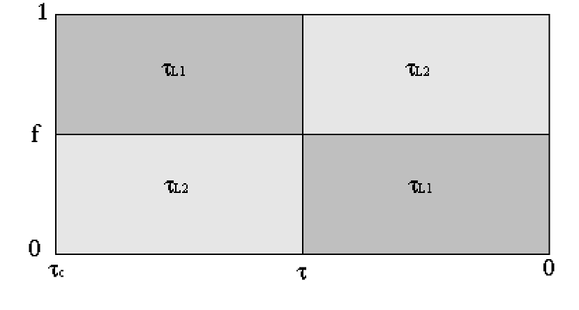
Figure 4: The ionization stratification model. The y-axis represents f-space and the x-axis is measured in units of the continuum optical depth, from $\tau=\tau_{c}$ at the left end to $\tau=0$ at the right end. The radiation from the star enters the wind from the left.

To complete the radiative transfer solution for such an atmosphere, it is necessary to specify the radiation sources. Here we assume pure scattering in radiative equilibrium, but as mentioned above, a key issue is the degree of frequency redistribution per scattering. we assume for simplicity that the continuum opacity scatters coherently. Pinto & Eastman (2000) showed that large amounts of line redistribution have a similar effect on the overall frequency dependent envelope of the radiative flux as does continuum redistribution. We allow the line opacity in one domain to redistribute photons into line opacity in the other domain, using a simple probabilistic approach.

To seek an extreme redistribution limit in such a model is to assert that all line scattering is completely redistributing, so that the probability that any scattering event within a given ionization stratum will be redistributing is

$$\Lambda_{1}\ =\ \frac{\tau_{L1}}{\tau_{L1}+\tau_{c}/2}$$ (38)

for frequency domain 1 and

$$\Lambda_{2}\ =\ \frac{\tau_{L2}}{\tau_{L2}+\tau_{c}/2}$$ (39)

for frequency domain 2, where $\tau_{c}/2$ is the continuum optical depth within a single ionization zone. Thus if the line opacity $\tau_{Li}$ goes to 0, no redistribution may occur in that domain, whereas if $\tau_{Li}$ gets very large, redistribution becomes certain.

However, not all redistribution will result in changing frequency domain, this must be accounted for with a separate probability that obeys the requirement of reciprocity and is independent of the original state of the photon. Thus the probability of redistributing into a particular frequency domain, given that a redistribution has occurred, is

$$w_{1}\ =\ \frac{\tau_{L1}}{\tau_{L1}+\tau_{L2}}$$ (40)

for redistribution into domain 1, and

$$w_{2}=\frac{\tau_{L2}}{\tau_{L1}+\tau_{L2}}$$ (41)

for domain 2. Therefore, the joint probability that a photon will scatter in frequency domain $i$, redistribute, and result in frequency domain $j$ is $\tau_{i}\Lambda_{i}w_{j}$. Note that if $\tau_{Li}$ goes to 0, $w_{i}$ also goes to 0, and no redistribution can occur into that domain. What is less obvious is that if $\tau_{Lj}$ goes to 0, then $w_{i}$ goes to 1, but $\Lambda_{j}=0$, so the joint probability $\Lambda_{j}w_{i}$ of redistributing from frequency domain $j$ into frequency domain $i$, given that a scattering has occured in domain $j$, is still 0.

The fact that eqs. (38)-(41) obey reciprocity may be seen from

$$\frac{p_{12}}{p_{21}}\ =\ \frac{\tau_{1}\Lambda_{1}w_{2}}{\tau_{2}\Lambda_{2}w_{1}}\ =\ 1\ ,$$ (42)

where $p_{ij}$ is the complete probability of scattering in frequency domain $i$ and redistributing into domain $j$. This condition is all that is required for eqs. (38)-(41) to yield the SSR limit if all optical depths are sufficiently large and all gradients are sufficiently gradual. However, it is exactly the impact of more rapid gradients that is being explored by this simple model.

The radiative transport equations that must be solved are

$$\frac{dF_{\ell 1}(\tau)}{d\tau} = 2\frac{\tau_{1}}{\tau_{c}}\Lambda_{1}w_{2}\left(J_{\ell 1}(\tau)-J_{\ell 2}(\tau)\right),$$ (43)

$$\frac{dF_{\ell 2}(\tau)}{d\tau} = 2\frac{\tau_{2}}{\tau_{c}}\Lambda_{2}w_{1}\left(J_{\ell 2}(\tau)-J_{\ell 1}(\tau)\right),$$ (44)

$$\frac{dF_{r1}(\tau)}{d\tau} = 2\frac{\tau_{1}}{\tau_{c}}\Lambda_{1}w_{2}\left(J_{r1}(\tau)-J_{r2}(\tau)\right),$$ (45)

$$\frac{dF_{r2}(\tau)}{d\tau} = 2\frac{\tau_{2}}{\tau_{c}}\Lambda_{2}w_{1}\left(J_{r2}(\tau)-J_{r1}(\tau)\right),$$ (46)

$$\frac{dJ_{\ell 1}(\tau)}{d\tau} = \frac{1}{2}\frac{\tau_{1}}{\tau_{c}}F_{\ell 1}(\tau),$$ (47)

$$\frac{dJ_{\ell 2}(\tau)}{d\tau} = \frac{1}{2}\frac{\tau_{2}}{\tau_{c}}F_{\ell 2}(\tau),$$ (48)

$$\frac{dJ_{r1}(\tau)}{d\tau} = \frac{1}{2}\frac{\tau_{1}}{\tau_{c}}F_{r1}(\tau),$$ (49)

$$\frac{dJ_{r2}(\tau)}{d\tau} = \frac{1}{2}\frac{\tau_{2}}{\tau_{c}}F_{r2}(\tau),$$ (50)

where $\ell$ refers to the left side of the configuration space in Figure 4 and $r$ refers to the right, and 1 denotes the frequency domain that initially contains $\tau_{L1}$ while 2 denotes the frequency domain that initially contains $\tau_{L2}$. These equations may be recast by the following substitutions:

$$x_{\ell}(\tau) \equiv J_{\ell 2}(\tau)-J_{\ell 1}(\tau)\ ,$$ (51)

$$x_{r}(\tau) \equiv J_{r2}(\tau)-J_{r1}(\tau)\ ,$$ (52)

$$y_{\ell}(\tau) \equiv \frac{\tau_{c}}{\tau_{1}}J_{\ell 1}(\tau)+\frac{\tau_{c}}{\tau_{2}}J_{\ell 2}(\tau)\ ,$$ (53)

$$y_{r}(\tau) \equiv \frac{\tau_{c}}{\tau_{1}}J_{r1}(\tau)+\frac{\tau_{c}}{\tau_{2}}J_{r2}(\tau)\ ,$$ (54)

and then eqs. (43)-(50) become

$$\frac{d^{2}x_{\ell}(\tau)}{d\tau^{2}} = ax_{\ell}(\tau)\ ,$$ (55)

$$\frac{d^{2}x_{r}(\tau)}{d\tau^{2}} = ax_{r}(\tau)\ ,$$ (56)

$$\frac{dy_{\ell}(\tau)}{d\tau} = F_{\ell,tot}\ ,$$ (57)

$$\frac{dy_{r}(\tau)}{d\tau} = F_{r,tot}\ ,$$ (58)

where

$$a\ =\ \left(\frac{\tau_{2}}{\tau_{c}}\right)^{2}\Lambda_{2}w_{1}+\left(\frac{\tau_{1}}{\tau_{c}}\right)^{2}\Lambda_{1}w_{2}\ .$$ (59)

The solutions are

$$x_{\ell}(\tau) = C_{\ell+}e^{\sqrt{a}\tau}+C_{\ell-}e^{-\sqrt{a}\tau}\ ,$$ (60)

$$x_{r}(\tau) = C_{r+}e^{\sqrt{a}\tau}+C_{r-}e^{-\sqrt{a}\tau}\ ,$$ (61)

$$y_{\ell}(\tau) = B_{\ell}+F_{\ell,tot}\tau\ ,$$ (62)

$$y_{r}(\tau) = B_{r}+F_{r,tot}\tau\ .$$ (63)

The eight constants $C_{\ell/r,1/2},B_{\ell/r},F_{\ell/r,tot}$ are found by using the following eight boundary conditions: (i) No photons enter the right side of the wind,

$$I_{r-i}(0)=J_{ri}(0)-\frac{1}{2}F_{ri}(0),$$ (64)

where $i$ is 1 or 2, so this represents two boundary conditions. (ii) The fluxes and the mean intensities are continuous at the midpoint of the wind,

$$F_{\ell i}(\tau_{c}/2) = F_{ri}(\tau_{c}/2),$$ (65)

$$J_{\ell i}(\tau_{c}/2) = J_{ri}(\tau_{c}/2),$$ (66)

which gives four more boundary conditions. (iii) The stellar surface at the left of the atmosphere model is assumed to be highly redistributing, so that the incoming intensities on the left are unity,

$$I_{\ell+i}(\tau_{c})=J_{\ell i}(\tau_{c})+\frac{1}{2}F_{\ell i}(\tau_{c})\ =\ 1\ ,$$ (67)

which gives the final two.

Figure 5: The force efficiency as a function of the opacity ratio at $\tau=9$, i.e., one continuum mean-free path from the left edge. The solid lines are the toy model calculations and the dashed lines are the SSR results. The topmost solid and dashed curves are for $\tau_{L1}=10$, the middle are for $\tau_{L1}=20$, and the bottom are for $\tau_{L1}=50$. The asterisks appear where the atmosphere becomes effectively thick to redistribution, i.e. $\tau_{c}=1/\sqrt{a}$, and the crosses appear where all frequency domains become optically thick, i.e., $\tau_{L2}=1$.

Figure 5 shows $\mathcal{E}$ a tenth of the way through the wind, or about a continuum mean-free path from the left edge. The solid lines show the analytic solution, and indicate that there are two circumstances in which a globally gray wind can have a large force efficiency. Not surprisingly, when $\tau_{L1}=\tau_{L2}$, the opacity is truly gray, and $\mathcal{E}=1$. What is more surprising is that as $\tau_{L2}$ is made optically thin, $\mathcal{E}$ also increases, as the flux becomes more gray even though the opacity does not. This is because line emissivity dominates, so the line photons can only be redistributed into other lines. Thus as $\tau_{L2}$ decreases, there are fewer and fewer lines available to receive photons from the thick line region, so in effect the reciprocity condition prevents photons from leaving the thick line region even if that region contains highly redistributing opacity. Indeed, if $\tau_{L2}=0$, then $\mathcal{E}=1$ because no cross-redistribution can occur. This is in stark contrast to the SSR model, which assumes the limit of strong redistribution.

The asterisks in Figure 5 denote the locations in parameter space where the photons thermalize, which can be seen from the exponents of eqs. (60) and (61) to be when $\tau\approx 1/\sqrt{a}$. To the left of the frequency thermalization point, the photons are not efficiently redistributed, so little anti-correlation between flux and opacity is set up, preventing a large drop in $\mathcal{E}$. This drop does appear to the right of the asterisk, where strong frequency thermalization occurs. The crosses denote the locations in parameter space where $\tau_{L2}=1$, which is roughly where the force reaches minimum efficiency. As $\tau_{L2}$ gets larger than 1, the gaps fill in and the wind becomes more gray, allowing a larger $\mathcal{E}$. Thus $\tau_{L2}=1$ is seen as the parameter regime where there is enough line opacity in the thin-line domain to significantly reduce the flux in the thick-line domain, but not enough to achieve multiscattering in the thin-line domain. Thus we find that multiple momentum deposition becomes most difficult whenever the line opacity is distributed such that each ionization zone covers about a single photon mean-free path for a significant flux-weighted fraction of the frequency spectrum. Either less or more nongrayness in the opacity will achieve higher overall force efficiencies.

5.2 Ionization Stratification With Real Line Lists

With the schematic two-domain results in mind, we now return to the real line lists. We have seen that the radiative flux will respond to the opacity as though it was effectively gray over scales much shorter than the frequency thermalization length, which corresponds to some finite range in temperature and may include multiple ionization strata. Over this range, frequency thermalization will take hold and drive the flux toward a coarse-grained version of the SSR limit, so the opacity must be appropriately averaged over the ionization states present. In this picture, the coarse-grained average SSR opacity controls the local flux, which then interacts with truly local opacity to determine the radiative acceleration at each point.

Again, we use the model assumptions in Table 2. The temperature model of LA93, chosen because of its simplicity and emphasis on fundamental processes rather than its completeness relative to more sophisticated models, is used to determine the characteristic maximum range in temperature, some subset of which would correspond to the frequency thermalization length. In their model, the temperature ranges from about $1.35\times 10^{5}K$ at the stellar surface to about $3.5\times 10^{4}K$ at the free-electron photosphere. Without more detailed redistribution calculations (such as carried out by Sim 2004), the appropriate temperature range corresponding to a thermalization depth is unclear, so we consider temperature ranges of $8.0\times 10^{4}K\leq T\leq 1.3\times 10^{5}K$, $6.0\times 10^{4}K\leq T\leq 1.3\times 10^{5}K$, and $4.0\times 10^{4}K\leq T\leq 1.3\times 10^{5}K$ in an effort to span the possibilities. Figures 6, 7, and 8 show the average effective line optical depths from the Kurucz list for these three temperature ranges, respectively. Notice that the gaps begin to fill in as the lower temperature limit reaches $6.0\times 10^{4}K$, and this continues as still lower temperatures are included. However, we do not encounter contributions from a large number of ionization states, in seeming contradiction with LA93 but in agreement with the results of Sim (2004). For example, the latter author found that only two stages of iron have a significant impact on the line-driven mass-loss rate, and this limits the effectiveness of ionization stratification.

5.3 Discussion

Tables 6 and 7 show the effect on the force efficiency and mass-loss rate of including a range in temperatures before applying the SSR flux approximation. The Kurucz list results are again insufficient to describe W-R winds. The OP list results go as high as $8.9\times 10^{-6}M_{\sun}yr^{-1}$. While such mass-loss rates have been observed (Kurosawa et al., 2002), for this to be an upper limit on W-R mass-loss would require large amounts of clumping correction. This mass-loss rate would also require a flux themalization length of about 3 stellar radii to correspond to the required temperature range in the LA93 model, and this seems unrealistically large given the large potential for redistribution found by Pinto & Eastman (2000).

Figure 6: The effective optical depth averaged over the temperature range $8.0\times 10^{4}K\leq T\leq 1.3\times 10^{5}K$.

Figure 7: The effective optical depth averaged over the temperature range $6.0\times 10^{4}K\leq T\leq 1.3\times 10^{5}K$.

Figure 8: The effective optical depth averaged over the temperature range $4.0\times 10^{4}K\leq T\leq 1.3\times 10^{5}K$.

Table 6: Mass-Loss Rates With Ionization Stratification (Kurucz List)

$\Delta T(K)$	$\alpha$	$t$	$M(t)$	$\mathcal{E}$	$a$	$b$	$y_{c}$	$\dot{M}(M_{\sun}yr^{-1})$
$1.3\times 10^{5}-8.0\times 10^{4}$	0.79	0.017	14.5	0.25	32	5.0	1.6	$4.9\times 10^{-6}$
$1.3\times 10^{5}-6.0\times 10^{4}$	0.79	0.018	13.8	0.29	50	4.6	1.8	$5.7\times 10^{-6}$
$1.3\times 10^{5}-4.0\times 10^{4}$	0.80	0.020	12.7	0.34	70	4.3	2.0	$7.1\times 10^{-6}$

Table 7: Mass-Loss Rates With Ionization Stratification (OP List)

$\Delta T(K)$	$\alpha$	$t$	$M(t)$	$\mathcal{E}$	$a$	$b$	$y_{c}$	$\dot{M}(M_{\sun}yr^{-1})$
$1.3\times 10^{5}-8.0\times 10^{4}$	0.72	0.037	13.0	0.24	260	5.2	1.1	$7.6\times 10^{-6}$
$1.3\times 10^{5}-6.0\times 10^{4}$	0.72	0.039	12.5	0.25	260	5.1	1.2	$8.3\times 10^{-6}$
$1.3\times 10^{5}-4.0\times 10^{4}$	0.72	0.041	12.0	0.26	298	4.9	1.2	$8.9\times 10^{-6}$

6 Conclusions

The starting point of this analysis was to recognize that as long as ion thermal speeds are not artificially enhanced by turbulent processes (as considered by Hamann & Grafener, 2004), the Sobolev approximation is entirely applicable to optically thick W-R winds. Thus CAK theory is applicable after modifying for the effects of diffuse radiation on the ionization and the angle dependence of the radiative flux, and it is found that lines are able to drive abundant mass loss under hot W-R plasma conditions. However, the ubiquitous presence of frequency redistribution in an optically thic flow introduces significant challenges to achieving large line-driven W-R mass-loss rates, and so the rate of frequency thermalization is critical for quantifying how redistribution affects the efficiency of line driving.

With rapid enough thermalization, the radiative flux avoids large opacity domains, resulting in force efficiencies well below what is needed to drive the observed W-R mass-loss rates. This drop in force efficiency in a highly redistributing optically thick wind may only be avoided by filling the gaps locally, which requires the discovery of new lines in regions of the spectrum that are less densely packed. Our test calculation demonstrated that the greatest challenge to driving efficiency is presented by spectral domains in which optically thick lines barely overlap over the wind terminal speed, since regions where the lines are sparse are less likely to be redistributed into, and regions where the lines are dense are already effective at line driving.

If, on the other hand, the thermalization rate is slow enough to sample a wide range in ionization strata, then gray-type force efficiencies may in principle be recovered. However, in practice the line lists do not appear to exhibit sufficiently rich contributions from the many different ionization states to achieve widespread filling-in of the spectrum. As a result, frequency redistribution into domains with relatively little line overlap continues to present a severe challenge to obtaining line-driven winds with large frequency-averaged optical depth, as would be required to attain the largest of the Wolf-Rayet mass-loss rates inferred from observations. In short, there still does not exist a priori opacity-driven models of supersonically accelerating optically thick winds with low turbulent broadening and non-static opacity treatments that can explain how a smaller and hotter W-R star can have a dramatically enhanced mass-loss rate. Either the opacity is still incomplete and new lines are capable of filling in the line-poor domains, or else clumping corrections reduce the need for W-R mass fluxes to substantially exceed those of their cooler, larger, and H-rich cousins, the extreme Of stars.

In addition, it should be noted that up-to-date opacity treatments from the Opacity Project (Badnell & Seaton, 2003) and the OPAL opacity tables (Rogers & Iglesias, 1992) are of static type so are not in their purest form applicable to W-R winds. They must first be re-evaluated as expansion-type opacities, such as the method of Jeffery (1995) or the SSR mean used here, possibly also incorporating more exact radiative transfer (Pinto & Eastman, 2000) or non-Sobolev opacity corrections (Wehrse et al., 2003), before they may be appropriately applied to further investigations into the role of high-temperature opacity contributions (such as the “iron bump”) in explaining high W-R mass fluxes. Furthermore, the critical point must not be artificially placed in regions of exceptionally high opacity, as this would belie the meaning of the critical point as the “choke point” of wind acceleration.‘

It must also be mentioned that although clumping corrections reduce both the inferred W-R mass-loss rates and the difficulty in explaining them with existing line opacities, clumping itself may introduce dynamical challenges. This is not a problem for clumps smaller than the Sobolev length $L$, but larger clumps will reduce the force efficiency in ways that are classifiable according to whether the clumps are optically thin or thick to most photons. When the clumps are thin, their impact is felt only through the role of density and velocity in standard CAK theory, but when the clumps are thick (e.g., Brown et al., 2004), additional reductions in the force efficiency must appear owing to the feedback onto the self-consistent radiative flux, in a manner again similar to the spirit of a Rosseland mean (Owocki et al., 2004). The development and dynamical implications of such clumps require detailed radiation hydrodynamic simulations, but the simplified approaches developed here may be used to guide approximations that make such a time-dependent calculation (e.g., Baron & Hauschildt, 2004; Gräfener & Hamann, 2005) computationally tractable.

Finally, the most important goal of this paper has been to develop a conceptual vocabulary to discuss the circumstances under which a W-R wind may or may not be efficiently driven by Sobolev-type line opacity. Key elements of this vocabulary include the effectively gray optical depth $\tau_{g}$, the nongray force efficiency $\mathrel{E}$, the nongrayness parameter $b$ for the monotonically reordered line distribution, and the range of ionization strata that contribute within a photon frequency thermalization length. Estimations of these parameters offer conceptual insights into classifying various physical behaviors, both before and after carrying out optically thick radiation hydrodynamical simulations.

References

- Badnell & Seaton (2003) Badnell, N. R. & Seaton, M. J. 2003, J. Phys. B, 36, 4367
- Barlowe et al. (1981) Barlowe, M. J., Smith, L. J., & Willis, A. J. 1981, MNRAS, 196, 101
- Baron & Hauschildt (2004) Baron, E. & Hauschildt, P. H. 2004, A&A, 427, 987
- Brown et al. (2004) Brown, J. C., Cassinelli, J. P., Li, Q., Kholtygin, A. F., & Ignace, R. 2004, A&A, 426, 323
- Cassinelli & van der Hucht (1987) Cassinelli, J. P. & van der Hucht, K. A. 1987, in Instabilities in Luminous Early Type Stars, ed. H. J. G. Lamers & C. W. H. De Loore, Astrophysics and Space Science Library (Dordrecht: Reidel), 136, 231
- Castor et al. (1975) Castor, J. I., Abbott, D. C., & Klein, R. I. 1975, ApJ, 195, 157
- Crowther et al. (2002) Crowther, P. A., Dessart, L., Hillier, D. J., Abbott, J. B., & Fullerton, A. W. 2002, A&A, 392, 653
- De Marco et al. (2000) De Marco, O., Schmutz, W., Crowther, P. A., Hillier, D. J., Dessart, L., de Koter, A., & Schweickhardt, J. 2000, A&A, 358, 187
- Friend & Castor (1983) Friend, D. B., & Castor, J. I. 1983, ApJ, 272, 259
- Gayley et al. (1995) Gayley, K. G., Owocki, S. P., & Cranmer, S. R. 1995, ApJ, 442, 296
- Gräfener & Hamann (2005) Gräfener, G., & Hamann, W.-R. 2005, A&A, 432, 633
- Hamann & Grafener (2004) Hamann, W.-R. & Grafener, G. 2004, A&A, 427, 697
- Herald et al. (2000) Herald, J. E., Schulte-Ladbeck, R. E., Eenens, P. R. J. & Morris, P. 2000, ApJS, 126, 469
- Hillier & Miller (1999) Hiller, D. J. & Miller, D. L. 1999, ApJ, 519, 354
- Hillier (2003) Hillier, D. J. 2003, IAU Symposium, 212, 70
- Jeffery (1995) Jeffery, D. J. 1995, A&A, 299, 770
- Kurosawa et al. (2002) Kurosawa, R., Hillier, D. J., & Pittard, J. M. 2002, A&A, 388, 957
- Kurucz (1979) Kurucz, R. L. 1979, ApJS, 40, 1
- Lucy & Abbott (1993) Lucy, L. B. & Abbott, D. C. 1993, ApJ, 405, 738 (LA93)
- Morris et al. (2000) Morris, P. W., van der Hucht, K. A., Crowther, P. A., Hillier, D. J., Dessart, L., Williams, P. M., & Willis, A. J. 2000, A&A, 353, 624
- Nugis et al. (1998) Nugis, T., Crowther, P. A., & Willis, A. J. 1998, A&A, 333, 956
- Nugis & Lamers (2000) Nugis, T. & Lamers, H. J. G. L. M. 2000, A&A, 360, 227
- Nugis & Lamers (2002) Nugis, T., & Lamers, H. J. G. L. M. 2002, A&A, 389, 162
- Onifer & Gayley (2003) Onifer, A. J. & Gayley, K. G. 2003, ApJ, 590, 473
- Owocki et al. (2004) Owocki, S. P., Gayley, K. G., & Shaviv, N. J. 2004, ApJ, 616, 525
- Pinto & Eastman (2000) Pinto, P. A. & Eastman, R. G. 2000, ApJ, 530, 757
- Rogers & Iglesias (1992) Rogers, F. J. & Iglesias, C. A. 1992, ApJS, 79, 507
- Sim (2004) Sim, S. A. 2004, MNRAS, 349, 899
- Springmann (1994) Springmann, U. 1994, A&A, 289, 505
- Springmann & Puls (1995) Springmann, U. & Puls, J. 1995, IAU Symposium, 163, 170
- Wehrse et al. (2003) Wehrse, R., Baschek, B., & von Waldenfels, W. 2003, A&A, 401, 43