Disk eccentricity and embedded planets

Abstract

Aims. We investigate the response of an accretion disk to the presence of a perturbing protoplanet embedded in the disk through time dependent hydrodynamical simulations.

Methods. The disk is treated as a two-dimensional viscous fluid and the planet is kept on a fixed orbit. We run a set of simulations varying the planet mass, and the viscosity and temperature of the disk. All runs are followed until they reach a quasi-equilibrium state.

Results. We find that for planetary masses above a certain minimum mass, already $3M_{Jup}$ for a viscosity of $\nu=10^{-5}$, the disk makes a transition from a nearly circular state into an eccentric state. Increasing the planetary mass leads to a saturation of disk eccentricity with a maximum value of around 0.25. The transition to the eccentric state is driven by the excitation of an $m=2$ spiral wave at the outer 1:3 Lindblad resonance. The effect occurs only if the planetary masses are large enough to clear a sufficiently wide and deep gap to reduce the damping effect of the outer 1:2 Lindblad resonance. An increase in viscosity and temperature in the disk, which both tend to close the gap, have an adverse influence on the disk eccentricity.

Conclusions. In the eccentric state the mass accretion rate onto the planet is greatly enhanced, an effect that may ease the formation of massive planets beyond about 5 $M_{Jup}$ that are otherwise difficult to reach.

1 Introduction

In the early stages of their formation protoplanets are still embedded in the disk from which they form. Not only will the protoplanet accrete material from the disk and increase its mass, it will also interact gravitationally with it. Planet-disk interaction is an important aspect of planet formation because it leads to a change in the planetary orbital elements. Already before the discovery of extrasolar planets the interaction of an embedded object with a disk has been studied for small perturber masses by linear analysis (eg. Goldreich & Tremaine 1980; Papaloizou & Lin 1984; Ward 1986), and in more recent years also for massive planets through detailed numerical simulations in two and three dimensions (eg. Bryden et al. 1999; Kley 1999; Kley et al. 2001; D’Angelo et al. 2002; Bate et al. 2003). In all these simulations the planet has been held fixed on a circular orbit and its influence onto the disk has been analyzed. The back reaction of the disk in terms of migration rate or eccentricity change can be calculated by summing over the force contribution of each disk element.

The full evolution of a single planet embedded in a disk has been followed for example by Nelson et al. (2000). In a later study by Papaloizou et al. (2001) numerical simulations have been performed for a range of planetary masses with emphasis on the eccentricity evolution of the planets. It has been found that massive planets create an eccentric disturbance in the outer disk which in turn may back-react on the planet and increase its eccentricity. However, only for planets larger than 10-20 Jupiter masses a visible increase up to $e=0.20$ has been found. However, these values are significantly below the observed eccentricities for extrasolar planets which average at about $e=0.3-0.4$ for planetary masses between 1 and 10 $M_{Jup}$. Also for smaller planet masses an average eccentricity of about $e=0.3$ is observed. This may be due to planet-planet interactions, but these interactions are more effective with increasing planet mass. For a recent overview of planetary properties see Marcy et al. (2005) and the Extrasolar Planets Encyclopedia (http://www.obspm.fr/encycl/encycl.html) maintained by J. Schneider. The distribution of eccentricities does not show a strong dependence on $m\sin{i}$ nor on the distance from the central star.

As one possible scenario to explain the origin of the observed high eccentricities the aforementioned interaction of a planet with the protoplanetary disk has been suggested. In particular, Goldreich & Sari (2003); Sari & Goldreich (2004) estimate that Lindblad resonances may lead to eccentricity growth under reasonable assumptions. Numerical simulations tend to show the opposite, for Jupiter mass planets the eccentricity is typically damped on short time scales $\approx 100$ orbits, only for massive planets at least transient growth has been seen (Nelson et al. 2000). This last result may be related to the back reaction of an eccentric disk onto the planet, where the disk’s eccentricity has been induced by the presence of the massive planet. Additionally, the mass of the embedded planet has also profound consequences for the mass accretion rate onto it, i.e. its growth-time. As the induced gap in the disk becomes wider and deeper upon increasing $M_{p}$ the accretion rate diminishes and essentially limits the growth for masses beyond 5 $M_{Jup}$ (Bryden et al. 1999; Lubow et al. 1999). However, those calculations covered only a couple of hundred orbits of the planet which is much smaller than the viscous time scale. Consequently, no equilibrium structure has been reached.

Here we follow this line of thought and investigate the influence a massive embedded planet has on the structure of the ambient protoplanetary disk. We use a hydrodynamical description to follow the evolution of the disk, where the planet is fixed on a circular or a slightly eccentric orbit. All simulations are run until a quasi-stationary equilibrium has been reached and overall values of mass and energy in the computational domain remain unchanged. We vary the mass of the planet, the temperature and the disk viscosity, and analyze their influence on the structure of the disk, in particular on its eccentricity. Indeed, we find that (for a given viscosity) there appears to be clear transition in the disk from an circular state into an eccentric state.

We analyze the magnitude of the induced disk eccentricity and estimate its influence on the accretion rate of the planet. In particular, we find that for sufficiently massive planets the disk becomes eccentric, where the critical minimum mass depends on the value of the viscosity coefficient.

For a viscosity of $\alpha=4\times 10^{-3}$, a reasonable value for protoplanetary disks, the disk becomes eccentric already for planets of 3 Jupiter masses. At the same time the mass accretion rate onto the planet increases strongly for an eccentric disk.

In the next section we describe our model assumptions, in section 3 we present our results followed by theoretical analysis and conclusions.

2 The Standard Hydrodynamical Model

The models presented here are calculated basically in the same manner as those described previously in Kley (1998, 1999). The reader is referred to those papers for details on the computational aspects of this type of simulations. Other similar models, following explicitly the motion of single planets in disks, have been presented by Nelson et al. (2000), Bryden et al. (2000).

We use cylindrical coordinates ($r,\varphi,z$) and consider a vertically averaged, infinitesimally thin disk located at $z=0$. The origin of the coordinate system, which is co-rotating with the planet, is either at the position of the star or in the combined center of mass of star and planet. Since in the first case the coordinate system is accelerated and rotating, care has to be taken to include also the indirect terms of the acceleration (Kley 1998). The basic hydrodynamic equations (mass and momentum conservation) describing the time evolution of such a viscous two-dimensional disk with embedded planets have been stated frequently and are not repeated here (see Kley 1999).

In the present study we restrict ourselves to the situation where the embedded planet is on a fixed orbit, i.e. the gravitational back reaction of the disk on the planet is not taken into account.

2.1 Initial Setup

The two-dimensional ($r-\varphi$) computational domain consists of a complete ring of the protoplanetary disk. The radial extent of the computational domain (ranging from $r_{\mathrm{min}}$ to $r_{\mathrm{max}}$) is taken such that there is enough space on both sides of the planet, although, as we shall see later, the effect we are analyzing appears to occur only in the outer disk. Typically, we assume $r_{\mathrm{min}}=0.40$ and for $r_{\mathrm{max}}$ we take two different values 2.5 and 4.0, in units where the planet is located at $r=1$. In the azimuthal direction for a complete annulus we have $\varphi_{\mathrm{min}}=0$ and $\varphi_{\mathrm{max}}=2\pi$.

The initial hydrodynamic structure of the disk (density, temperature, velocity) is axisymmetric with respect to the location of the star. The surface density is constant ($\Sigma=1$ in dimensionless units) over the entire domain with no initial gap. To make sure that only little disturbances or numerical artifacts arise upon immersion of the planet, its mass will be slowly turned on from zero to the final required mass (eg. 5 Jupiter masses) over a time span of typically 50 orbital periods. The initial velocity is pure Keplerian rotation ($u_{r}=0,u_{\varphi}=\Omega_{K}r=(GM_{*}/r)^{1/2}$), and the temperature stratification is always given by $T(r)\propto r^{-1}$ which follows from an assumed constant vertical height $H/r$. For these isothermal models the temperature profile is left unchanged at its initial state throughout the computations.

For our standard model we use a constant kinematic viscosity coefficient $\nu$ but present additionally a sequence of $\alpha$-disk models.

2.2 Boundary conditions

To ensure a most uniform environment for all models and minimize disturbances (wave reflections) from the outer boundary we impose at $r_{\mathrm{min}}$ and $r_{\mathrm{max}}$ damping boundary conditions where the density and both velocity components are relaxed towards their initial values as

$$\frac{dX}{dt}=-\frac{X-X(t=0)}{\tau_{\mathrm{damp}}}\,R(r)^{2}$$ (1)

where $X\in\{\Sigma,u_{r},u_{\varphi}\}$, $\tau_{\mathrm{damp}}=1/\Omega_{\mathrm{K}}(r_{\mathrm{boundary}})$ and $R(r)$ is a dimensionless linear ramp-function rising from 0 to 1 from $r_{\mathrm{damp}}$ to $r_{\mathrm{boundary}}$. Here, $r_{\mathrm{boundary}}$ is either $r_{\mathrm{min}}$ or $r_{\mathrm{max}}$, depending which edge of the disk is considered. The initial radial velocity vanishes, and the boundary conditions ensure that no mass flows through the radial boundaries at $r_{\mathrm{min}}$ and $r_{\mathrm{max}}$. However, the total mass in the system may nevertheless vary due to the applied damping. In the azimuthal direction, periodic boundary conditions for all variables are imposed.

These specific boundary conditions allow upon a long term evolution for a well defined quasi-stationary state if there is no back-reaction of the disk on the orbital elements of the planet.

2.3 Model parameters

The computational domain is covered by 128 $\times$ 384 ($N_{r}\times N_{\varphi}$) grid cells for the smaller models $[0.4,2.5]$ and $200\times 384$ for the larger $[0.4,4.0]$ ones. The grid is spaced equidistant in both radius and azimuth. The inner radius beyond which the damping procedure defined above gradually sets in is given by $r_{\mathrm{damp}}=0.5$, the outer damping radius is given by $R_{\mathrm{damp}}=0.84r_{\mathrm{max}}$. The star has a mass of 1 $M_{\odot}$, and the mass of the planet in the different models ranges from one to five Jupiter masses. The planet is held on a fixed circular orbit.

For the viscosity a value of $\nu=1.0\cdot 10^{-5}$ (in units of $\Omega_{p}r_{p}^{2}$) is used for our standard models, which is equivalent to a value of $\alpha=0.004$ for the standard $H/r=0.05$. This is a typical value for the effective viscosity in a protoplanetary disk.

To achieve a more detailed calculation of the observed phenomena we refined some calculations to the higher resolution of 260 x 760 ($N_{r}\times N_{\varphi}$) by interpolating the data from coarser calculations. As the relaxation time for the system is very long ($>$ 1000 orbits) it would be too time-consuming to complete the whole calculation on the high-resolution grid. These higher resolution simulations yield identical results. To study the influence of physical parameters such as viscosity and pressure, we vary $\nu$ and $H/r$ in some models. In addition, we analyze the influence of several numerical parameters on the results.

2.4 A few remarks on numerical issues

We use two different codes for our calculations, RH2D and NIRVANA. The numerical method used in both codes is a staggered mesh, spatially second order finite difference method based, where advection is based on the monotonic transport algorithm (van Leer 1977). Due to operator-splitting the codes are semi-second order in time. The computational details of RH2D which can be used in different coordinate systems have been described in general in Kley (1989), and specifically for planet calculations in Kley (1999). The details of the NIRVANA code have been described in Ziegler (1998).

The use of a rotating coordinate system requires special treatment of the Coriolis terms to ensure angular momentum conservation (Kley 1998). Especially for the long-term calculations presented here, this is an important issue.

In calculating the gravitational potential of the planet we use a smoothed potential of the form

$$\Phi_{P}=-\frac{GM_{\mathrm{p}}}{\sqrt{s^{2}+\epsilon^{2}}}$$ (2)

where $s$ is the distance from the planet. For the smoothing length of the potential we choose $\epsilon=0.4R_{\mathrm{Hill}}$.

The viscous terms, including all necessary tensor components, are treated explicitly. To ensure stability in the gap region with very strong gradients in the density an artificial bulk viscosity has been added, with a coefficient $C_{\mathrm{art}}=1.0$. For the detailed formulation of the viscosity related issues and tests see Kley (1999).

As the mass ratio $M_{\mathrm{p}}/M_{*}$ of the planet can be very large we have found it preferable to work with a density floor, where the density cannot fall below a specified minimum value $\Sigma_{\mathrm{min}}$. For our purpose we use a value of $\Sigma_{\mathrm{min}}=10^{-8}$ in dimensionless values, where the initial density is of ${\cal{O}}(1)$.

3 The dual-state disk

We first consider our standard model as described above using a planetary mass ranging from 1 to 5 $M_{Jup}$, i.e. a mass ratio of $q=10^{-3}$ to $5\cdot 10^{-3}$. The other physical parameters are identical for all models. Due to the nature of the damped boundary conditions and a non-zero physical viscosity we might expect after a sufficiently long evolution time a convergence towards an equilibrium state where the density structure and the total amount of mass in the disk remain constant in time, at least in the co-rotating frame. Indeed, for small planetary masses, $M_{p}<3M_{Jup}$ we find a circular stationary state which displays the typical features of embedded planets in disks: a deep, circular depression of density at the location of the planet (the gap), spiral arms in the inner and outer disk. This state is shown in the top graph of Fig. 1, which shows the surface density of the obtained equilibrium state at an evolutionary time of $t=2000$ orbits.

However, if the planetary mass reaches $M_{p}\geq 3M_{Jup}$ we surprisingly do not reach a stationary equilibrium state anymore. Instead we find after a very long time ($>1000$ orbits) a new periodic state which has approximately the same period as the orbital period of the planet. In this state the disk is clearly eccentric with an extremely slow precession rate such that the eccentric pattern appears to be nearly stationary in the inertial frame. This eccentric quasi-equilibrium state for $M_{\mathrm{p}}=5M_{Jup}$ is shown in the bottom graph of Fig. 1.

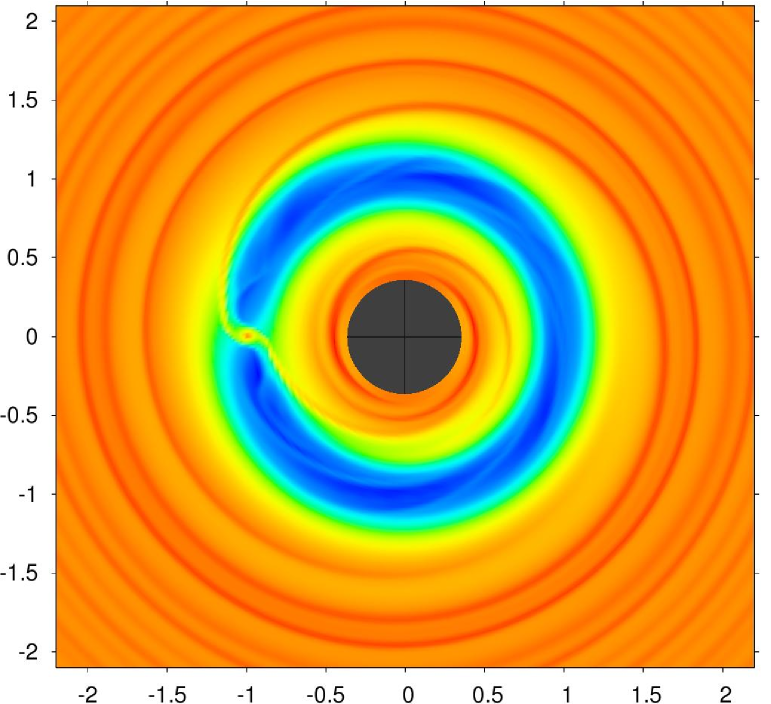
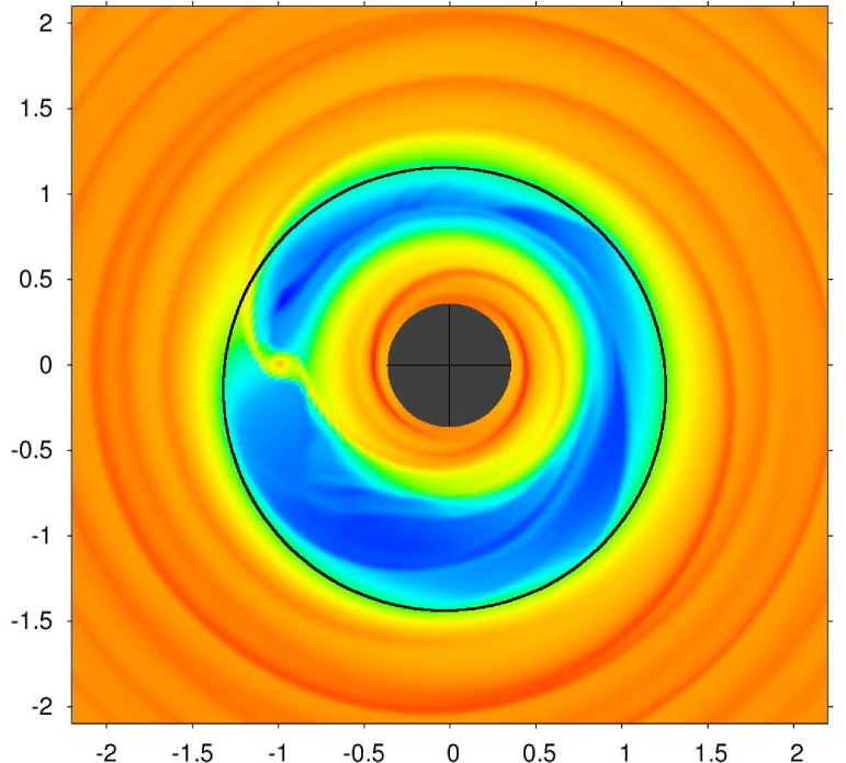
Figure 1: Logarithmic plots of the surface density $\Sigma$ for the relaxed state after 2000 orbits for two different masses of the planet which is located at $r=1.0$ in dimensionless units. Top) $q=3.0\,10^{-3}$ and Bottom) $q=5.0\,10^{-3}$ calculated with NIRVANA. The inner disk stays circular in both cases but the outer disk only in the lower mass case. For $q=5.0\,10^{-3}$ it becomes clearly eccentric with some visible fine structure in the gap. For illustration, the drawn ellipse (solid line in the lower plot) has one focus at the stellar location and an eccentricity of 0.20.

3.1 The eccentric disk

A measure of the eccentricity of the disk is calculated as follows: For a ring at radius $r_{i}$ we calculate the eccentricity for every cell in the ring from the velocity and position vector of that cell by assuming the fluid element is a particle moving freely in the central potential of the star, feeling no pressure forces. The average over all cells in the ring is then defined as the eccentricity of the disk at that radius $r_{i}$. This value is plotted for different masses in Fig. 2 at the evolutionary time of $t=2500$, only for $M_{p}=3M_{Jup}$ at $t=3850$ orbits.

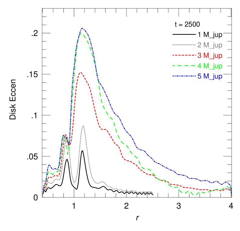
Figure 2: Disk eccentricity as a function of radius for the several models with $q=0.001$ up to $q=0.005$ at $t=2500$ orbits, for the $q=0.003$ model at $t=3850$. For the two lower curves $q=0.001$ and $q=0.002$, the outer edge of the computational domain lies at $r_{max}=2.5$.

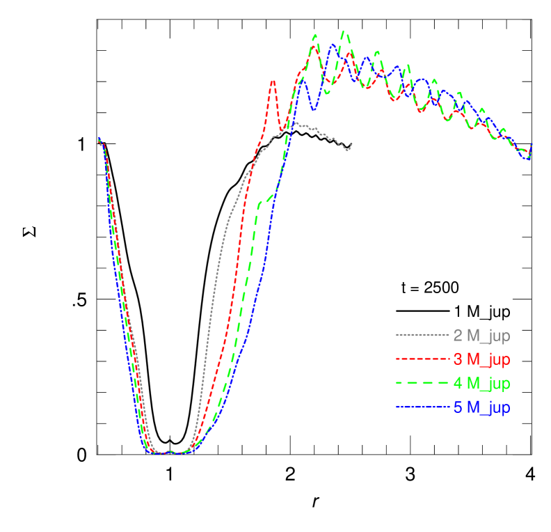
Figure 3: Azimuthally averaged radial profiles of the surface density for different planet masses, for the same models and times as in Fig. 2. The width of the gap increases with planetary mass.

For planetary masses below around $M_{p}\approx 3M_{Jup}$, the maximum eccentricity of the disk is about 0.10, and is strongly peaked at $r\approx 1.2$. For the larger planetary masses the eccentricity of the disk nearly doubles and reaches 0.22 for $M_{p}=5M_{Jup}$. In addition, a much larger region of the disk has become eccentric, which has been seen clearly already in the surface density distribution in Fig. 1, bottom, where the ellipse indicates an eccentricity of 0.20 with one focus at the stellar position. The precession rate $\dot{\varpi}$ of the eccentric disk is very small and typically prograde. From our longest runs (over several thousand orbits) we estimate $\dot{\varpi}\approx 10\deg/1000$ Orbits. In Fig. 2 the curves for the lower planet masses end at $r=2.5$ because this is the outer boundary for those low mass models.

In Fig. 3 the azimuthally averaged density profile is plotted for different planetary masses for the same models as in Fig. 2. Clearly the gap width increases for the larger planet mass, as expected due to the stronger gravitational torques. For the lowest mass $q=0.001$ model (solid line) the gap is not completely cleared.

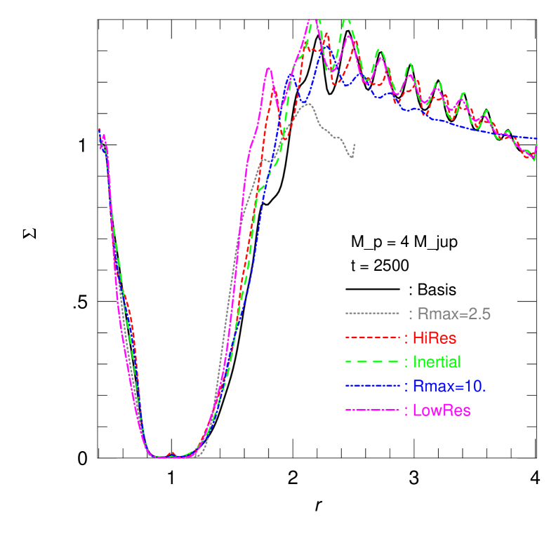
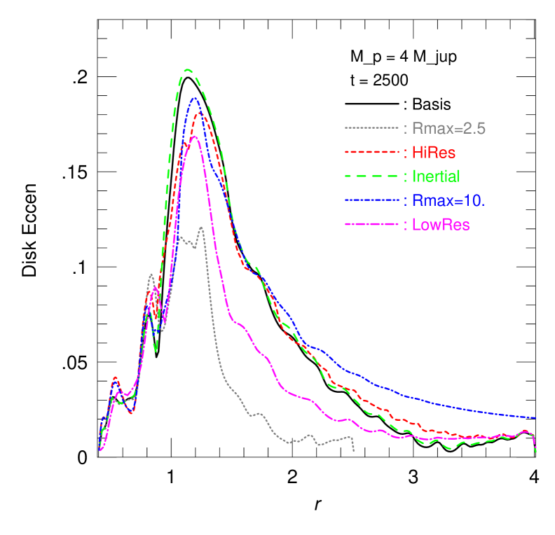
Figure 4: Surface density and eccentricity profile for models using $q=0.004$ at a time of 2500 orbits, the high resolution (model short dashed line) at 1750 orbits. Plotted are results for different models varying the numerical setup.

3.2 Dependencies on numerical parameters

The threshold mass where the transition from circular to eccentric occurs apparently depends on the width and shape of the gap, and parameters that will change the gap structure will also change this threshold mass. Before we analyze physical influences we display in Fig. 4 the surface density profile and the disk eccentricity for models using different numerical parameters but all with same physical setup for $q=0.004$, and at the same evolutionary time of 2500 orbits (the high resolution model at $t=1750$ orbits).

The solid line refers to the basic reference model (as in Fig. 3, $4M_{Jup}$ model). We first find that the mass value where the transition occurs may depend on the location of the outer boundary $r_{\mathrm{max}}$. If the stand-off distance of the planet to the outer boundary is too small the damping boundary conditions, which tend to circularize the disk, prevent the disk from becoming eccentric. The simulations using a $4M_{Jup}$ planet and a smaller $r_{\mathrm{max}}$ clearly shows this effect. For this mass of the planet the disk will not anymore become eccentric for $r_{\mathrm{max}}=2.5$ (dotted curve). Hence, to properly study this effect a sufficiently large $r_{max}$ has to be chosen. An extended domain with $r_{\mathrm{max}}=10$ (short-dashed-dotted) does not alter the eccentricity behavior of the disk. The inner disk remains circular for all planet masses because of the strong damping introduced by the boundary condition.

A higher resolution (200 $\times$ 500, short-dashed line), and running the model in the inertial frame (long-dashed) have no significant influence on the density distribution and the occurrence and magnitude of the disk eccentricity. A lower resolution model (long-dashed-dotted) using 128 $\times$ 128 grid cells, results in a slightly lower eccentricity due to a larger (numerical) damping. In addition, we have compared results with two different numerical codes (RH2D and NIRVANA) and again found good agreement. Hence, we conclude that the eccentric disk state is a robust, reproducible physical phenomenon.

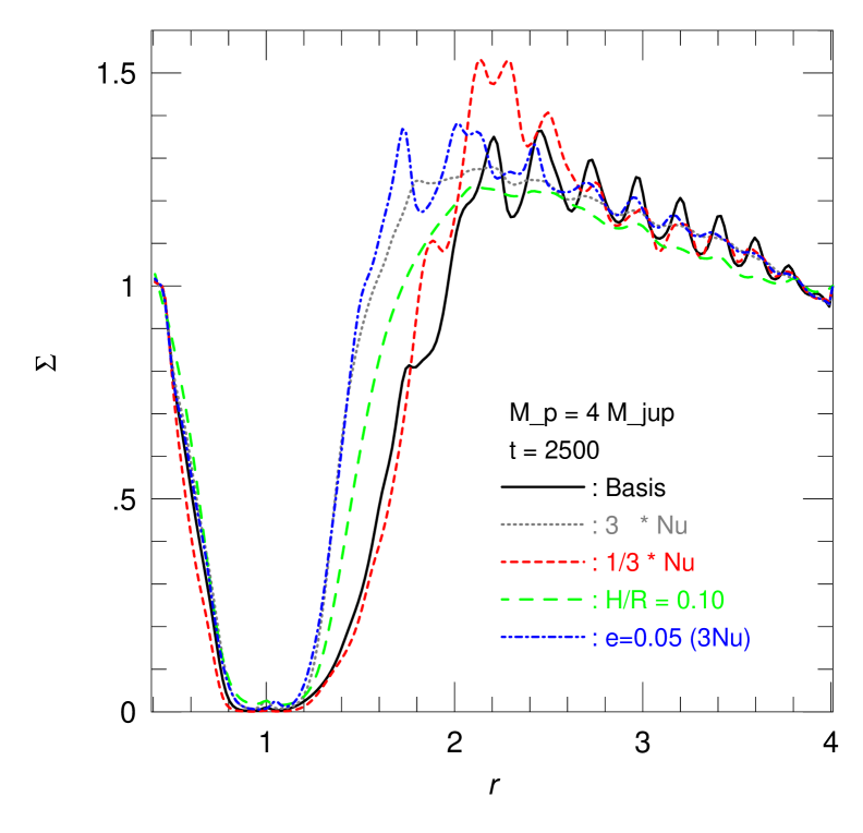
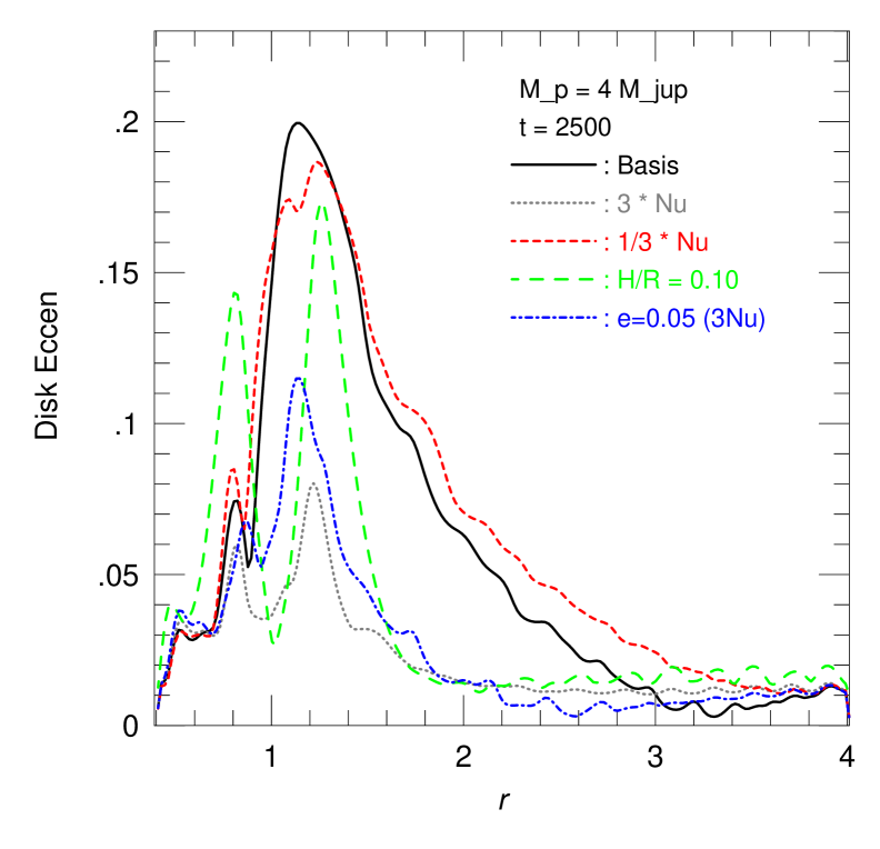
Figure 5: Surface density and eccentricity profile for models using $q=0.004$ at a time of 2500 orbits. Plotted are results for different models varying the physical setup.

3.3 Dependencies on physical parameters

In Fig. 5 we display the surface density profile and the disk eccentricity for models with $q=0.004$ using different physical parameters. If the dimensionless viscosity $\nu$ is enlarged to $3\times 10^{-5}$ (dotted line) the gap width and depth is reduced and the disk will no longer become eccentric for the planet mass of $q=0.004$ (and also not for $q=0.005$). Similarly, an increased $H/r$ (long-dashed line) leads also to a narrower gap and a smaller disk eccentricity. If, on the other hand, the viscosity is lowered by a factor of three (short-dashed), or $H/r$ is reduced we find that the disk reaches about the same eccentricity as before.

The last model (dashed-dotted line) refers to a planet on an eccentric orbit with $e_{p}=0.05$ and a 3 times higher viscosity than the basis model. As can be seen, the disk remains circular for these parameter. This model demonstrates that it is not the planetary eccentricity which is responsible for producing the disk eccentricity but that it is rather a genuine instability. This conclusion is confirmed by a model with $M_{p}=2M_{Jup}$ and $e_{p}=0.05$ which (for the standard viscosity) does not produce an eccentric disk.

3.4 The two equilibrium states for an $\alpha$ type viscosity

To illustrate the effect under different physical conditions we present additional simulations using a slightly different setup. Here, we consider a planet moving inside a disk at a radius of 0.35 AU, assuming that the inner disk has been cleared already. The outer radius of the computational domain lies at 1.2 AU, and the inner one at 0.25 AU. The scale height of the disk is $H/r=0.05$, and for the viscosity we use here as an alternative an $\alpha$-prescription, with a constant value of $\alpha=0.01$. In these models we have used a planetary eccentricity of $e_{p}=0.01$ which is typically found in models of embedded planets that follow the orbital evolution. As shown above this value of $e_{p}$ has no influence on the transition to the eccentric disk state. The remaining setup is similar to the models described above. The viscosity may be on the large side of protoplanetary disks but has (in combination with the lack of the inner disk) the clear advantage of speeding up the simulations considerably which allows us to reach the quasi-equilibrium states in which global quantities such as mass, energy do not vary in time anymore, with reasonable computational effort. This alternative setup has been used recently in a paper modeling the resonant system GJ 876 and it is described in more detail in Kley et al. (2005). Here we describe additional results concerning details of the eccentric disk state.

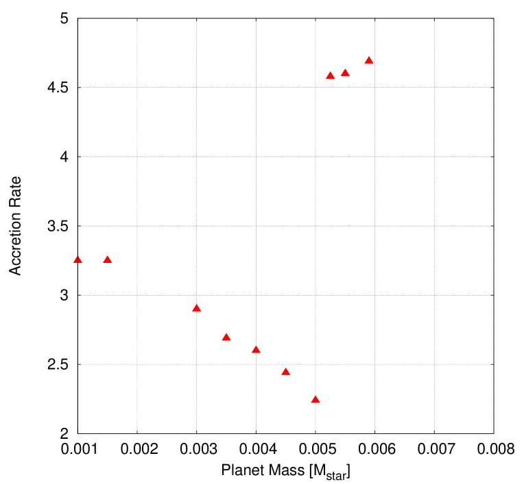
Figure 6: The dependence of the accretions rate onto the planet (in dimensionless units) on the planetary mass for relaxed quasi-equilibrium configurations. Results are displayed for models using an $\alpha=0.01$ viscosity.

For these $\alpha$-models we vary the planet-star mass ratio $q$ from $1\cdot 10^{-3}$ to about $7\cdot 10^{-3}$. In all cases the models are evolved until a quasi-stationary state has been reached. As already seen above for the constant viscosity case, also in this case the disk changes its structure from circular for small planetary masses to eccentric for large planetary masses. Here the transition occurs at a larger planetary mass because of the higher effective viscosity.

In Fig. 6 we display the mass accretion rate onto the planet as a function of the planet mass. There is a strong jump in the magnitude of the accretion rate at a critical planetary mass $q_{crit}\approx 5.25\cdot 10^{-3}$, exactly at the point where the disk switches from circular to eccentric. For small planetary masses $q<q_{crit}$ the mass accretion rate falls off with increasing planetary mass, because upon increasing $M_{p}$ the stronger gravitational torques will deepen the gap and reduce the accretion rate (Bryden et al. 1999; Lubow et al. 1999). However, when the disk turns eccentric the gap edge periodically approaches the planet and it may even become engulfed in the disk material for sufficiently large eccentricity (see Fig. 7). Consequently, the mass accretion rate onto the planet is strongly increased allowing for more massive planets.

This sudden change in the accretion rate is reminiscent of a phase transition where the ordering parameter is given here by the planetary mass. Test simulations have shown that the obtained equilibrium structure does not depend on the initial configuration (eg. density profile, initial mass in the disk) but is solely given by the chosen physical parameters. As shown above the transition from the non-eccentric state to the eccentric state, which is here a function of only the planetary mass, depends also on the viscosity and temperature on the disk which we have held fixed in this model sequence.

Similarly to accretion rate the total disk mass contained in the system also changes abruptly at the $q_{crit}$ as a consequence of the applied the boundary conditions at $r_{max}$. These are chosen such that the disk relaxes towards its initial conditions at the outer boundary, eg. the value of the surface density is fixed at that point. Upon increasing the planet mass the gap becomes more pronounced and disk mass is pushed towards the outer boundary increasing the density there. At the onset of the eccentric state this relation changes abruptly.

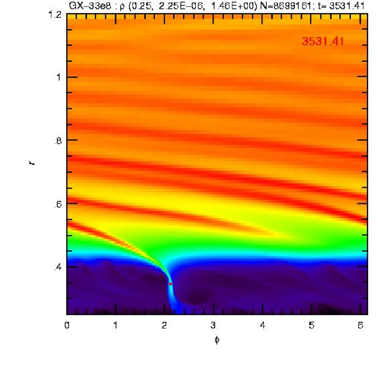
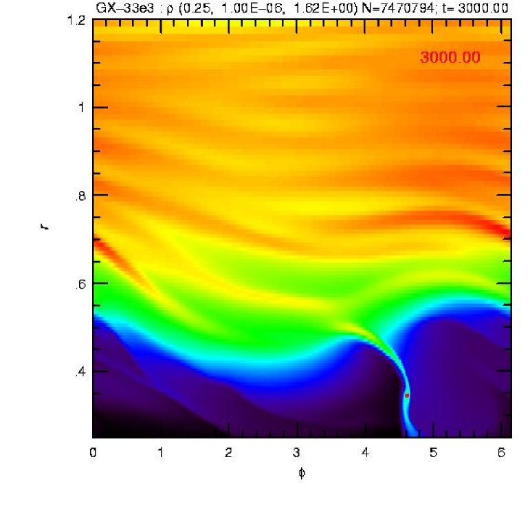
Figure 7: Gray scale plots of the surface density $\Sigma$ for the relaxed state for two different planetary masses: a) $q=4.5\cdot 10^{-3}$ and b) $q=5.9\cdot 10^{-3}$ calculated with RH2D. Due to the higher planetary mass much stronger wave-like disturbances are created in the density.

The existence of the two equilibrium states of the disk is further illustrated in Fig. 7 where we display gray scale plots of the surface density $\Sigma$ for the relaxed state. for two different mass ratios ($q=4.5$ and $5.9\cdot 10^{-3}$) in a $r-\varphi$ representation. While for the lower mass case ($q=4.5\cdot 10^{-3}$) the disk structure remains quite regular, the second high mass case ($q=5.9\cdot 10^{-3}$) shows a strongly disturbed disk which has gained significant eccentricity ($e=0.2$) where also the gap edge becomes highly deformed (compare to Fig. 1).

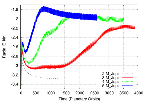
Figure 8: a) The time dependence of the total radial kinetic energy of the disk in the computational domain for four different planet masses. b) the growth rate of the eccentric disk mode as a function of the planetary mass. The superimposed straight line has a slope of $\tau\propto{M_{p}}^{-2.4}$.

3.5 Eccentricity growth rates

The growth of the eccentricity of the disk depends primarily on the mass of the planet. To measure the speed of the increase we analyze the time dependence of the total radial kinetic energy $E_{kin,rad}$ in the models, because this is a quantity most readily available. In the top panel of Fig. 8 we display the $E_{kin,rad}(t)$ for four different planet masses. For a low mass of $M_{p}=2M_{Jup}$ no growth is visible but for larger planets the growth time shortens upon increasing $M_{p}$. From the growth of $E_{kin,rad}(t)$ we estimate visually the growth-times $\tau$ as a function of planetary mass (lower panel of Fig. 8). Clearly, for more massive planets the disk will turn eccentric much faster. From the plot we may estimate a growth rate $\gamma=1/\tau\propto{M_{p}}^{2.4}$, a relation which is indicated by the additional straight line in the graph. This dependence on planetary mass is somewhat stronger than that estimated on theoretical grounds (Papaloizou et al. 2001).

Figure 9: The strength of several modes in the disk as a function of time. The solid line refers to the global disk eccentricity $S_{1,0}$. In the exponential growth regime the time derivative of the eccentricity (dotted line) is proportional to the (2,1) wave mode (short-dashed line).

3.6 Theoretical analysis

The observed growth of the disk eccentricity in our simulations resembles that found by Papaloizou et al. (2001) for very massive planets with $M_{p}\raisebox{-2.58334pt}{$\stackrel{{\scriptstyle{\displaystyle>}}}{{\sim}}$}10M_{Jup}$. The effect can be explained by a tidally driven eccentricity through resonant interaction of the disk with particular components of the planet’s gravitational potential (Lubow 1991a). Using cylindrical coordinates $(r,\varphi)$ we decompose the potential of the planet, which is on a circular orbit, in the form

$$\Phi_{p}(r,\varphi)=\sum_{m=0}^{m=\infty}\phi_{m}(r)\cos[m(\varphi-\Omega_{p}t)]$$ (3)

where $\Omega_{p}$ is the angular frequency of the planet. The response of the disk has the form

$$\propto\exp[i(k\varphi-l\Omega_{p}t)]$$

The planetary potential produces tides in the disk, which interact with an initially small eccentric disk. The $m$-th Fourier component of the potential (in Eq. 3) excites an eccentric Lindblad resonance in the outer disk where the rotation period of the disk is $\Omega={m\over{m+2}}\Omega_{P}$ which corresponds to the mode $(k,l)=(m+1,m)$ (Lubow 1991a). Hence, for an eccentric ($m=1$) perturbation the radial location lies at the outer 1:3 resonance at $r=2.08$. As the mass of the planetary companion increases, the gap it opens in the disk will be deeper and wider. Already in Artymowicz (1992) it was suggested that for sufficiently wide gaps, eccentricity growth can be induced by interaction at the 1:3 resonance in the outer disk, However, for smaller planet masses this is damped by other resonances which are listed in Goldreich & Sari (2003); Sari & Goldreich (2004). The main contributing eccentricity-damping resonances are the co-orbital resonances and the resonances located at the outer 1:2 resonance. Only if the gap is deep and wide enough these two resonances can no longer cancel the eccentricity-exciting effect of the interaction at the 1:3 resonance. The radial surface density profiles for simulations with different planet masses at 2500 orbits have been displayed in Fig. 3. As can be seen, only for planet masses larger than approximately 3 $M_{Jup}$ the gap is sufficiently cleared at the 1:2 resonance ($r\approx$ 1.58) to allow for an eccentricity increase of the disk.

Theoretical analysis in Lubow (1991b) defines the total mode strength $S_{k,l}$ as

$$S_{k,l}=(S^{2}_{cos,cos,k,l}+S^{2}_{cos,sin,k,l}+S^{2}_{sin,cos,k,l}+S^{2}_{sin,sin,k,l})^{1/2}$$

with $S_{f,g,k,l}$, defined in the inertial frame, given by

$$S_{f,g,k,l} = {2\over{\pi M(1+\delta_{i,0})(1+\delta_{j,0})}}\int\limits_{t}^{t+2\pi}dt^{\prime}\int dr\int\limits_{0}^{2\pi}rd\theta$$

$$\times\Sigma(r,\theta,t)f(i\theta)g(jt^{\prime})$$

In his analysis it is shown that the time derivative of the $k=1,l=0$ mode $S_{1,0}$ is given by the $k=2,l=1$ component:

$$\frac{S_{1,0}}{dt}\propto S_{2,1}\cdot S_{1,1}$$ (4)

The evolution of the relevant mode strengths for a model with $q=0.005$ is displayed in Fig. 9. The amplitude of the global eccentric mode ($k=1,l=0$) shows exponential growth (see Fig. 9, solid line). Furthermore, Eq. (4) is confirmed directly by comparing the $S_{2,1}$-mode (short-dashed line) and the numerically obtained derivative of the eccentricity, i.e. $S_{1,0}$ (dotted curve). As it can be seen from the plot, $S_{1,1}$ is constant as suggested by the theoretical analysis of Lubow (1991a).

The good agreement of our results with theoretical expectations supports our conclusion that the mechanism for eccentricity growth is that described by Lubow (1991a) and Papaloizou et al. (2001). In our simulations growth will start after the disk has settled sufficiently and the gap has been cleared, a process which occurs on viscous time scales. Our numerical growth rates during the eccentricity increase have been estimated from the time evolution of total radial kinetic energy (Fig. 8).

4 Conclusions

We have performed numerical time dependent hydrodynamical calculations of embedded planets in viscous accretion disks. During the evolution the planet is held fixed on a circular orbit, and the whole system is evolved in time until a quasi-equilibrium state has been reached. In contrast to previous existing simulations on this problem we have extended the evolutionary time to several thousand orbits of the embedded planet for a whole range of different planetary masses.

We find that beyond a certain critical mass of the planet the structure of the disk changes from a circular to an eccentric state. For typical viscosities in protoplanetary disks $\nu=10^{-5}$ (or $\alpha\approx 0.004$) the transition to the eccentric case occurs already for critical masses of $M_{p}=3M_{Jup}$. Through a modal analysis we demonstrate that the eccentric ($k=1,l=0$) mode in the disk is indeed driven by the ($k=2,l=1$) wave mode which is excited at the outer 1:3 Lindblad resonance. The numerically inferred growth rate of the unstable eccentric disk mode is roughly proportional to ${M_{p}}^{n}$ with $n=2.4$, which is slightly larger that the predicted value of $n=2.0$ (Lubow 1991a; Papaloizou et al. 2001). The discrepancy is most likely due to a change in the density structure of the gap for different planetary masses. For small masses $M_{p}=2M_{Jup}$ no eccentricity growth has been found. Here the damping effects of disk viscosity and pressure keep the disk in the circular state. Upon increasing the planetary mass the eccentricity eventually saturates at a value of $e\approx 0.25$.

The excitation of eccentric disk modes by massive companions has been studied within the framework of Cataclysmic Variable stars as an instability of the inner disk (Lubow 1991a, b). In those cases the change in viscous dissipation induced by the slow precession of the disk is presently the preferred mechanism to explain the observed superhumps in the light curve of some systems. That the same process is also applicable to (outer) disks around an embedded protoplanet has been confirmed by Papaloizou et al. (2001) in their study of very massive planets. In their simulations a much larger threshold mass ($\approx 10-20{\rm M_{\mathrm{Jup}}}$) has been found. However, their simulations were run only for 800 planetary orbits or less, which is not sufficient to see growth for small mass planets considering the long growth time of the eccentric mode.

The change in the state of the disk has significant consequences for the mass accretion rate onto the planet. For circular disks the width of the gap widens upon an increase in the planetary mass which shuts off eventually further accretion of disk material. The maximum mass a planet may reach by this process is around $5{\rm M_{\mathrm{Jup}}}$ (Bryden et al. 1999; Lubow et al. 1999). We suggest that through the excitation of the eccentric mode in the disk the planet can reach larger masses more readily, as there are quite a few systems with (minimum) planetary masses larger than $5M_{Jup}$. The influence an eccentric disk might have on the evolution of a pair of planets engaged in a 2:1 resonance has been analyzed recently by Kley et al. (2005). Here, changes in the libration amplitude of the resonant angles are to be expected.

It has been suggested that the gravitational back reaction of an embedded planet with the surrounding disk can lead to an increase in the orbital eccentricity of the planet (Goldreich & Sari 2003; Ogilvie & Lubow 2003), and may serve as a possible mechanism to explain the observed high eccentricities in extrasolar planetary systems. In the present work the gravitational back reaction of such an eccentric disk on the planetary orbit has not been analyzed, and remains to be studied in the future. The magnitude of the reachable eccentricity depends on the absolute physical mass of the ambient disk. Through numerical simulations Papaloizou et al. (2001) find that a significant increase in planetary eccentricity is only seen for a planet mass above $10\,M_{Jup}$. However, even in this case the maximum eccentricities do not increase beyond $e=0.25$. Additionally, the evolution time of the models was very short and did not allow to study the longterm evolution of the eccentricity.

As the effect of disk eccentricity scales with planet mass at least as $\propto{M_{p}}^{2.4}$ the effect is most pronounced for very massive planets. However, in that case it is also more difficult to induce high planetary eccentricities. Hence, it is very questionable if the back reaction of the disk can produce the observed high eccentricities found in the surveys.

The present study is only two dimensional and has not included any thermal effects such as radiative cooling or transport. Since in two dimensional calculations the gravitational effect between planet and disk tends to be over-estimated (as the disk is confined to the equatorial plane) one might expect a reduced effect in full three-dimensional simulations. But the very low value of the critical transition mass leaves sufficient room for an importance of this effect in the growth of extrasolar planets.