Local Ignition in Carbon/Oxygen White Dwarfs – I: One-zone Ignition and Spherical Shock Ignition of Detonations

Abstract

The details of ignition of Type Ia supernovae remain fuzzy, despite the importance of this input for any large-scale model of the final explosion. Here, we begin a process of understanding the ignition of these hotspots by examining the burning of one zone of material, and then investigate the ignition of a detonation due to rapid heating at single point.

We numerically measure the ignition delay time for onset of burning in mixtures of degenerate material and provide fitting formula for conditions of relevance in the Type Ia problem. Using the neon abundance as a proxy for the white dwarf progenitor’s metallicity, we then find that ignition times can decrease by $\sim 20\%$ with addition of even 5% of neon by mass. When temperature fluctuations that successfully kindle a region are very rare, such a reduction in ignition time can increase the probability of ignition by orders of magnitude. If the neon comes largely at the expense of carbon, a similar increase in the ignition time can occur.

We then consider the ignition of a detonation by an explosive energy input in one localized zone, e.g. a Sedov blast wave leading to a shock-ignited detonation. Building on previous work on curved detonations, we confirm that surprisingly large inputs of energy are required to successfully launch a detonation, leading to required matchheads of $\approx$ 4500 detonation thicknesses – tens of centimeters to hundreds of meters – which is orders of magnitude larger than naive considerations might suggest. This is a very difficult constraint to meet for some pictures of a deflagration-to-detonation transition, such as a Zel’dovich gradient mechanism ignition in the distributed burning regime.

1 INTRODUCTION

The current favored model for Type Ia supernovae (SNIa) involves burning beginning as a subsonic deflagration near the central region of a Chandrasekhar-mass white dwarf. Progress has been made in recent years in understanding the middle stages of these events through multiscale reactive flow simulations where the initial burning is prescribed as an initial condition of one or more sizable bubbles already burning material at time zero. However, the initial ignition process by which such bubbles begin burning – whether enormous 50 km bubbles (Plewa et al., 2004) or more physically motivated smaller igniting points (Reinecke et al., 2002; Höflich and Stein, 2002; Bravo and García-Senz, 2003) remains poorly understood. Further, if later in the evolution there is a transition to a detonation (e.g., Gamezo et al., 2004), this ignition process, too, must be explained. Indeed, ignition physics will play a role — by determining the location, number, and sizes of the first burning points — in any currently viable SNIa model. However, until very recently (for example, Woosley et al., 2004; García-Senz and Bravo, 2005) very little work has gone into examining the ignition physics of these events. Here we begin examining the ignition process by considering the simplest ignitions possible – that of a single zone – and the possibility of igniting a detonation from a Sedov blast wave launched at a single point.

1.1 Ignition Delay Times

Astrophysical combustion, like most combustion (for example, Williams, 1985; Glassman, 1996), is highly temperature-dependent; the ¹²C + ¹²C reaction, for example, scales as $T^{12}$ near 10⁹ K. Rates for the exothermic reactions which define the burning process are generally exponential or near-exponential in temperature (e.g., Caughlan and Fowler, 1988). Thus a region with a positive temperature perturbation can sit ‘simmering’ for a very long time, initially only very slowly consuming fuel and increasing its temperature as an exponential runaway occurs. This is especially true in the electron-degenerate environment of a white dwarf, where the small increases in temperature that occur for most of the evolution of the hotspot will have only extremely small hydrodynamic effects.

If fuel depletion and hydrodynamical effects were ignored, the temperature of the spot would become infinite after a finite period of time. This time is called the ignition time, or ignition delay time, or sometimes induction time, $\tau_{i}$. After ignition starts, burning proceeds for some length of time $\tau_{b}$.

For burning problems of interest, of course, fuel depletion is important, and no quantities become infinite; however, the idea of an ignition delay time still holds (see Fig. 1). If the energy release rate for most of the evolution of the burning is too small to have significant hydrodynamical effects, and if the timescale over which burning ‘suddenly turns on’ is much shorter than any other hydrodynamical or conductive timescales, then the burning of such a hotspot can be treated, as an excellent approximation, as a step function where all energy is released from $t=\tau_{i}$ to $t=\tau_{i}+\tau_{b}$. In many problems, where $\tau_{b}\ll\tau_{i}$, this can be further simplified to burning occurring only at $t=\tau_{i}$. Where such an approximation (often called ‘high activation-energy asymptotics’) holds, it greatly simplifies many problems of burning or ignition, reducing the region of burning in a flame to an infinitesimally thin ‘flamelet’ (Matalon and Matkowsky, 1982) surface, for instance, or the structure of a detonation to a ‘square wave’ (Erpenbeck, 1963). Where this approximation does not hold – such as if slow $\beta$-decay processes are important as bottlenecks for reactions to proceed (e.g., $p$-$p$ burning or the CNO cycle) the simplification of burning happening only over $\tau_{i}\leq t\leq\tau_{i}+\tau_{b}$ often remains useful.

Even for the simple case of one zone, ignition delay times are relevant for investigation of ignition in SNIa because it sets a minimum time scale over which an initial local positive temperature perturbation (hot spot) can successfully ignite and launch a combustion wave; other timescales, such as turbulent disruption of the hotspot, or diffusive timescales, must be larger than this for ignition to successfully occur.

Figure 1: Temperature evolution for burning a zone at constant pressure with an initial state of $X_{\mathrm{{}^{12}{C}}}=1.0$, $T=10^{9}\mathrm{K}$, $\rho=5\times 10^{8}\mathrm{g\ cm^{-3}}$. Because of the strong temperature dependence, a runaway takes place and most of the burning happens ‘all at once’.

If the burning occurs in an ideal gas, or in a material with some other simple equation of state, it is fairly easy to write down approximate ignition times for various burning laws. In a white dwarf, however, where the material is partially degenerate or relativistic and the equation of state is quite complicated (Timmes and Swesty, 2000), no such closed-form expression can be written. In §2 we numerically follow the abundance and thermodynamic evolution of a zone of white dwarf material in order to measure the ignition times as a function of the initial temperature, density, and composition. We follow both constant-density and constant-pressure trajectories. The results are summarized by simple, moderately accurate, fitting formula. In §3 we consider the ignition of a detonation through a localized energy release producing a Sedov blast wave, and estimate the amount of energy that must be released for the detonation to successfully ignite. In §4 we consider our results in light of likely temperature fluctuation spectra during the simmering, convective phase.

2 ONE ZONE IGNITION TIMES

2.1 Calculations

We performed a series of 1-zone calculations for the purposes of measuring ignition times in carbon-oxygen mixtures. For each of these two burning conditions – burning at constant volume and constant pressure – over 3500 initial conditions were examined, in a grid of initial densities, temperatures, and initial carbon fraction. The carbon (mass) fractions were in the range $0.4\leq X_{\mathrm{{}^{12}{C}}}\leq 1.0$, with the remainder being oxygen ($X_{\mathrm{{}^{16}{O}}}=1-X_{\mathrm{{}^{12}{C}}}$), temperatures of $0.5\leq T_{9}\leq 7$, and densities $0.1\leq\rho_{8}\leq 50$, where $T_{9}$ is the temperature in units of $10^{9}$ K and $\rho_{8}$ is the density in units of $10^{8}$ g cm^-3. For burning, a 13-isotope $\alpha$ chain was used (Timmes, 1999), and a Helmholtz free energy based stellar equation of state (Timmes and Swesty, 2000) maintained the thermodynamic state. The temperature and abundance evolution equations were integrated together consistently, as described in Appendix A. Time evolutions were generated as in Fig. 1.

To cover the wide range of burning times within each integration, the timestep was increased or decreased depending on the rate of abundance, energy release, and thermodynamic changes. The time interval was varied by up to a factor of two in each timestep, to try to keep the amount of energy released through burning per timestep change of fuel within the range $10^{-5}-10^{-7}$. Timesteps failing this criterion were undone and re-taken with a smaller time interval. The final ignition time, when the simulation was stopped, was defined to be time when 90% of the carbon was consumed, although the time reported was found to be insensitive to endpoint chosen. The code used in this integration, as well as the resulting data, is available at http://www.cita.utoronto.ca/$∼$ljdursi/ignition/.

Over the initial conditions chosen, ignition times varied from $10^{-14}$ s to $10^{+8}$ s. A representative contour plot showing the calculated ignition delay times are shown in Fig. 2.

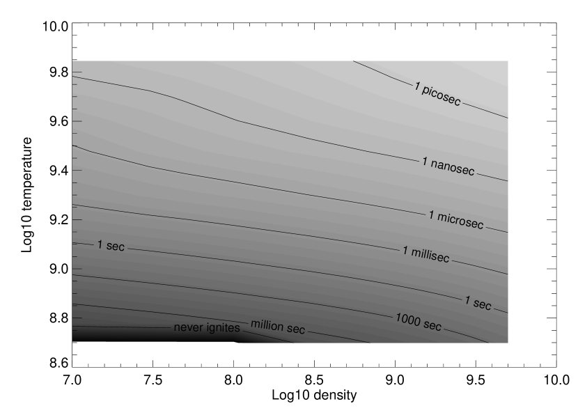
Figure 2: Contour plot of ignition time as a function of initial density and temperature for a constant-pressure ignition of a mixture of half-carbon, half-oxygen by mass.

Fitting formula for the ignition delay times under the two burning conditions were determined; the ignition time for constant-pressure ignition can be given approximately as

$$\tau_{i,{\mathrm{cp}}}(\rho,T,X_{\mathrm{{}^{12}{C}}}) = 1.15\times 10^{-5}\,\mathrm{sec}\,\left(X_{\mathrm{{}^{12}{C}}}\rho_{8}\right)^{-1.9}f_{\mathrm{cp}}(T)\left(1+1193f_{\mathrm{cp}}(T)\right)$$ (1)

$$f_{\mathrm{cp}}(T) = \left(T_{9}-0.214\right)^{-7.566}$$

and that for constant-volume ignition

$$\tau_{i,{\mathrm{cv}}}(\rho,T,X_{\mathrm{{}^{12}{C}}}) = 1.81\times 10^{-5}\,\mathrm{sec}\,\left(X_{\mathrm{{}^{12}{C}}}\rho_{8}\right)^{-1.85}f_{\mathrm{cv}}(T)\left(1+1178f_{\mathrm{cv}}(T)\right)$$ (2)

$$f_{\mathrm{cv}}(T) = \left(T_{9}-0.206\right)^{-7.700}$$

where $T_{9}$ is the initial temperature in units of $10^{9}\mathrm{K}$, and $\rho_{8}$ is the initial density in units of $10^{8}\mathrm{g\ cm^{-3}}$.

The fits are good to within a factor of five between $10^{-9}$ sec and $1$ sec, and to within a factor of 10 between $10^{-14}$ sec and $100$ sec. This can be compared to other analytic expressions, for instance the constant-pressure formula from Woosley et al. (2004),

$${\tau_{i}}=15~{}{\mathrm{sec}}\left(\frac{7}{T_{8}}\right)^{22}\left(\frac{2}{\rho_{9}}\right)^{3.3}$$ (3)

which, as shown in Fig. 4, is an excellent approximation over a somewhat more narrow range of conditions.

Figure 3: Fit results vs. calculated results for constant-pressure (left) and constant-volume (right) ignition delay times, for the full range of densities ($0.1\leq\rho_{8}\leq 50$), temperatures ($0.5\leq T_{9}\leq 7$), and carbon mass abundances ($0.4\leq X_{\mathrm{{}^{12}{C}}}\leq 1.0$) considered.

Figure 4: Woosley et al. (2004) ignition time results vs. calculated results for constant-pressure ignition delay times for a mixture half-carbon half-oxygen by mass ($X_{\mathrm{{}^{12}{C}}}=0.5$), over a truncated range ($1\leq\rho_{8}\leq 50$), ($0.5\leq T_{9}\leq 1.5$).

Which of the two cases (constant volume or constant pressure) are appropriate will depend on comparing the ignition time with the relevant hydrodynamical timescale — in particular, the sound-crossing time of the region undergoing ignition. If the region is small enough that many sound crossing times occur during the ignition, then the constant-pressure value is appropriate; if ignition occurs in much less than a crossing time, the constant-volume value is appropriate; intermediate timescales will result in intermediate values. In the case of turbulent ignition of a flame, presumably it is the constant-pressure time which will be most relevant. In any case, due to the degeneracy of the material in the density and temperature ranges considered here, the computed ignition times (or the fits) rarely differ between the two cases more than 50%.

2.2 Effect of Metallicity

Most of the initial metallicity of main-sequence star comes from the CNO and $\mathrm{{}^{56}{Fe}}$ nuclei inherited from its ambient interstellar medium at birth. The slowest step in the hydrogen-burning CNO cycle is proton capture onto $\mathrm{{}^{14}{N}}$. This results in all the CNO catalysts piling up into $\mathrm{{}^{14}{N}}$ when hydrogen burning on the main sequence is completed. During helium burning, all of the $\mathrm{{}^{14}{N}}$ is converted into $\mathrm{{}^{22}{Ne}}$.

As a proxy for investigating the effects of metallicity in our $\alpha$-chain based reaction network, we consider the ignition of a $X_{\mathrm{{}^{12}{C}}}=0.5$ constant-pressure ignition while increasing the fraction of $\mathrm{{}^{20}{Ne}}$ (and thus decreasing the abundance of oxygen). We’ll verify this surrogate by using $\mathrm{{}^{22}{Ne}}$ in larger networks.

The effects of increasing $X_{\mathrm{{}^{20}{Ne}}}$ from 0 to 0.05, and then further to 0.1 and 0.2, is shown in Fig. 5. Addition of even fairly modest amounts of neon can significantly (20–30%) reduce the ignition times for much of the thermodynamic conditions evaluated here. The reduced ignition times are found to result from a larger energy release from burning over the entire integration range.

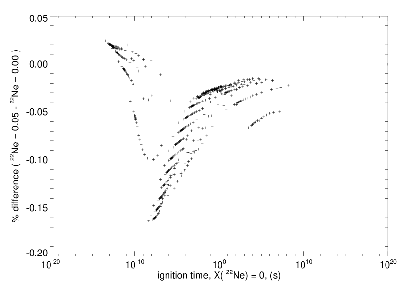
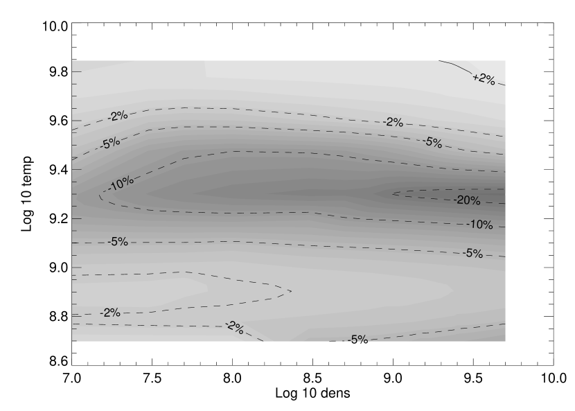
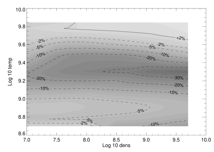
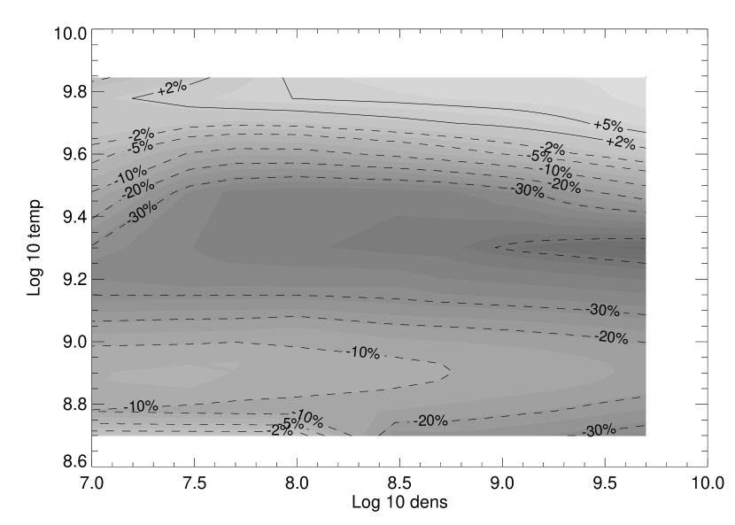
Figure 5: The difference in ignition time for a constant-pressure ignition of $X_{\mathrm{{}^{12}{C}}}=0.5$, $X_{\mathrm{{}^{16}{O}}}=0.5$ when some of the Oxygen is replaced by Neon-20. On the top left is shown the fractional difference in ignition time with the addition of $X_{\mathrm{{}^{20}{Ne}}}=0.05$ as a function of the ignition time with $X_{\mathrm{{}^{20}{Ne}}}=0.0$. On the top right, bottom left, and bottom right are contour plots in $\rho-T$ space of the percent difference in ignition time with $X_{\mathrm{{}^{20}{Ne}}}=0.05,0.1,0.2$, respectively. The ignition time for the base case is shown in Fig. 2.

To understand the increase in the energy deposited by burning, consider the $\alpha$-chain reactions which dominate burning in this regime and are modeled by the ‘aprox13’ network as:

$$\mathrm{{}^{12}{C}}+\mathrm{{}^{12}{C}} \rightarrow \mathrm{{}^{20}{Ne}}+\alpha+13.933\,\mathrm{MeV}$$

$$\mathrm{{}^{12}{C}}+\alpha \rightarrow \mathrm{{}^{16}{O}}+7.162\,\mathrm{MeV}$$

$$\mathrm{{}^{16}{O}}+\alpha \rightarrow \mathrm{{}^{20}{Ne}}+4.734\,\mathrm{MeV}$$ (4)

$$\mathrm{{}^{20}{Ne}}+\alpha \rightarrow \mathrm{{}^{24}{Mg}}+9.312\,\mathrm{MeV}$$

$$\mathrm{{}^{24}{Mg}}+\alpha \rightarrow \mathrm{{}^{28}{Si}}+9.984\,\mathrm{MeV}.$$

Given an initial mixture of $\mathrm{{}^{12}{C}}$, $\mathrm{{}^{16}{O}}$, and $\mathrm{{}^{20}{Ne}}$, it is the carbon burning reaction $\mathrm{{}^{12}{C}}+\mathrm{{}^{12}{C}}$ which happens first. The resulting $\alpha$-particle can capture onto carbon or any heavier element in the $\alpha$ chain. Unless that chain is already populated, then the (very exothermic) neon capture and all flows to still heavier nuclei are choked off until enough $\mathrm{{}^{20}{Ne}}$ and $\mathrm{{}^{24}{Mg}}$ are generated through burning. Adding even quite modest amounts of neon to the initial mixture allows more $\alpha$-chain reactions to promptly occur during carbon burning.

The plots in Fig. 6 show the abundance evolution of $\alpha$-chain elements during constant-density burning at $\rho_{8}=10$, $T_{9}=1$, $X_{\mathrm{{}^{12}{C}}}=0.5$, and an initial neon abundance of zero and 0.05. The inclusion of 5% neon by mass greatly speeds the production of heavier intermediate-mass elements, and thus the exothermicity of the burning, reducing the ignition time.

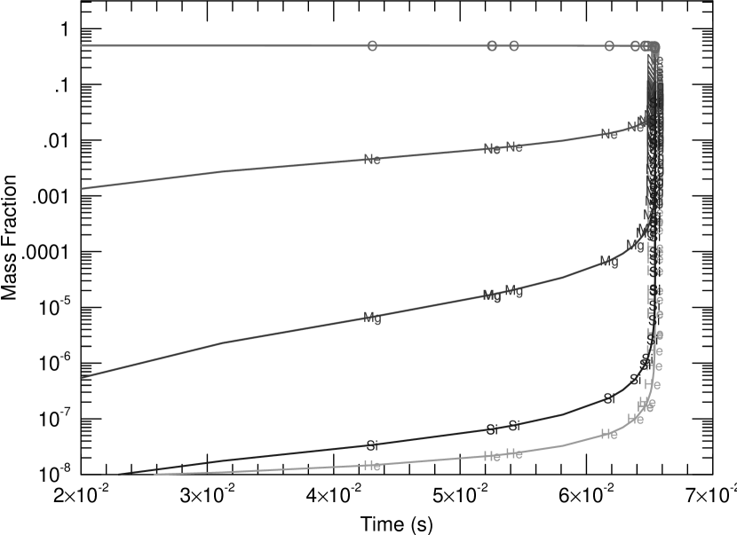
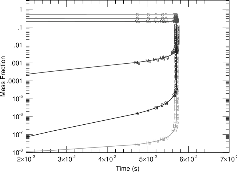
Figure 6: Mass fraction evolution in constant-density burning, with an initial state of $\rho_{8}=10$, $T_{9}=1$, $X_{\mathrm{{}^{12}{C}}}=0.5$, with $X_{\mathrm{{}^{20}{Ne}}}=0.0$ (left) and $X_{\mathrm{{}^{20}{Ne}}}=0.1$ (right). The burning here was calculated with a 513-isotope network. Because of the removal of the $\alpha$-chain bottleneck at neon on the right, burning proceeds faster and the generation of higher intermediate-mass elements is raised by orders of magnitude at early times.

To confirm that this effect is not artificially enhanced by using an $\alpha$-chain reaction network, and to quantitatively verify the ignition times produced by the aprox13 network used here, we compared the ignition times at two $(\rho,T)$ points and varying neon abundance with those produced by reaction networks containing 513 and 3304 isotopes. The results are shown in Table 1 We see that not only are the times computed with the smaller network quantitatively in good agreement with the larger networks (within 10% for the lower-temperature case, and within 25% for the higher case), but the trends are similar. The same trend is apparent when $\mathrm{{}^{22}{Ne}}$, unavailable in the $\alpha$-chain network, is used instead of $\mathrm{{}^{20}{Ne}}$. The trend is in fact stronger with $\mathrm{{}^{22}{Ne}}$ because of additional flow paths that become available.

Table 1: Constant-volume ignition times (sec) adding Neon with different reaction networks

				$\rho_{8}=10,T_{9}=1$			$\rho_{8}=1,T_{9}=3$
$X_{\mathrm{{}^{12}{C}}}$	$X_{\mathrm{{}^{16}{O}}}$	$X_{\mathrm{{}^{20}{Ne}}}$	$X_{\mathrm{{}^{22}{Ne}}}$	13 isotopes	513 isotopes	3304 isotopes	13 isotopes	513 isotopes
$0.5$	$0.5$	$0.0$	$0.0$	$5.96\times 10^{-2}$	$6.42\times 10^{-2}$	$6.42\times 10^{-2}$	$2.16\times 10^{-8}$	$1.74\times 10^{-8}$
$0.5$	$0.45$	$0.05$	$0.0$	$5.77\times 10^{-2}$	$6.49\times 10^{-2}$		$1.94\times 10^{-8}$	$1.58\times 10^{-8}$
$0.5$	$0.4$	$0.1$	$0.0$	$5.58\times 10^{-2}$	$6.38\times 10^{-2}$	$6.38\times 10^{-2}$	$1.79\times 10^{-8}$	$1.49\times 10^{-8}$
$0.5$	$0.3$	$0.2$	$0.0$	$5.18\times 10^{-2}$	$6.09\times 10^{-2}$		$1.60\times 10^{-8}$	$1.37\times 10^{-8}$
$0.5$	$0.45$	$0.0$	$0.05$		$5.56\times 10^{-2}$			$9.61\times 10^{-9}$
$0.5$	$0.4$	$0.0$	$0.1$		$5.54\times 10^{-2}$	$5.54\times 10^{-2}$		$9.04\times 10^{-9}$
$0.5$	$0.3$	$0.0$	$0.2$		$5.64\times 10^{-2}$			$8.92\times 10^{-9}$

While the above has demonstrated the active role neon plays in the ignition process, its effect is much smaller than that of carbon, which is the primary source of fuel in this burning process. As a result, in the more realistic case when an increase in neon comes at the expense of both carbon and oxygen, this effect is reduced (for small neon fractions) or completely reversed (for moderate neon fractions). This is shown, for instance, in Fig. 7. In this case, increased metallicity of the progenitor system has the opposite effect; it makes the ignition time significantly longer for hotspots in the resulting white dwarf.

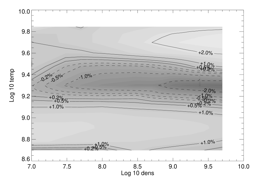
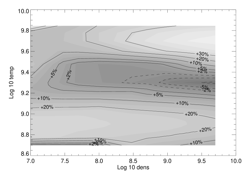
Figure 7: As in Fig. 5, the difference in ignition time for a constant-pressure ignition of $X_{\mathrm{{}^{12}{C}}}=0.5$, $X_{\mathrm{{}^{16}{O}}}=0.5$ when (left) a mass fraction of 0.005 of each of the carbon and oxygen is replaced by Neon-20 and (right) when 0.05 of each is replaced by Neon. Note that in this case, for $X_{\mathrm{{}^{20}{Ne}}}=0.1$, with the exception of a small region in ($\rho$,$T$) the ignition time is increased by the same magnitude that it is decreased in the case when all of the neon comes from oxygen, e.g. the $X_{\mathrm{{}^{12}{C}}}=0.5$,$X_{\mathrm{{}^{16}{O}}}=0.4$,$X_{\mathrm{{}^{20}{Ne}}}=0.1$ case of Fig 5 in the bottom right panel.

3 APPLICATION: IGNITION OF A DETONATION

3.1 Detonation Structure

Detonation waves are a supersonic mode of propagating combustion. A shock wave heats up material, which then ignites, releasing energy which further powers the shock. (See, for instance, textbooks such as Glassman, 1996; Williams, 1985). There are, broadly, four states in a detonation: the unshocked material; the shocked material immediately behind the shock; an induction zone, where the heated material slowly begins burning and then the reaction zone, where the bulk of the exothermic burning takes place.

Unsupported, self-sustaining detonations can be of the Chapman-Jouget (CJ) type, where at the end of the reaction zone the flow becomes sonic, or of the pathological type, where the sonic point occurs within reaction zone, decoupling the flow downstream of the sonic point from the shock. Pathological detonations can occur in material where there are endothermic reactions or other dissipative or cooling effects, and may have speeds slightly higher (typically by a few percent) than the CJ speed. Detonations within highly degenerate white-dwarf material ($\rho_{8}>0.2$) are of the pathological type (Khokhlov, 1989), largely because some regions of the flow behind the detonation can have significant amounts of endothermic reactions, violating the assumptions of the CJ structure. Because in the case of a pathological detonation some fraction of the reactions powering the detonation are decoupled from the shock, calculating the speed of a pathological detonation requires detailed integration of the detonation structure, rather than simply using jump conditions. For either kind of detonation, one can estimate where most burning occurs with shock speed $D$ (which, even in non-CJ case, can be estimated with CJ speed) and $\tau_{i}$; $l_{i}=D\tau_{i}$ is the position behind the shock at which the induction zone ends and rapid burning takes place.

In the case of a detonation into a very low-density, cold material, the material immediately behind the shock will still not burn significantly until a length of time equal to the ignition time passes, resulting in a ‘square wave’ detonation. For conditions relevant to near the core of a white dwarf, however, the post-shock fluid will typically have temperatures on order $T_{9}\approx 5$ – that is, temperatures which are already near the maximum temperature which will be obtained by burning. Even in these cases, this estimate of $l_{i}$ provides a good measure of the thickness of the detonation structure behind the shock, as is shown in Fig 8 where it measures the position of maximum burning.

Figure 8: Two examples of estimating the detonation thickness, $l_{i}=v_{s}\tau_{i}$ in a detonation. On the left, plotted energy release rate from nuclear reactions behind the shock of a leftward-traveling ZND detonation into a pure-carbon quiescent medium of $\rho_{8}=1$, $T_{9}=0.05$. The shocked state is $\rho_{8}=2.97$, $T_{9}=4.2$, and the incoming fuel velocity behind the shock is $4.0\times 10^{8}\mathrm{cm\ s^{-1}}$. For the shocked material, the predicted ignition time is $\approx 3\times 10^{-11}\mathrm{sec}$. Even in this case, where the shocked temperature is so high that significant burning occurs immediately, and the ‘square wave’ detonation structure does not apply, the predicted $l_{i}=1.2\times 10^{-2}\mathrm{cm}$ correctly matches the peak of the reaction zone. On the right, pressure (top) and energy release rate (bottom), plotted relative to their maximum values, behind a leftward-traveling slightly overdriven detonation into the same material as in the previous figure, calculated by the hydrodynamics code Flash (Fryxell et al., 2000; Calder et al., 2002). The line above the plotted quantities shows the predicted $l_{i}$ calculated with the observed values in the shocked state.

3.2 Ignition of a Spherical Detonation

One mechanism for ignition of a detonation by a hotspot is an initial rapid input of energy which leads to a Sedov blast wave; the material shocked by the outgoing spherical blast ignites, and as the outgoing wave slows, a steady outgoing detonation results. A steady detonation cannot form until the outgoing shock wave speed drops to the detonation velocity detonation, or else the energy released by reactions behind the blast wave will not be able to ‘catch up’ to the outgoing shock to drive it. On the other hand, if the shock drops significantly below the detonation speed before ignition takes place, not enough material will be burning per unit time to sustain a detonation wave. We denote the position of the shock when it reaches the detonation speed from above as $R_{D}$. Naively, the condition for successful detonation ignition would be that $R_{D}\gtrsim l_{i}$, since a detonation structure with width of order $l_{i}$ must be set up before the shock speed becomes too slow; a more sophisticated derivation of this criterion can be found in Zeldovich et al. (1956). However, experimentally this is known to be far too lenient a condition for terrestrial detonations and $R_{D}$ must be orders of magnitude larger than $l_{i}$ (Desbordes, 1986). This has also been empirically seen in the context of astrophysical detonations (e.g., Niemeyer and Woosley, 1997).

This has been explained by, for instance, He and Clavin (1994). Curvature has a significant nonlinear effect on the structure of a detonation — even more so than on the structure of a flame (e.g., Dursi et al., 2003) because the curvature directly effects the burning region rather than merely the preconditioning (diffusion) region. He and Clavin (1994), looking at a pseudo-steady calculation of a detonation with curvature, find that for a steady detonation to exist requires the curvature to be extremely small. The condition found by the authors requires $R_{D}\approx 44\gamma^{2}/(\gamma^{2}-1)\beta_{Z}l_{i}$, where $\gamma$ is the polytropic index of the ideal gas and $\beta_{Z}$ represents the temperature sensitivity of the burning law; for the reactions and temperatures of interest in astrophysical combustion, $\beta_{Z}\approx 10-15$ (Dursi et al., 2003). Using $\gamma=4/3$ to describe the highly degenerate material near the centre of the white dwarf, this would give $R_{D}\approx 1000-1500l_{i}$.

While in many cases using a polytropic ideal gas equation of state to describe degenerate white dwarf material can be an excellent approximation, in combustion phenomenon where the burning rate is highly temperature dependent it is problematic, making the above result unsuitable. Further, the authors assume a CJ detonation, as opposed to the pathological detonation that occurs at high densities in a white dwarf. This makes a straightforward application of the results of He and Clavin (1994) to our problem of interest difficult. Given the complexity of the partially degenerate equation of state in the white dwarf, re-deriving the analytic results for this application would be difficult. However, the detailed effect of curvature on detonations in white dwarfs has already been studied in a different manner, by Sharpe (2001). In this approach, the velocity eigenvalue for the detonation – which depends sensitively on the detonation structure – is calculated using a shooting method to numerically integrate the structure of a pathological detonation to the sonic point. A range of possible detonation velocities is input, and then repeatedly bisected as the detonation structure with a fixed given curvature term is integrated assuming the current detonation velocity. The result is the velocity-curvature relation for a detonation into a given ambient material, and as a byproduct, the relationship between the thermodynamic structure (at least up to the sonic point) and the curvature for the curved detonation.

We follow the method of Sharpe (2001), also described in Appendix B, and measure the maximum sustainable spherical curvature of a detonation using the same equation of state and burning network as used in the ignition time study. An example of the detonation-speed versus curvature relation is given in Fig. 9. Beyond some maximum curvature $\kappa_{\mathrm{max}}$, no steady-state unsupported detonation can exist; thus in the case of a spherical detonation, for a steady detonation to successfully ignite, $R_{D}>\kappa_{\mathrm{max}}^{-1}$.

Figure 9: Example of detonation speed vs. curvature, for a detonation into a quiescent medium of $\rho_{8}=1$, $T_{9}=0.05$, $X_{\mathrm{{}^{12}{C}}}=0.5$, $X_{\mathrm{{}^{16}{O}}}=0.5$.

We calculated the detonation speed versus curvature relation for $0.5\leq\rho_{8}\leq 20$ and $0.25\leq X_{\mathrm{{}^{12}{C}}}\leq 1.0$. The unshocked material was set to a temperature of $T_{9}=0.05$, although the results were seen to be insensitive to this value. Our results are shown in Fig. 10 and Table 2. The code used to perform the calculations is available at http://www.cita.utoronto.ca/$∼$ljdursi/ignition. The estimated detonation thickness and a comparison with $\kappa_{\mathrm{max}}$ is given in Table 3. As compared with the He and Clavin (1994) results of $R_{D}\gtrsim 1000-1500l_{i}$, we find $R_{D}\gtrsim 3000-6000l_{i}$.

Figure 10: Steady-state detonation velocity as a function of curvature for background densities of, from left to right and top to bottom, $\rho_{8}=(0.5,1,2,5,10,20)$. In each plot, the velocities are shown for initial carbon abundances, top to bottom, of $X_{\mathrm{{}^{12}{C}}}=(1,0.75,0.5,0.25)$. So that they could be shown on the same horizontal scale, the curvatures have been scaled to the maximum sustainable curvature for each set of conditions, given by Table 2. Points represent calculated speeds, and solid lines are fits with parameters also given in Table 2.

Table 2: Measured and Fit Detonation Velocities as a function of curvature

	$D$	$\kappa_{\mathrm{max}}$	$v_{\mathrm{max}}$	Fit Parameters
	$(10^{9}\mathrm{cm})$	$\mathrm{cm}^{-1}$	$10^{9}\mathrm{cm}$	$a$	$b$	$c$	$d$
$\rho_{8}=0.5$
$X_{\mathrm{{}^{12}{C}}}=1.00$	$1.207$	$1.08\times 10^{-2}$	$1.096$	$-1.55\times 10^{-2}$	$7.75\times 10^{-1}$	$-1.26\times 10^{0}$	$1.51\times 10^{0}$
$X_{\mathrm{{}^{12}{C}}}=0.75$	$1.181$	$2.94\times 10^{-3}$	$1.069$	$-5.74\times 10^{-4}$	$4.68\times 10^{-1}$	$4.07\times 10^{-1}$	$1.26\times 10^{-1}$
$X_{\mathrm{{}^{12}{C}}}=0.50$	$1.152$	$7.14\times 10^{-4}$	$1.067$	$-1.78\times 10^{-3}$	$6.11\times 10^{-1}$	$7.21\times 10^{-1}$	$-3.30\times 10^{-1}$
$X_{\mathrm{{}^{12}{C}}}=0.25$	$1.120$	$1.26\times 10^{-4}$	$1.055$	$-2.27\times 10^{-3}$	$1.15\times 10^{0}$	$-1.39\times 10^{-1}$	$-7.54\times 10^{-3}$
$X_{\mathrm{{}^{12}{C}}}=0.125$	$1.110$	$2.34\times 10^{-5}$	$1.059$	$-1.32\times 10^{-2}$	$1.20\times 10^{0}$	$-1.65\times 10^{-0}$	$1.37\times 10^{-3}$
$\rho_{8}=1.$
$X_{\mathrm{{}^{12}{C}}}=1.00$	$1.218$	$2.78\times 10^{-2}$	$1.131$	$-4.69\times 10^{-3}$	$6.25\times 10^{-1}$	$1.87\times 10^{-3}$	$3.77\times 10^{-1}$
$X_{\mathrm{{}^{12}{C}}}=0.75$	$1.195$	$1.02\times 10^{-2}$	$1.116$	$-4.08\times 10^{-3}$	$6.53\times 10^{-1}$	$3.30\times 10^{-1}$	$2.06\times 10^{-2}$
$X_{\mathrm{{}^{12}{C}}}=0.50$	$1.170$	$3.15\times 10^{-3}$	$1.102$	$-5.41\times 10^{-3}$	$8.30\times 10^{-1}$	$2.64\times 10^{-1}$	$-8.85\times 10^{-2}$
$X_{\mathrm{{}^{12}{C}}}=0.25$	$1.141$	$5.58\times 10^{-4}$	$1.085$	$-2.99\times 10^{-3}$	$1.17\times 10^{0}$	$-2.12\times 10^{-1}$	$4.44\times 10^{-2}$
$X_{\mathrm{{}^{12}{C}}}=0.125$	$1.126$	$8.90\times 10^{-5}$	$1.092$	$-9.94\times 10^{-3}$	$9.55\times 10^{-1}$	$1.35\times 10^{-1}$	$-7.99\times 10^{-2}$
$\rho_{8}=2.$
$X_{\mathrm{{}^{12}{C}}}=1.00$	$1.249$	$6.67\times 10^{-2}$	$1.176$	$-5.52\times 10^{-4}$	$7.93\times 10^{-1}$	$8.76\times 10^{-2}$	$1.20\times 10^{-1}$
$X_{\mathrm{{}^{12}{C}}}=0.75$	$1.227$	$2.72\times 10^{-2}$	$1.169$	$-2.72\times 10^{-3}$	$6.75\times 10^{-1}$	$4.44\times 10^{-1}$	$-1.16\times 10^{-1}$
$X_{\mathrm{{}^{12}{C}}}=0.50$	$1.203$	$8.90\times 10^{-3}$	$1.152$	$-1.07\times 10^{-2}$	$9.50\times 10^{-1}$	$1.07\times 10^{-1}$	$-4.54\times 10^{-2}$
$X_{\mathrm{{}^{12}{C}}}=0.25$	$1.177$	$1.56\times 10^{-3}$	$1.133$	$-8.23\times 10^{-3}$	$1.10\times 10^{0}$	$-9.81\times 10^{-2}$	$2.26\times 10^{-3}$
$X_{\mathrm{{}^{12}{C}}}=0.125$	$1.163$	$2.71\times 10^{-4}$	$1.127$	$-1.07\times 10^{-3}$	$1.18\times 10^{0}$	$-2.05\times 10^{-1}$	$3.07\times 10^{-2}$
$\rho_{8}=5.$
$X_{\mathrm{{}^{12}{C}}}=1.00$	$1.316$	$1.96\times 10^{-1}$	$1.257$	$-5.81\times 10^{-3}$	$8.76\times 10^{-1}$	$1.20\times 10^{-1}$	$9.98\times 10^{-3}$
$X_{\mathrm{{}^{12}{C}}}=0.75$	$1.295$	$8.49\times 10^{-2}$	$1.241$	$1.24\times 10^{-3}$	$1.11\times 10^{0}$	$-2.25\times 10^{-1}$	$1.11\times 10^{-1}$
$X_{\mathrm{{}^{12}{C}}}=0.50$	$1.273$	$2.76\times 10^{-2}$	$1.227$	$-3.67\times 10^{-3}$	$1.16\times 10^{0}$	$-2.27\times 10^{-1}$	$6.94\times 10^{-2}$
$X_{\mathrm{{}^{12}{C}}}=0.25$	$1.248$	$4.75\times 10^{-3}$	$1.210$	$-8.00\times 10^{-3}$	$1.19\times 10^{0}$	$-2.25\times 10^{-1}$	$4.18\times 10^{-2}$
$X_{\mathrm{{}^{12}{C}}}=0.125$	$1.235$	$9.30\times 10^{-4}$	$1.205$	$-9.26\times 10^{-3}$	$8.82\times 10^{-1}$	$2.83\times 10^{-1}$	$-1.56\times 10^{-1}$
$\rho_{8}=10.$
$X_{\mathrm{{}^{12}{C}}}=1.00$	$1.386$	$4.45\times 10^{-1}$	$1.327$	$-1.31\times 10^{-4}$	$1.04\times 10^{0}$	$-1.53\times 10^{-1}$	$1.10\times 10^{-1}$
$X_{\mathrm{{}^{12}{C}}}=0.75$	$1.366$	$1.94\times 10^{-1}$	$1.316$	$-2.65\times 10^{-3}$	$1.08\times 10^{0}$	$-1.19\times 10^{-1}$	$4.04\times 10^{-2}$
$X_{\mathrm{{}^{12}{C}}}=0.50$	$1.343$	$6.27\times 10^{-2}$	$1.298$	$6.40\times 10^{-3}$	$1.26\times 10^{0}$	$-3.40\times 10^{-1}$	$7.62\times 10^{-2}$
$X_{\mathrm{{}^{12}{C}}}=0.25$	$1.319$	$1.06\times 10^{-2}$	$1.279$	$6.21\times 10^{-4}$	$1.40\times 10^{0}$	$-5.84\times 10^{-1}$	$1.81\times 10^{-1}$
$X_{\mathrm{{}^{12}{C}}}=0.125$	$1.306$	$2.24\times 10^{-3}$	$1.269$	$-5.93\times 10^{-3}$	$1.35\times 10^{0}$	$-4.74\times 10^{-1}$	$1.26\times 10^{-1}$
$\rho_{8}=20.$
$X_{\mathrm{{}^{12}{C}}}=1.00$	$1.472$	$1.03\times 10^{0}$	$1.411$	$1.03\times 10^{-5}$	$1.14\times 10^{0}$	$-2.99\times 10^{-1}$	$1.59\times 10^{-1}$
$X_{\mathrm{{}^{12}{C}}}=0.75$	$1.451$	$4.56\times 10^{-1}$	$1.399$	$-1.93\times 10^{-3}$	$1.26\times 10^{0}$	$-4.25\times 10^{-1}$	$1.68\times 10^{-1}$
$X_{\mathrm{{}^{12}{C}}}=0.50$	$1.429$	$1.47\times 10^{-1}$	$1.382$	$2.49\times 10^{-4}$	$1.41\times 10^{0}$	$-6.10\times 10^{-1}$	$2.03\times 10^{-1}$
$X_{\mathrm{{}^{12}{C}}}=0.25$	$1.405$	$2.41\times 10^{-2}$	$1.363$	$-4.72\times 10^{-3}$	$1.43\times 10^{0}$	$-5.96\times 10^{-1}$	$1.68\times 10^{-1}$

Table 3: Detonation Thicknesses compared with $\kappa_{\mathrm{max}}$

	$l_{i}$	$\kappa_{\mathrm{max}}^{-1}/l_{i}$
$\rho_{8}=0.5$
$X_{\mathrm{{}^{12}{C}}}=1.00$	$2.26\times 10^{-2}$	$4.09\times 10^{3}$
$X_{\mathrm{{}^{12}{C}}}=0.75$	$5.48\times 10^{-2}$	$6.20\times 10^{3}$
$X_{\mathrm{{}^{12}{C}}}=0.50$	$1.78\times 10^{-1}$	$7.85\times 10^{3}$
$X_{\mathrm{{}^{12}{C}}}=0.25$	$1.09\times 10^{0}$	$7.27\times 10^{3}$
$\rho_{8}=1.$
$X_{\mathrm{{}^{12}{C}}}=1.00$	$9.59\times 10^{-3}$	$3.74\times 10^{3}$
$X_{\mathrm{{}^{12}{C}}}=0.75$	$2.31\times 10^{-2}$	$4.23\times 10^{3}$
$X_{\mathrm{{}^{12}{C}}}=0.50$	$7.40\times 10^{-2}$	$4.29\times 10^{3}$
$X_{\mathrm{{}^{12}{C}}}=0.25$	$4.55\times 10^{-1}$	$3.93\times 10^{3}$
$\rho_{8}=2.$
$X_{\mathrm{{}^{12}{C}}}=1.00$	$3.94\times 10^{-3}$	$3.81\times 10^{3}$
$X_{\mathrm{{}^{12}{C}}}=0.75$	$9.68\times 10^{-3}$	$3.80\times 10^{3}$
$X_{\mathrm{{}^{12}{C}}}=0.50$	$3.16\times 10^{-2}$	$3.55\times 10^{3}$
$X_{\mathrm{{}^{12}{C}}}=0.25$	$1.92\times 10^{-1}$	$3.33\times 10^{3}$
$\rho_{8}=5.$
$X_{\mathrm{{}^{12}{C}}}=1.00$	$1.17\times 10^{-3}$	$4.35\times 10^{3}$
$X_{\mathrm{{}^{12}{C}}}=0.75$	$2.93\times 10^{-3}$	$4.02\times 10^{3}$
$X_{\mathrm{{}^{12}{C}}}=0.50$	$9.58\times 10^{-3}$	$3.78\times 10^{3}$
$X_{\mathrm{{}^{12}{C}}}=0.25$	$6.02\times 10^{-2}$	$3.50\times 10^{3}$
$\rho_{8}=10.$
$X_{\mathrm{{}^{12}{C}}}=1.00$	$4.51\times 10^{-4}$	$4.99\times 10^{3}$
$X_{\mathrm{{}^{12}{C}}}=0.75$	$1.12\times 10^{-3}$	$4.58\times 10^{3}$
$X_{\mathrm{{}^{12}{C}}}=0.50$	$3.89\times 10^{-3}$	$4.10\times 10^{3}$
$X_{\mathrm{{}^{12}{C}}}=0.25$	$2.47\times 10^{-2}$	$3.82\times 10^{3}$
$\rho_{8}=20.$
$X_{\mathrm{{}^{12}{C}}}=1.00$	$1.71\times 10^{-4}$	$5.67\times 10^{3}$
$X_{\mathrm{{}^{12}{C}}}=0.75$	$4.48\times 10^{-4}$	$4.89\times 10^{3}$
$X_{\mathrm{{}^{12}{C}}}=0.50$	$1.55\times 10^{-3}$	$4.40\times 10^{3}$
$X_{\mathrm{{}^{12}{C}}}=0.25$	$1.01\times 10^{-2}$	$4.09\times 10^{3}$

We can approximately summarize our results for the detonation velocity and the maximum curvature of these curved detonations:

$$D=v(\kappa=0)=1.158\times 10^{9}\,\mathrm{cm\ s^{-1}}\left(\frac{X_{\mathrm{{}^{12}{C}}}}{0.5}\right)^{0.0273}\rho_{8}^{0.0678}$$ (5)

$$\kappa_{\mathrm{max}}=3.128\times 10^{-3}\,\mathrm{cm}^{-1}\left(\frac{X_{\mathrm{{}^{12}{C}}}}{0.5}\right)^{2.869}\rho_{8}^{1.272}$$ (6)

$$v_{\mathrm{max}}=v(\kappa=\kappa_{\mathrm{max}})=1.098\times 10^{9}\,\mathrm{cm\ s^{-1}}\left(\frac{X_{\mathrm{{}^{12}{C}}}}{0.5}\right)^{0.0177}\rho_{8}^{0.0748}$$ (7)

where $D$ is the planar detonation velocity, and $\kappa_{\mathrm{max}}$ is the maximum sustainable curvature. The fit for the maximum curvature is shown in Fig. 11. The velocity fits produce errors of less than 10% within the range examined; the fit for $\kappa_{\mathrm{max}}$ is better for highly degenerate material (within 25% for $\rho_{8}\geq 1$) than for less-degenerate material (within a factor of 2.5 for the entire range considered.)

Figure 11: Fit of maximum curvature for a sustainable steady-state detonation; the fit is within 25% for $\rho_{8}\geq 1$, and within a factor of 2.5 for the entire range.

One can estimate how much energy would have to be released at a point to produce a shock wave that slowed to the detonation speed $D$ at a radius of $R_{D}=\kappa_{\mathrm{max}}^{-1}$ by using the similarity relations of a Sedov blast wave propagating into a constant density material. The position of the shock is given by (Sedov, 1959):

$$r=\beta\left(\frac{e}{\rho}\right)^{1/5}t^{2/5}$$ (8)

where $\beta$ depends on the equation of state. We performed numerical experiments for a Sedov blast wave propagating through degenerate material at $\rho_{8}=1,T_{9}=0.05$ with no burning and found $\beta\approx 0.77$. Given this relation, the shock velocity would be

$$v_{s}=\frac{dr}{dt}=4\times 10^{11}\,\mathrm{cm\ s^{-1}}\beta^{5/2}\left(\frac{e_{32}}{\rho_{8}}\right)^{1/2}r_{0}^{-3/2}$$ (9)

where $e_{32}$ is the point energy input in units of $10^{32}\,\mathrm{erg}$, and $r_{0}$ is the radius in units of $1\,\mathrm{cm}$.

Our numerical experiments for calculating the $\beta$ for the Sedov blast wave under these conditions were as follows. As described later in this section for the calculation of spherical shock-ignited detonations, we performed a series of one-dimensional spherically symmetric hydrodynamical simulations, in this case without any burning, for the hydrodynamic state described. We used very high resolution, with AMR ($\Delta x\approx 2\times 10^{-4}\mathrm{cm}$, in a simulation box of $5-50\mathrm{cm}$ for these simulations without burning) to ensure that the shock front was described adequately, and we placed the initial excess energy uniformly in the center-most eight zones (e.g., over $1.5\times 10^{-3}\mathrm{cm}$). We found that this combination of high resolution and finite size of energy input worked very well to produce the correct blast wave structure. We then tested an input of energy of $10^{26},10^{27},10^{28}$, and $10^{29}\mathrm{erg}$, and for all input energies obtained a very clean Sedov-like scaling between position (or velocity) and time, with a scaling coefficient fit to be $0.77$. As it turns out, these extra calculations were likely unnecessary; the Sedov blast wave simulations with burning also reproduce the same Sedov scaling with the same $\beta$ until the speed of the blast wave slows to within a factor two of the planar detonation speed.

The requirement that the detonation be successful, that is $v_{s}\approx v_{\mathrm{max}}$ at $r\geq\kappa_{\mathrm{max}}^{-1}$, gives a minimum energy

$$e_{32}\approx 246\beta^{-5}\left(\frac{X_{\mathrm{{}^{12}{C}}}}{0.5}\right)^{-8.57}\rho_{8}^{-2.67}$$ (10)

which for $\beta=0.77$, $\rho_{8}=1$, $X_{\mathrm{{}^{12}{C}}}=1$ gives $e_{32}=0.18$.

We can test the applicability of this energy criterion to detonations in degenerate white dwarf material by running a reactive Sedov blast wave through a constant density material with an given input point energy and watch the success or failure of detonation ignition. We performed this calculation with the Flash code (Fryxell et al., 2000; Calder et al., 2002), and the results are shown in Fig. 12. The detonation was resolved with a finest resolution of $\Delta x\approx 2\times 10^{-4}\mathrm{cm}$ (e.g., 60 points within $l_{i}\approx 1.2\times 10^{-2}\mathrm{cm}$) in a one-dimensional spherically symmetric domain of maximum radius $512\mathrm{cm}$. A very high resolution was used to ensure the detonation structure was adequately resolved; improperly resolving detonation can greatly exaggerate curvature effects (Menikoff et al., 1996) as well as causing spurious ignition or incorrect propagation speeds (Fryxell et al., 1989). At time zero, the energy initial energy that causes the blast wave was deposited into a region of size $0.0015\mathrm{cm}$, or about eight zones; this is a large enough number of zones that the blast wave is well resolved even at early times, but a small enough region that the Sedov assumption of a point explosion remains valid, as demonstrated by the Sedov scaling behavior until very late times when burning significantly alters the shock solution.

Figure 12: Shock velocity vs. shock position for a Sedov blast wave with burning, propagating through constant density material. The velocity is measured in units of the steady planar detonation velocity, $D=1.218\times 10^{9}$ cm/s. Input energies are, left to right, $10^{27},10^{28},10^{29},10^{30},10^{31},10^{32}$ ergs. Note that when the shock velocity approaches the detonation velocity from above, burning begins to effect the shock speed – with transients robustly occurring when the shock speed falls to about twice the planar detonation velocity – but the shock fails to sustain a detonation for the case of input energies of less than $10^{31}$ ergs. For the two largest energies, a detonation does successfully propagate for many detonation thicknesses – which, for comparison purposes, is about $10^{-2}\mathrm{cm}$ – but is disrupted by instabilities. The inset shows a closeup of the highest-energy ‘detonation’ becoming unstable, although it propagates $\approx 10^{3}l_{i}$.

As shown in Fig. 12, successful detonations do indeed begin propagation at predicted the input energy, but they are disrupted due to instabilities (e.g., Kriminski et al., 1998); this suggests that the energy requirement given here is a lower bound for successful detonation ignition. However, the results from these simulations need to be taken schematically rather than quantitatively. Because of the extremely large point energies required to successfully ignite a detonation, for much of the evolution shown in Fig. 12, the blast wave is moving superluminally, as no relativistic effects were included in the hydrodynamics! Part of this is an artifact of assuming that the energy input is at a very localized region.

We can also consider the (more plausible) launch of a spherical shock and possible ignition of detonation from a region of finite size. Constraints on what that size must be will come from energetic considerations similar to that of the point explosion. If the required energy input comes predominantly from carbon burning ($\Delta\epsilon\approx 5.6\times 10^{17}~{}\mathrm{erg}~{}\mathrm{g}^{-1}$), then the volume of material which must be burned to provide such energy can be found by setting the minimum energy requirement from Eq. 10 to $4/3\pi r_{b}^{3}\rho\Delta\epsilon$, or, plugging in numerical values, $2.09\times 10^{-7}(10^{32}\mathrm{erg})\rho_{8}(X_{\mathrm{{}^{12}{C}}}/0.5)r_{{b},0}^{3}$. This gives a required radius of burning region

$$r_{b}\approx 1.63\times 10^{3}\mathrm{cm}\left(\frac{\beta}{0.77}\right)^{-5/3}\left(\frac{X_{\mathrm{{}^{12}{C}}}}{0.5}\right)^{-3.19}\rho_{8}^{-1.22}$$ (11)

Note that in general this matchhead radius is actually larger than the minimum radius for a sustainable detonation. The two sizes are plotted as a function of density in Fig. 13.

Figure 13: Minimum scales for detonation. Plotted is $\kappa_{\mathrm{max}}^{-1}$ from Table 2, with dashed lines and points, and $r_{b}$ from Eq. 11 with solid lines. An expending shock must slow to approximately the steady detonation velocity at a radius no less $\kappa_{\mathrm{max}}^{-1}$, and $r_{b}$ is the radius in which is contained enough potential nuclear energy from carbon burning to produce the energy for a ‘Sedov’ explosion which would would naturally slow down to $D$ at a radius greater than $\kappa_{\mathrm{max}}^{-1}$. In both cases, lines are plotted for, top to bottom, $X_{\mathrm{{}^{12}{C}}}=1/8,1/4,1/2,3/4,1$. For the cases considered here, $r_{b}>\kappa_{\mathrm{max}}^{-1}$.

These results can be compared to empirical results from the astrophysics literature, for instance § 3.1.2 of Niemeyer and Woosley (1997), where the authors performed 100-zone spherically symmetric simulations to examine the scales of detonation. By imposing a linear temperature profile peaking at $T_{9}=3.2$ over thirty zones of a given density and examining the smallest that region could still ignite a detonation. We compare our results, in particular $\kappa_{\mathrm{max}}^{-1}$, to the size of their matchheads. Some caution should be exercised in this comparison, as they are of different quantities — in our work we find the smallest possible radius of a steady-state detonation, whereas the quantity measured in Niemeyer and Woosley (1997) is the smallest size of a region of a particular imposed temperature profile which can launch a detonation. With that caveat in mind, a comparison of the results where they (nearly) overlap is given in Table 4. Because of the large amounts of energy imposed in the region by those authors, and because the temperature profile imposed implies that the detonation would normally ‘begin’ where the temperature drops to that of the ambient medium, the results are actually quite similar, with only the one point at $T_{9}=2$ differing markedly.

Table 4: Minimum scales for detonation ignition calculated here and in Niemeyer & Woosley (1997)

$\rho_{8}$	$X_{\mathrm{{}^{12}{C}}}$	$X_{\mathrm{{}^{16}{O}}}$	NW97	this work
1	1	0	40 $\mathrm{cm}$	36 $\mathrm{cm}$
1	$\frac{1}{2}$	$\frac{1}{2}$	2 $\mathrm{m}$	3.17 $\mathrm{m}$
20	$\frac{1}{2}$	$\frac{1}{2}$	70 $\mathrm{cm}$	6.8 $\mathrm{cm}$
0.3	1	0	1 $\mathrm{m}$	30.2 $\mathrm{cm}$
0.3	$\frac{1}{2}$	$\frac{1}{2}$	50 $\mathrm{m}$	14.8 $\mathrm{m}$

4 DISCUSSIONS AND CONCLUSIONS

Any currently feasible mechanism for the explosion of a Type Ia supernova involves propagating a burning front in a carbon-oxygen white dwarf. Correctly modeling the process which leads to ignition is crucial to understanding the resulting explosion; once a thermonuclear burning front begins propagating it is very difficult to extinguish (Zingale et al., 2001; Niemeyer, 1999) and differing locations, numbers and sizes of the ignition points can significantly change the large-scale character of the explosion (e.g., García-Senz and Bravo, 2005; Plewa et al., 2004).

In this paper, we have examined ignition at a single point by calculating and fitting ignition times over a range of thermodynamic conditions and abundances relevant for almost any mechanism of ignition for a Type Ia supernova. We have also considered the ignition of spherical detonations, determining sizes necessary for a detonation successfully ignite, and the energy required for a Sedov blast wave to lead to a shock-ignited detonation.

Currently the favored model of SNIa ignition is for the central density and temperature to increase as a carbon-oxygen white dwarf grows by accretion from a main-sequence companion in a binary system. When the energy deposited by carbon burning exceeds neutrino losses, the white dwarf enters a simmering, convective stage that lasts 500-1000 years with convective velocities of order 20–100 $\mathrm{km\ s^{-1}}$(e.g., Höflich and Stein, 2002; Kuhlen et al., 2005). Owing to the convection, the entropy of the core is almost constant. As the temperature continues to rise, thermonuclear flames are born at points with the highest temperatures at or near the center of the white dwarf. Hot, Rayleigh-Taylor unstable bubbles begin to rise through the convective interior.

In this turbulent convective picture of SNIa ignition, the first points to runaway will be rare events at the high-temperature tail of the turbulent distribution. Thus, it is important to accurately quantify ignition conditions. Our five-parameter fitting formulae (equations 2.1 and 2.1) reproduce our computed ignition delay times very well over 15 orders of magnitude, covering most thermodynamic conditions and compositions relevant for ignition in a carbon-oxygen white dwarf. In particular, we have found that increases in the white dwarf metallicity, modeled by increases in the $\mathrm{{}^{20}{Ne}}$ abundance, can speed up the ignition delay time by $\sim$ 30% if the neon comes largely from oxygen, or decrease the ignition delay time by a similar amount if it comes equally from carbon and oxygen. In the ‘rare event’ picture, if all else is equal, this suggests that the first ignition points may happen at significantly different conditions in metal-poor white dwarfs than in metal-rich progenitors – either the first ignition points could occur when the mean core temperature is somewhat lower, or more points could ignite.

To quantify this effect, Fig. 14 shows the increase in the probability of a point igniting due to a 30% reduction in ignition time. Kuhlen et al. (2005) suggest that the distribution of temperature fluctuations during the simmering, convective phase is Gaussian, particularly at the positive-fluctuation end. Assuming this distribution and taking $\delta T_{\mathrm{RMS}}$ as a free parameter that measures the strength of turbulence, one finds that if ignition is extremely rare, a 30% reduction in ignition time could produce a substantial increase in number in the (still rare) events.

Figure 14: Plots showing enhancement of probability of ignition for a 30% reduction in ignition time for a fiducial case ($T_{9}=2$, $\rho_{8}=10$, $X_{\mathrm{{}^{12}{C}}}=0.5$, and requiring ignition within $0.1\mathrm{ns}$). On the left is shown the base-10 logarithm of the probability of ignition as a function of the RMS temperature fluctuation ($\delta T_{\mathrm{RMS}}/T$) with and without the 30% reduction in ignition time – e.g., $\log_{10}P(\tau_{i,\mathrm{cp}}<10^{-10}\sec)$ and $\log_{10}P(0.7\tau_{i,\mathrm{cp}}<10^{-10}\sec)$ – for the constant pressure ignition time fit given in Eq. 2.1 and assuming Gaussian distribution of temperature fluctuations. On the right is shown the base-10 logarithm of the probability enhancement of ignition with the 30% reduction in ignition time, e.g. $\log_{10}[P(0.7\tau_{i,\mathrm{cp}}<10^{-10}\sec)/P(\tau_{i,\mathrm{cp}}<10^{-10}\sec)]$. When ignition is very rare (such as $\delta T_{\mathrm{RMS}}<0.1T$ for this case), the increase in probability of ignition with a 30% ignition temperature decrease can be substantial (2–7 orders of magnitude).

Another example where local ignition can change burning behavior is the propagation upwards through the star of a burning, Rayleigh-Taylor unstable bubble. Such a bubble will experience shear instabilities and shed sparks (Zingale et al., 2005). Whether these sparks ignite the unburned material into which they fall to produce more burning bubbles (or fizzle out) will change the burning volume, and thus the overall effectiveness of burning. However, the statistics of these sparks are not yet well characterized.

In the second part of our work, we examine another aspect of point ignition – the possibility of igniting a detonation at a point. We have shown that very large amounts of energy are required to ignite a detonation, making the purely local ignition of a detonation extremely unlikely. In Fig. 13, we show the required minimum sizes for the successful ignition of a steady state detonation. The restriction on the curvature of a successful detonation restricts all models for ignition of a spherical detonation, for example placing limits on the minimum size of a preconditioned region for successful ignition of a detonation by the Zel’dovich gradient mechanism (e.g., Khokhlov et al., 1997).

In particular, one oft-mooted possibility for the transition to a detonation is for it to occur in the distributed burning regime near $\rho_{8}=0.5$. Multi-dimensional resolved calculations of burning in this regime (Bell et al., 2004) has found that, because of both the distributed burning itself and the resulting vigorous mixing of fuel and ash, the remaining pockets of unburned fuel can have $X_{\mathrm{{}^{12}{C}}}$as low as 0.1–0.2. Examining the case of $X_{\mathrm{{}^{12}{C}}}=0.125$ and $\rho_{8}=0.5$ we find that the restrictions on igniting a successful spherical detonation are especially stringent, requiring matchheads on order half a kilometer in size. On the face of it, this makes preconditioning of an ignition time gradient for the Zel’dovich mechanism seem fairly unlikely.

In our consideration of one-zone ignitions, we have ignored the influence of hydrodynamics, which can transport energy into or away from a burning region. Further, in both the one-zone ignitions and our consideration of spherical detonations, we have ignored thermal transport which, in the electron-degenerate material of a white dwarf, can be rapid and efficient. It is certainly the case that in regions which do successfully ignite, the ignition timescale will dominate that of hydrodynamics or thermal conductivity; however, without comparing this timescale to the competing timescales of thermal and hydrodynamic transport, we have no way of determining what the successfully igniting regions will be, and which regions will ‘fizzle out’. Thus the results presented here can give, at best, one one piece of the story in determining ignition conditions.

Comparisons between the ignition times (or shock-crossing time of the matchhead in the detonation case) to the hydrodynamic or thermal diffusion ignition times is relatively straightforward if a back of the envelope calculation is sufficient. Zingale et al. (2005) indicates that the buoyancy-driven turbulence relevant for ignition in SNIa follows a Kolmogorov turbulence, in which case the hydrodynamic time for destruction of a hot spot behaves as:

$$\tau_{\mathrm{hydro}}(l)\approx 4.3\times 10^{-5}\sec\left(\frac{50\mathrm{km\ s^{-1}}}{V_{\mathrm{conv}}}\right)\left(\frac{L_{\mathrm{conv}}}{100\mathrm{km}}\right)^{1/3}\left(\frac{l}{1{\mathrm{m}}}\right)^{2/3}.$$ (12)

where $V_{\mathrm{conv}}$ and $L_{\mathrm{conv}}$ are the velocity and length scales of the large-scale convective motions that provide the stirring for the turbulence on the integral scales.

Similarly, Woosley et al. (2004) gives approximate values for the electron-conduction-dominated thermal diffusivity relevant for the core of a white dwarf, for which one can find the diffusion time of a strong (several times the background temperature) Gaussian hotspot of size $l$:

$$\tau_{\mathrm{diff}}(l)\approx 24\sec\left(\frac{l}{1\mathrm{m}}\right).$$ (13)

If one is in a regime when one of these timescales clearly ‘wins’, then this simple comparison of timescales is sufficient. However, in the case of the first ignition in the centre of a white dwarf, this will not be the case, as these timescales will necessarily be quite close. In this case, to understand the highly-nonlinear process of ignition, one must rely on computational experiments with all of the relevant physics included. In future work, we will consider the ignition of Gaussian hotspots in a quiescent medium with hydrodynamics and thermal diffusion, and then consider the addition of another piece of physics – the possibility of ignition under compression for the specific case of a pulsational delayed detonation.

Appendix A Constant-Pressure and Constant-Volume Burning

In this appendix, we describe the coupling of temperature evolution and burning used in the reaction networks used in this work.

For a Helmholtz free energy based thermodynamic system, the temperature $T$, density $\rho$, and molar composition vector $\bf Y$ are the primary variables. ($Y_{i}$ are related to the mass fractions $X_{i}$ used elsewhere in this paper through $X_{i}=A_{i}Y_{i}$, where $A_{i}$ is the atomic mass number of the $i^{\mathrm{th}}$ element.) We’ll want to expand thermodynamic quantities in terms of these variables, for example,

$$dP=\frac{\partial P}{\partial T}dT+\frac{\partial P}{\partial\rho}d\rho+\sum_{i}\frac{\partial P}{\partial Y_{i}}dY_{i}\enskip.$$ (A1)

All reasonable stellar equations of state will return the $\partial P/\partial T$ and $\partial P/\partial\rho$ partial derivatives (for a survey, see Timmes and Arnett, 1999). The last term in equation (A1) is a bit tricker. Nearly all stellar equations of state use the mean atomic weight ${\bar{\rm A}}$ and the mean charge ${\bar{\rm Z}}$ to characterize the composition. Thus, the last term in equation (A1) can be expanded as

$$\sum_{i}\frac{\partial P}{\partial Y_{i}}dY_{i}=\sum_{i}\frac{\partial P}{\partial{\bar{\rm A}}}\frac{\partial{\bar{\rm A}}}{\partial Y_{i}}dY_{i}+\sum_{i}\frac{\partial P}{\partial{\bar{\rm Z}}}\frac{\partial{\bar{\rm Z}}}{\partial Y_{i}}dY_{i}\enskip.$$ (A2)

All complete stellar equations of state will return the $\partial P/\partial{\bar{\rm A}}$ and $\partial P/\partial{\bar{\rm Z}}$ terms, so we will not be concerned with those terms (e.g., Timmes and Swesty, 2000). In terms of the molar composition the mean atomic weight ${\bar{\rm A}}$ and the mean charge ${\bar{\rm Z}}$ are

$${\bar{\rm A}}={1\over\sum_{i}Y_{i}}\quad\quad{\bar{\rm Z}}={\sum_{i}Z_{i}Y_{i}\over\sum_{i}Y_{i}}\enskip.$$ (A3)

The partial derivatives of ${\bar{\rm A}}$ and ${\bar{\rm Z}}$ are then

$$\frac{\partial{\bar{\rm A}}}{\partial Y_{i}}=-\left({1\over\sum_{i}Y_{i}}\right)^{2}=-{\bar{\rm A}}^{2}$$ (A4)

$$\frac{\partial{\bar{\rm Z}}}{\partial Y_{i}} = -\left({1\over\sum_{i}Y_{i}}\right)^{2}\sum_{i}Z_{i}Y_{i}+{Z_{i}\over\sum_{i}Y_{i}}$$ (A5)

$$= -{\bar{\rm A}}^{2}\sum_{i}Z_{i}Y_{i}+{\bar{\rm A}}^{2}Z_{i}$$

$$= {\bar{\rm A}}\left(Z_{i}-{\bar{\rm A}}\sum_{i}Z_{i}Y_{i}\right)$$

$$= {\bar{\rm A}}\left(Z_{i}-{\bar{\rm Z}}\right)$$

surprisingly simple. Operating with $d/dt$ on equation (A1) yields a pressure evolution equation

$$\frac{dP}{dt}=\frac{\partial P}{\partial T}{dT\over dt}+\frac{\partial P}{\partial\rho}\frac{d\rho}{dt}+\frac{\partial P}{\partial{\bar{\rm A}}}\sum_{i}\frac{\partial{\bar{\rm A}}}{\partial Y_{i}}\frac{dY_{i}}{dt}+\frac{\partial P}{\partial{\bar{\rm Z}}}\sum_{i}\frac{\partial{\bar{\rm Z}}}{\partial Y_{i}}\frac{dY_{i}}{dt}$$ (A6)

The last two terms of equation (A6) are easy to compute since the $dY_{i}/dt$ are the right-hand sides of the ordinary differential equations that comprise a nuclear reaction network equation.

The First Law of Thermodynamics

$$dE+Pd\left({1\over\rho}\right)=0\enskip,$$ (A7)

operated on with $d/dt$ in the presence of an energy source becomes

$$\frac{dE}{dt}-{P\over\rho^{2}}\frac{d\rho}{dt}={\dot{S}}\enskip.$$ (A8)

Expanding the specific internal energy $dE/dt$ term

$$\frac{\partial E}{\partial T}\frac{dT}{dt}+\frac{\partial E}{\partial\rho}\frac{d\rho}{dt}+\frac{\partial E}{\partial{\bar{\rm A}}}\sum_{i}\frac{\partial{\bar{\rm A}}}{\partial Y_{i}}\frac{dY_{i}}{dt}+\frac{\partial E}{\partial{\bar{\rm Z}}}\sum_{i}\frac{\partial{\bar{\rm Z}}}{\partial Y_{i}}\frac{dY_{i}}{dt}-{P\over\rho^{2}}\frac{d\rho}{dt}={\dot{S}}$$ (A9)

and collecting like terms becomes

$$\frac{\partial E}{\partial T}\frac{dT}{dt}+\left[\frac{\partial E}{\partial\rho}-{P\over\rho^{2}}\right]\frac{d\rho}{dt}+\frac{\partial E}{\partial{\bar{\rm A}}}\sum_{i}\frac{\partial{\bar{\rm A}}}{\partial Y_{i}}\frac{dY_{i}}{dt}+\frac{\partial E}{\partial{\bar{\rm Z}}}\sum_{i}\frac{\partial{\bar{\rm Z}}}{\partial Y_{i}}\frac{dY_{i}}{dt}={\dot{S}}$$ (A10)

For a constant density evolution, $d\rho=0$, and equation (A10) may be written as

$$\frac{dT}{dt}={1\over\frac{\partial E}{\partial T}}\left[{\dot{S}}-\frac{\partial E}{\partial{\bar{\rm A}}}\sum_{i}\frac{\partial{\bar{\rm A}}}{\partial Y_{i}}\frac{dY_{i}}{dt}-\frac{\partial E}{\partial{\bar{\rm Z}}}\sum_{i}\frac{\partial{\bar{\rm Z}}}{\partial Y_{i}}\frac{dY_{i}}{dt}\right]\enskip.$$ (A11)

Equation (A11) obeys the First Law of Thermodynamics while being consistent with a general stellar equation of state and the constraint of constant density (no PdV work). To self-consistently couple the thermodynamic and abundance evolutions we implicitly solve equation (A11) with the constraint of a constant density and the reaction network equations

$$\frac{d\rho}{dt} = 0$$ (A12)

$$\frac{dY_{i}}{dt} = \sum_{j}C_{i}R_{j}Y_{j}+\sum_{j,k}{C_{i}\over C_{j}!C_{k}!}\rho N_{A}R_{j,k}Y_{j}Y_{k}+\sum_{j,k,l}{C_{i}\over C_{j}!C_{k}!C)l!}\rho^{2}N_{A}^{2}R_{j,k}Y_{j}Y_{k}Y_{l}$$ (A13)

as a single, fully coupled system of ordinary differential equations. We use the semi-implicit Bader-Deflhard algorithm with the MA28 sparse matrix package as described in Timmes (1999). to solve equations (A11) and (A12) simultaneously. In equation (A12) the (stoichiometric) coefficients $C_{i}$ can be positive or negative numbers that specify how many particles of species $i$ are created or destroyed. The factorials in the denominator avoid double counting. The $R_{i}$ are the reaction rate for the species involved, with the first sum representing reactions involving a single nucleus, the second sum representing binary reactions, and the third sum representing three-particle processes.

For a constant pressure evolution, $dP=0$, equation (A6) becomes

$$\frac{\partial P}{\partial T}\frac{dT}{dt}+\frac{\partial P}{\partial\rho}\frac{d\rho}{dt}+\frac{\partial P}{\partial{\bar{\rm A}}}\sum_{i}\frac{\partial{\bar{\rm A}}}{\partial Y_{i}}\frac{dY_{i}}{dt}+\frac{\partial P}{\partial{\bar{\rm Z}}}\sum_{i}\frac{\partial{\bar{\rm Z}}}{\partial Y_{i}}\frac{dY_{i}}{dt}=0\enskip.$$ (A14)

Solving for $d\rho/dt$ yields

$$\frac{d\rho}{dt}=-{1\over\frac{\partial P}{\partial\rho}}\left[\frac{\partial P}{\partial T}\frac{dT}{dt}+\frac{\partial P}{\partial{\bar{\rm A}}}\sum_{i}\frac{\partial{\bar{\rm A}}}{\partial Y_{i}}\frac{dY_{i}}{dt}+\frac{\partial P}{\partial{\bar{\rm Z}}}\sum_{i}\frac{\partial{\bar{\rm Z}}}{\partial Y_{i}}\frac{dY_{i}}{dt}\right]\enskip.$$ (A15)

Substituting equation (A15) into equation (A10)

$$\frac{\partial E}{\partial T}\frac{dT}{ddt} - \left[{\frac{\partial E}{\partial\rho}-{P\over\rho^{2}}\over\frac{\partial P}{\partial\rho}}\right]\left[\frac{\partial P}{\partial T}\frac{dT}{dt}+\frac{\partial P}{\partial{\bar{\rm A}}}\sum_{i}\frac{\partial{\bar{\rm A}}}{\partial Y_{i}}\frac{dY_{i}}{dt}+\frac{\partial P}{\partial{\bar{\rm Z}}}\sum_{i}\frac{\partial{\bar{\rm Z}}}{\partial Y_{i}}\frac{dY_{i}}{dt}\right]$$

$$+ \frac{\partial E}{\partial{\bar{\rm A}}}\sum_{i}\frac{\partial{\bar{\rm A}}}{\partial Y_{i}}\frac{dY_{i}}{dt}+\frac{\partial E}{\partial{\bar{\rm Z}}}\sum_{i}\frac{\partial{\bar{\rm Z}}}{\partial Y_{i}}\frac{dY_{i}}{dt}={\dot{S}}$$

and collecting like terms yields

$$\left[\frac{\partial E}{\partial T}-\left({\frac{\partial E}{\partial\rho}-{P\over\rho^{2}}\over\frac{\partial P}{\partial\rho}}\right)\frac{dP}{dT}\right]\frac{dT}{dt}+$$ (A17)

$$\left[\frac{\partial E}{\partial A}-\left({\frac{\partial E}{\partial\rho}-{P\over\rho^{2}}\over\frac{\partial P}{\partial\rho}}\right)\frac{dP}{dA}\right]\sum_{i}\frac{\partial{\bar{\rm A}}}{\partial Y_{i}}\frac{dY_{i}}{dt}+$$

$$\left[\frac{\partial E}{\partial Z}-\left({\frac{\partial E}{\partial\rho}-{P\over\rho^{2}}\over\frac{\partial P}{\partial\rho}}\right)\frac{dP}{dZ}\right]\sum_{i}\frac{\partial{\bar{\rm Z}}}{\partial Y_{i}}\frac{dY_{i}}{dt}={\dot{S}}$$

and solving for $dT/dt$ yields

$$\frac{dT}{dt} = \left[\frac{\partial E}{\partial T}-\left({\frac{\partial E}{\partial\rho}-{P\over\rho^{2}}\over\frac{\partial P}{\partial\rho}}\right)\frac{dP}{dT}\right]^{-1}\times$$

$$\left[{\dot{S}}-\left[\frac{\partial E}{\partial A}-\left({\frac{\partial E}{\partial\rho}-{P\over\rho^{2}}\over\frac{\partial P}{\partial\rho}}\right)\frac{dP}{dA}\right]\sum_{i}\frac{\partial{\bar{\rm A}}}{\partial Y_{i}}\frac{dY_{i}}{dt}-\left[\frac{\partial E}{\partial Z}-\left({\frac{\partial E}{\partial\rho}-{P\over\rho^{2}}\over\frac{\partial P}{\partial\rho}}\right)\frac{dP}{dZ}\right]\sum_{i}\frac{\partial{\bar{\rm Z}}}{\partial Y_{i}}\frac{dY_{i}}{dt}\right]\enskip.$$

Equation (A) obeys the First Law of Thermodynamics (including PdV work) while being consistent with a general stellar equation of state and the constraint of constant pressure. To self-consistently couple the thermodynamic and abundance evolutions we implicitly solve equation (A) along with the constraint of a constant pressure and the reaction network equations

$$\rho = f(P-P_{{\rm const}}=0)$$ (A19)

$$\frac{dY_{i}}{dt} = \sum_{j}C_{i}R_{j}Y_{j}+\sum_{j,k}{C_{i}\over C_{j}!C_{k}!}\rho N_{A}R_{j,k}Y_{j}Y_{k}+\sum_{j,k,l}{C_{i}\over C_{j}!C_{k}!C_{l}!}\rho^{2}N_{A}^{2}R_{j,k}Y_{j}Y_{k}Y_{l}$$ (A20)

as a single, fully coupled system of differential-algebraic equations. We use the same integration method and linear algebra solver listed above to solve equations (A) and (A19) simultaneously. Given the constant upstream pressure, temperature, and composition, a root-find is performed to find the density $\rho$ in equation A19 such that the pressure returned from an equation of state is equal to the constant upstream pressure. Note the similarities between equation (A11) for constant density and equation (A) for constant pressure. Despite its complex appearance, equation (A) can be concisely coded. The method described here is implemented in the burning networks found at http://www.cococubed.com/code_pages/codes.shtml.

A complementary approach for isobaric combustion evolution was recently formulated by Cabezón et al. (2004). Although their approach is tied to the first-order Euler integration method, they demonstrated satisfactory accuracy and consistency of the thermodynamic and abundance evolutions. A direct comparison of the two methods should be examined in future investigations.

Appendix B Calculation of Steady-State Detonation Structures

Here we describe our method, which is almost completely as described in Sharpe (2001), for calculating the steady state velocities for unsupported detonations under curvature.

The starting point is to consider the quasi-steady equations of hydrodynamics in shock attached frame, assuming curvature is constant through structure. This gives us Sharpe’s eqns (6)–(9):

$$\frac{d\rho u_{n}}{dn}+\kappa\rho\left(u_{n}+D_{n}\right)=0$$ (B1)

$$u_{n}\frac{du_{n}}{dn}+\frac{1}{\rho}\frac{dp}{dn}=0$$ (B2)

$$\frac{de}{dn}-\frac{p}{\rho^{2}}\frac{d\rho}{dn}=0$$ (B3)

$$\frac{dX_{i}}{dn}=\frac{R_{i}}{u_{n}}$$ (B4)

where $n$ is the coordinate normal to the shock, $u_{n}$ and $D_{n}$ are the fluid velocities relative to the shock and $D_{n}$ is the normal detonation velocity, $X_{i}$ is the mass abundance of the $i^{\mathrm{th}}$ species, $R_{i}$ is net production rate of the $i^{\mathrm{th}}$ species, $p$ is the gasdynamic pressure, and $e$ is total specific energy of the fluid.

Using arguments similar to those described in the previous appendix, one can construct ODEs for the post-shock density and temperature structure in the detonation:

$$\frac{d\rho}{dn}=\frac{\phi}{a_{f}^{2}-u_{n}^{2}},$$ (B5)

$$\frac{dT}{dn}=\left(\frac{\partial p}{\partial T}\right)_{\rho,{\bf{Y}}}^{-1}\left\{\left[u_{n}^{2}-\left(\frac{\partial p}{\partial\rho}\right)_{T,{\bf{Y}}}\right]\frac{d\rho}{dn}-\sum_{i=1}^{13}\left(\frac{\partial p}{\partial X_{i}}\right)_{\rho,T,Y_{j},j\neq i}\frac{dX_{i}}{dn}+\kappa\rho u_{n}(u_{n}+D_{n})\right\}.$$ (B6)

where $a_{f}$, the frozen sound speed, is given by

$$a_{f}^{2}=\left(\frac{\partial p}{\partial\rho}\right)_{T,{\bf{Y}}}+\left[\frac{p}{\rho^{2}}-\left(\frac{\partial e}{\partial\rho}\right)_{T,{\bf{Y}}}\right]\left(\frac{\partial p}{\partial T}\right)_{\rho,{\bf{Y}}}\left(\frac{\partial e}{\partial T}\right)_{\rho,{\bf{Y}}}^{-1},$$ (B7)

and $\phi$, the thermicity, is given by

$$\phi=\sum_{i=1}^{13}\left\{\left(\frac{\partial p}{\partial X_{i}}\right)_{\rho,T,Y_{j},j\neq i}-\left[\left(\frac{\partial e}{\partial X_{i}}\right)_{\rho,T,Y_{j},j\neq i}-\left(\frac{\partial q}{\partial X_{i}}\right)_{Y_{j},j\neq i}\right]\left(\frac{\partial p}{\partial T}\right)_{\rho,{\bf{Y}}}\left(\frac{\partial e}{\partial T}\right)_{\rho,{\bf{Y}}}^{-1}\right\}\frac{dX_{i}}{dn}+\kappa\rho u_{n}(u_{n}+D_{n}).$$ (B8)

Note that at the sonic point – as $u_{n}\rightarrow a_{f}$ – the density becomes unbounded unless at the same time, $\phi\rightarrow 0$. This pair of conditions defines the generalized sonic point, and defines a required boundary value at that singular point.

Normally it would be best to integrate from the singular point to the shock that defines the detonation front, but we do not have enough initial conditions to do this. Instead we use a shooting method; given an input range of detonation velocities, we pick the middle value and integrate these equations using an IVODE solver until we hit the singular point. If the initial guess was close enough to the correct detonation velocity, then if we hit $\phi=0$ before the sonicity becomes zero, our guessed velocity was too high; if we hit $u_{n}=a_{f}$ first, the guessed velocity was too low. We then continue bisecting the range and choosing the new midpoint a fixed number of times until we have the velocity within a satisfactorily small range. (The velocities were calculated to ranges much smaller — 2–20$\mathrm{cm\ s^{-1}}$— than suggested by the number of significant figures quoted in our results here).

The only difference in how we proceeded compared to Sharpe (2001) concerned how the partial derivatives were taken with respect to $X_{i}$. Sharpe used a 13-isotope burning network, as do we, but did not evolve the 13th isotope, instead explicitly using the definition of mass fraction,

$$\sum X_{i}=1.$$ (B9)

Thus (presumably) differentiating by $X_{i}$ was performed computing finite differences by varying $X_{i}$, and implicitly changing $X_{13}$ by the same amount in the opposite direction. However, there are arbitrarily many other possibilities that could be used to ‘redistribute’ the change made to $X_{i}$. We found it more accurate to consider the changes to the other mass fractions to be proportional to the amount the abundances were varying along the detonation structure at that point; these values were available from the burning routines.

The code used in computing these structures and velocities is available at http://www.cita.utoronto.ca/$∼$ljdursi/ignition.

References

- Bell et al. [2004] J. B. Bell, M. S. Day, C. A. Rendleman, S. E. Woosley, and M. Zingale. Direct Numerical Simulations of Type Ia Supernovae Flames. II. The Rayleigh-Taylor Instability. ApJ, 608:883–906, June 2004. 10.1086/420841.
- Bravo and García-Senz [2003] E. Bravo and D. García-Senz. Thermonuclear Supernovae: Is Deflagration Triggered by Floating Bubbles? In From Twilight to Highlight: The Physics of Supernovae, pages 165–+, 2003.
- Cabezón et al. [2004] R. M. Cabezón, D. García-Senz, and E. Bravo. High-Temperature Combustion: Approaching Equilibrium Using Nuclear Networks. ApJS, 151:345–355, April 2004. 10.1086/382352.
- Calder et al. [2002] A. C. Calder, B. Fryxell, T. Plewa, R. Rosner, L. J. Dursi, V. G. Weirs, T. Dupont, H. F. Robey, J. O. Kane, B. A. Remington, R. P. Drake, G. Dimonte, M. Zingale, F. X. Timmes, K. Olson, P. Ricker, P. MacNeice, and H. M. Tufo. On Validating an Astrophysical Simulation Code. ApJS, 143:201–229, November 2002. 10.1086/342267.
- Caughlan and Fowler [1988] G. R. Caughlan and W. A Fowler. Thermonuclear Reaction Rates V. Atomic Data and Nuclear Data Tables, 40:283–334, 1988.
- Desbordes [1986] D. Desbordes. Correlations between shock flame predetonation zone size and cell spacing in critically initiated spherical detonations. Prog. Astronaut. Aeronaut., 106:166, 1986.
- Dursi et al. [2003] L. J. Dursi, M. Zingale, A. C. Calder, B. Fryxell, F. X. Timmes, N. Vladimirova, R. Rosner, A. Caceres, D. Q. Lamb, K. Olson, P. M. Ricker, K. Riley, A. Siegel, and J. W. Truran. The Response of Model and Astrophysical Thermonuclear Flames to Curvature and Stretch. ApJ, 595:955–979, October 2003. 10.1086/377433.
- Erpenbeck [1963] Jerome J. Erpenbeck. Structure and Stability of the Square-Wave Detonation. In 9th International Symposium on Combustion, pages 442–453, New York, 1963. Academic Press.
- Fryxell et al. [1989] B. Fryxell, E. Müller, and W. Arnett. Hydrodynamics and nuclear burning. Technical Report 449, Max Plank Institut für Astrophysik, Garching, 1989.
- Fryxell et al. [2000] B. Fryxell, K. Olson, P. Ricker, F. X. Timmes, M. Zingale, D. Q. Lamb, P. MacNeice, R. Rosner, J. W. Truran, and H. Tufo. FLASH: An Adaptive Mesh Hydrodynamics Code for Modeling Astrophysical Thermonuclear Flashes. ApJS, 131:273–334, November 2000. 10.1086/317361.
- Gamezo et al. [2004] V. N. Gamezo, A. M. Khokhlov, and E. S. Oran. Deflagrations and Detonations in Thermonuclear Supernovae. Physical Review Letters, 92(21):211102–+, May 2004.
- García-Senz and Bravo [2005] D. García-Senz and E. Bravo. Type Ia Supernova models arising from different distributions of igniting points. A&Ap, 430:585–602, February 2005.
- Glassman [1996] Irvin Glassman. Combustion. Academic Press, San Diego, 3nd edition, 1996.
- Höflich and Stein [2002] P. Höflich and J. Stein. On the Thermonuclear Runaway in Type Ia Supernovae: How to Run Away? ApJ, 568:779–790, April 2002. 10.1086/338981.
- He and Clavin [1994] Longting He and Paul Clavin. On the direct initiation of gaseous detionations by an energy source. J. Fluid Mech., 277:227–248, 1994.
- Khokhlov [1989] A. M. Khokhlov. The structure of detonation waves in supernovae. MNRAS, 239:785–808, August 1989.
- Khokhlov et al. [1997] A. M. Khokhlov, E. S. Oran, and J. C. Wheeler. Deflagration-to-Detonation Transition in Thermonuclear Supernovae. ApJ, 478:678–+, March 1997. 10.1086/303815.
- Kriminski et al. [1998] S. A. Kriminski, V. V. Bychkov, and M. A. Liberman. On the stability of thermonuclear detonation in supernovae events. New Astronomy, 3:363–377, September 1998. 10.1016/S1384-1076(98)00016-5.
- Kuhlen et al. [2005] M. Kuhlen, S. E. Woosley, and G. A. Glatzmaier. Carbon Ignition in Type Ia Supernovae: II. A Three-Dimensional Numerical Model. ArXiv Astrophysics e-prints, September 2005.
- Matalon and Matkowsky [1982] M Matalon and B. J. Matkowsky. Flames as gasdynamic discontinuities. J. Fluid Mech., 124:239–259, 1982.
- Menikoff et al. [1996] Ralph Menikoff, Klaus S. Lackner, and Bruce G. Bukiet. Modelling Flows with Curved Detonation Waves. Combustion and Flame, 104:219–240, 1996.
- Niemeyer [1999] J. C. Niemeyer. Can Deflagration-Detonation Transitions Occur in Type IA Supernovae? ApJ, 523:L57–L60, September 1999. 10.1086/312253.
- Niemeyer and Woosley [1997] J. C. Niemeyer and S. E. Woosley. The Thermonuclear Explosion of Chandrasekhar Mass White Dwarfs. ApJ, 475:740–+, February 1997. 10.1086/303544.
- Plewa et al. [2004] T. Plewa, A. C. Calder, and D. Q. Lamb. Type Ia Supernova Explosion: Gravitationally Confined Detonation. ApJL, 612:L37–L40, September 2004.
- Reinecke et al. [2002] M. Reinecke, W. Hillebrandt, and J. C. Niemeyer. Refined numerical models for multidimensional type Ia supernova simulations. A&A, 386:936–943, May 2002. 10.1051/0004-6361:20020323.
- Sedov [1959] L. I. Sedov. Similarity and Dimensional Methods in Mechanics. Academic Press, New York, 1959.
- Sharpe [2001] Gary J. Sharpe. The effect of curvature on detonation waves in Type Ia supernovae. MNRAS, 322:614–624, 2001.
- Timmes [1999] F. X. Timmes. Integration of Nuclear Reaction Networks for Stellar Hydrodynamics. ApJSS, 124:241–263, Sept 1999.
- Timmes and Arnett [1999] F. X. Timmes and D. Arnett. The Accuracy, Consistency, and Speed of Five Equations of State for Stellar Hydrodynamics. ApJS, 125:277–294, November 1999. 10.1086/313271.
- Timmes and Swesty [2000] F. X. Timmes and F. D. Swesty. The Accuracy, Consistency, and Speed of an Electron-Positron Equation of State Based on Table Interpolation of the Helmholtz Free Energy. ApJSS, 126:501–516, February 2000.
- Williams [1985] F. A. Williams. Combustion Theory. Benjamin/Cummings Publishing Company, Menlo Park, California, 2nd edition, 1985.
- Woosley et al. [2004] S. E. Woosley, S. Wunsch, and M. Kuhlen. Carbon Ignition in Type Ia Supernovae: An Analytic Model. ApJ, 607:921–930, June 2004.
- Zeldovich et al. [1956] Ya. B. Zeldovich, S. M. Kogarko, and N. N. Simonov. An experimental investigation of spherical detonation of gases. Sov. Phys. Tech. Phys., 1(8):1689–1731, 1956.
- Zingale et al. [2001] M. Zingale, J. C. Niemeyer, F. X. Timmes, L. J. Dursi, A. C. Calder, B. Fryxell, D. Q. Lamb, P. MacNeice, K. Olson, P. M. Ricker, R. Rosner, J. W. Truran, and H. M. Tufo. Quenching Processes in Flame-Vortex Interactions. In AIP Conf. Proc. 586: 20th Texas Symposium on relativistic astrophysics, pages 490–+, 2001.
- Zingale et al. [2005] M Zingale, S E Woosley, J B Bell, M S Day, and C A Rendleman. The physics of flames in type ia supernovae. Journal of Physics: Conference Series, 16:405–409, 2005. URL http://stacks.iop.org/1742-6596/16/405.
- Zingale et al. [2005] M. Zingale, S. E. Woosley, C. A. Rendleman, M. S. Day, and J. B. Bell. Three-dimensional Numerical Simulations of Rayleigh-Taylor Unstable Flames in Type Ia Supernovae. ArXiv Astrophysics e-prints, January 2005.