Cosmology with extended Chaplygin gas media and crossing
Abstract
In this paper the accelerating expansion of our universe at the late cosmic evolution time in a generally modified (extended) Chaplygin gas (Dark Fluid) model is detailed , which is characterized by two parameters (, ). Different choices to the parameters and divide this model into two main kinds of situation by different properties with cosmological interests. With proper choices of parameters, we find that this extended model can realize the phantom divide (Equation Of State parameter) crossing phenomenon with interesting ranges of the scale factor value corresponding to and present value of state parameter .
Additionally, through Taylor series expansion of the function in the extended Chaplygin gas model , a specific Equation of State is gained. Under the framework of Friedman-Robertson-Walker cosmic model, it can successfully explain the accelerating expansion of our universe. However, the value of in this case is large than , that is, indicating it like a quintessence fluid and no crossing occurs.
pacs:
98.80.Cq, 98.80.-kI Introduction
Dark side of the Universe has been puzzling us across the century sc , especially the recent years discovery as coined Dark Energy. Observations of type Ia supernova(SNe Ia) directly suggest that the expansion of the universe is accelerating, and the measurement of the cosmic microwave background (CMB) DNS and the galaxy power spectrum for large scale structureMT indicate that in spatially flat isotropic universe, about two-thirds of the critical energy density seems to be stored in a so called dark energy component with enough negative pressure responsible for the currently cosmic accelerating expansionAGR . It is clear from observations that most of the matter in the Universe is in a dark (non-baryonic) form (see, for instance, pd ). To understand the mysterious dark components is even great challenge for temporary physicists from this new century crossings.
The simplest candidate for the dark energy is a cosmological constant , which has a specially simple pressure expression . However, the -term requires that the vacuum energy density be fine tuned to have the observed very tiny value, the famous ”old” cosmological constant problem. So, many other different forms of dynamically changing dark energy models have been proposed instead of the only cosmological constant incorporated model. Usually, the equation of state(EOS) for describing dark energy can be assumedly factorized into the form of , where may depend on cosmological redshift DP , or scale factor and so on. By the way, the case for corresponding to the cosmological constant, which has involved singularity in perturbation calculations, was thought as border-case called the phantom divideWH .
To further explore the properties of the so called dark energy or its concrete form of EOS , some authors propose kinds of models such as (Chaplygin gas modelAK ), which is not consistent with astrophysics observations as it can produce oscillations and exponential blow-up to the matter power spectrum, its generalizations SN like (generalized Chaplygin gas model(GCGM)MCB ; GD ), or generalizing the constant A to variable formsZKG , (linearized EOS modelEB , compared with the conventionally perfect fluid EOS ), and so on(subscript represents dark energy fluid except for the cosmological constant). Among these models, the fluid of GCGM has a dual behavior: it mimics matter() domination at very early stage in the history of the universe evolution and a cosmological constant much later(with a smooth transition in between), which is highly suggestive of a unified description of dark matter and dark energy (see reference LMGB ) that we may address it as Dark Fluid, as reason above. Moreover, dark energy may be made up of different energy fluids with different EOS, and these different energy fluids interact with each other through , where subscript s indicates a component, which is called the self-interacting fluids(see referenceLPC ).
With the merits of GCGM, we further discuss a modified general Chaplygin gas model by extending its EOS as an explicitly scale factor related form, which is based on the original relation . Moreover, through the mathematically Taylor series expansion of the relatively general EOS we elaborately demonstrate concrete values of two characteristic parameters (, ) for this ECG model, and we find the cosmic effective compositions (matter, radiation and vacuum energy) are from the extended Chaplygin gas component.
The plot of this paper is arranged as: In Sect.II, first we introduce the framework by mathematically integrable expression of the extended Chaplygin gas model with analytical investigations. From the mathematical point of view, we divide the model into two classes described by two characters and . And then in Subsects.IIA and IIB, we investigate the two classes with general theoretical discussions, respectively. Secondly, through the Taylor series expansion method , a set of parameters is determined and its physical indications are presented in Sect.III. At the last part, we summarize with discussions.
II Extended Chaplygin gas model
The metric of a homogeneous and isotropic universe is usually written as follows
| (1) |
where is the metric of a 3-manifold of constant curvature , and is the expansion factor.
Under the framework of Friedman-Robertson-Walker cosmology, the dynamic evolution of cosmology is completely determined by the Friedman equation
| (2) |
, energy conservation equation
| (3) |
and equation of state if we have. With the consideration that our Universe is filled mainly with both matter (mostly non-relative dark matter) and dark energy( the radiation component negligible at the later phase for the Universe evolution), so in the above Eq.(3) and we have used the unit convention throughout.
As for EOS, taking into Eq.(3), we get generally:
| (4) |
If only we know the concrete form of the function , the evolution of scale factor with the energy density , may be deduced out.
In order to describing the behavior of dark energy with more possibilities, an extension of the Chaplygin gas model is considered, and its relatively general EOS takes the following form:
| (5) |
where is pressure, with is energy density of the dynamically changing part for the dark energy component if we also include the cosmological constant contribution, and is a positive function depending on scale factor or its inverse. In some generalized Chaplygin gas model the cosmological constant can not be obtained at later cosmic times. The total EOS of dark energy can be, therefore, divided into two parts—the cosmological constant and dynamically changing part . That is formerly:
| (6) |
where the interrelations are,
| (7) |
Also Eq.(3) is divided into , with the assumptions they decouple each other:
| (8) |
i.e, by assuming that there is no interaction between different components. In this paper, our main attention is put on the ‘-component’.
When takes a constant value and , it results in the following relation, the CG case (see reference AK ):
where is an integrated constant. We can get a more general relationship between density and scale factor by considering(5) and (8) , that is
| (9) |
where is the present value of the scale factor and is the present -term energy density.
Now entering the essence of this paper, we consider the function with the form ( is constant,and ), and then the characteristics of our model are determined by three undetermined parameters . A special case with results in the following relationZKG :
Obviously it can easily return to the original CG model result by taking m=0 directly.
Otherwise, in the point of view for integrability to (9), two cases are obvious as following. We will discuss in the section II.1 and in the section II.2. We have known that present observation data constrains the range of the equation of state parameter for dark energy as . Hao and Li HJG have demonstrated that state is an attractor for the Chaplygin gas model and the equation of state of this gas could approach this attractor from either or sides. So in following sections, we would also consider this attractor approaches on the background of the extended Chaplygin gas model.
II.1 The case
In this section, we take so Eq.(9) gives the following result:
| (10) |
We can see that,
It means that around the dynamically changing part dark energy density evolves similar to dust-like matter with . In contrast, it evolves slower as than that of .
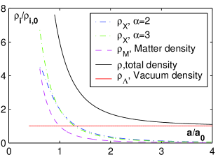
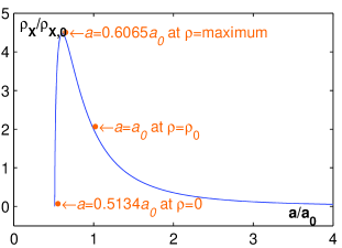
Figure 1 shows
from the zero ECG density point, and with the increasing of scale factor , the dynamically changing part of dark energy density has reached a biggest value (for example: corresponding to case, seeing Figure 2), and then it approaches to a constant near zero.
As to , we gain , which can be described directly by conventional EOS ( is constant). More discussions for this situation can be found in references EB ; LMGB ; MAM , for example.
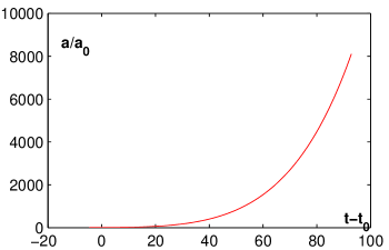
Because the uncertainty of , the above integration is not easy to solve. But for a general picture about the scale factor, we can simply put . Thus we get the integration result:
| (11) |
where . Eq.(11) can be directly figured as in 3, which explicitly shows scale factor in a accelerating state with and there is no singularity during the process.
Since no singularity(see reference SN for the classification of singularity) occurs during the evolution of , we can discuss the crossing with it. So far as we know, results in the following equations with subscript denoting today’s value:
| (12) |
where is defined by called Judge for its following property.
Taking (10)into above equation, we can get:
Then we can see that through the evolution of scale factor , the value of state parameter changes continuously. So that crossing state barrier would occur during the procedure of the evolution. It has also told that Judge here played an important role of relating to the different ranges of the present state parameter and the scale factor (denoted by ) in accordance with Phantom Divide() crossing as tabled in II.1 below.
| Table II.1. Parameter ranges and | ||
Why can the Judge have such important property? In the next part, we will work out its physical meaning in the more complete background.
Now, as for eq.(2), we can get its equivalent expression as:
| (13) | |||||
where with is reduced Hubble parameter and is red-shift, , , , and (, , , and are, respectively, present non-relative matter density, dynamically changing part dark energy density, Hubble parameter, and scale factor); is the current critical density. These density parameters should satisfy the following relation:
| (14) |
Previously, we have pointed out that at the stage of the density evolves like dust-like matter and now we can also see this point from following. Around , we can expand the term around , and preserve the first order of and plus other terms. Thus, we get:
| (15) | |||||
The equivalent density parameter now is defined by:
| (16) |
which has included the dark energy density contribution part. The term corresponds to the radiation component, which can be neglected in the beginning.
Considering the deceleration parameter , it can be expressed by the use of reduced Hubble parameter as:
| (17) |
Therefore, ( is the present deceleration parameter). Evaluating from Eq.(13) and solving with respect to , we get:
| (18) |
So far, the physical meaning of parameter term has clearly stood before us. It reflects the combination of density parameters and deceleration parameter at present. In other words, if we know the values of density parameters and deceleration parameter, we would know the ranges of and . In addition, from Eq.(18), we also know: .
II.2 The case
In this section, we have and Eq.(9) has the following result:
| (19) |
where is defined by called reduced scale factor. We can see that dynamically changing part dark energy density evolves depending on two terms of and , and the values of pure parameters term determine the effect. Additionally, the equation (19) also tells us that decreases while the scale factor increases.
Combined with the EOS , the state parameter is expressed as:
| (20) |
. Taking (19) into consideration, we can get the following relation:
Through the evolution of scale factor , the value of would satisfy the above relation, that is, the crossing phenomenon would occur. The different ranges of the present state parameter and the scale factor corresponding to the state barrier() can be shown from the following table no matter whether or .
| Table II.2. Parameter ranges and | ||
Note: it is similar to table II.1, but the Judge has changed.
Corresponding to Eq.(13), we can write out the expression of the case as:
| (21) | |||||
It would be interesting to discuss the behavior around . Thus, we can expand the around , preserve the first order of , and get:
| (22) | |||||
where is defined by
| (23) |
The effective matter component also gets the contribution from the dark energy component.
With the use of Eq.(17), we can get the Judge as:
| (24) |
It results in: which is quite different from case, and this difference can be used as to distinguishing the two cases.
III Remarks on
In the above treatment a as in the last section is just one of the possible forms for . Generally, we are not able to obtain directly from theoretical analysis. However, as to the far future universe in which (here we also define ) will approach to zero with redshift negative if we define today’s redshift value as zero, the behaviour of is then determined by the small quantity . It is natural to think of Taylor series expansion. We substitute by for simplification, and then expand .
Taking it into the expression of EOS, the pressure becomes
| (25) |
Compared with , the above expression is a combination of Eq.(5) with different values of . This property may also imply that at the different cosmic stages there is an accordant effective value of in the EOS (refeq:state equation) to describe the dark energy fluid. As for far future stage, takes zero after neglecting small quantities.
Calculating density from Eq.(9), we get
Often, and depend on each other and we can deduce out the interrelationship of them from integration formula(9). Thus, pressure can be at last expressed as a function with one variable , for example, , but not the two variables function . As for EOS , and are both used to determine and at last has no relation with . According to this assumpation, we would try to choose to satisfy this requirment. Through a series of analysis, we finally get
where is a lower limit for density as following. Thus, becomes
where and is the density lower limit defined by
As a result, the EOS
| (26) |
is irrelevant to . Then, we will discuss what information about universe this EOS gives.
III.1 The expansion of universe
For the purpose to show the extended Chaplygin gas contribution, we can temporally neglect and in Eq.(2) and assume the universe is flat for simplification. Solve Eq.(2) and get
| (27) |
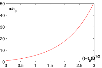
where and is the present scale factor and age of universe, respectively. This function can easily be shown in figure 4, on which the reduced scale factor increases accompanying the elapse of cosmic time. And also implies our universe at the acceleration phase of state.
III.2 contributions from dynamical dark energy
Under the help of Eq.(2), reduced Hubble parameter can take the following form:
| (28) | |||||
As for ‘-term’ in above formula, it is easy to deploy to get , , and constant terms. Then combined them with the other terms, we can get:
| (29) | |||||
where
, ,and are the effective density parameters and show the -term behaviors. Noting our prerequisite at cosmic far future evolution stage, the reduced Hubble parameter can be approximately written as
which means the de sitter phase. If our prerequisite is not so strict, we can see that for the bigger values of , that means a dust-like phase. On the whole , our universe has experienced a phase transition from dust-like stage to a de sitter stage during the process of cosmic evolution.
III.3 The crossing problem
In section two we have discussed the crossing problem in general cases, and now we reconsider it with the specific situation. Taking EOS into the state parameter formula , we get:
| (30) |
It is obvious that , that is to say, there is no crossing phenomenon in this specific model and this particular case belongs to a quintessence-like dark energy.
IV Conclusion and discussion
In this paper, in order to discuss the properties of dark energy with more possibilities, which is used to explain currently cosmic accelerating expansion, we have extended the Chaplygin gas model by which the Dark Fluid concept can be realized with its contributions to effective universe compositions. Through a series of mathematical treatment, it shows that there are indeed some cases that can realize state parameter crossing. Moreover, the physical meanings behind the parameter terms like in Sec.II.1 are interpreted.
Firstly, as for the case, we find that first increases a maximum, and then decreases approaching to a constant near . During the procedure, the pressure decreases to . At the neighborhood of , the behavior of the density is similar to non-relative matter with . With further analysis, we find that the state parameter can cross its traditional barrier smoothly without singularity. By the calculations of the reduced Hubble parameter (15), we find that the dynamically changing part of dark energy density is effectively equivalent to the sum of the matter-like part and radiation-like part. After considering the deceleration parameter , the parameter term is explicitly expressed as combination of the present density parameters (subscript ) and the present deceleration parameter .
Secondly, as to the case, mostly it is similar to the case. However, different from the former case, the density is made up of -term and -term, and it is equivalent to total effects of both a non-relative matter and some kinds of dark energy fluid with density . Obviously, from Eq.(19) always decreases to approach zero with the scale factor increasing.
Thirdly, after describing the general situations, we also discuss a set of specific values of . Then, with parameter independent assumpation, concrete calculations show that the universe is in the state of accelerating expansion with . At last, we compare our model with the typical state parameter obtaining , which means that there is never crossing phenomenon in this case. By discussing the reduced Hubble parameter , we know that the dark energy fluid is evolving equivalently to a fluid with .
To sum up, we have discussed the extended Chaplygin gas model in detail, with the hope to show more possible properties for dark energy and to realize the concept of Dark Fluid for a suggestive describing the cosmic dark components. To constrain the EOS characterizing parameters, work will be done to maximize the following likelihood function(see reference SC ):. And also in this paper, interactions between the different components of cosmology are not considered. We will publish the contents elsewhere soonmhr .
V Acknowledgement
We thank Prof.S.D.Odintsov for reading the manuscript with helpful comments and Profs. I. Brevik and Lewis H.Ryder for lots of interesting discussions. This work is partly supported by NSF and Doctoral Foundation of China.
References
- (1) Special section in Science 300(2003)1893
- (2) D.N.Spergel et al., Astrophys.J.Suppl. 148 (2003) 175.
- (3) M.Tegmark et al., Phys.Rev.D 69 (2004) 103501.
-
(4)
A.G.Riess et al., Astron.J. 116 (1998) 1009;
S.perlmutter et al., Astrophys.J. 517 (1999) 565. - (5) Particle Data Group, Phys.Lett.B592(2004)
- (6) X.Zhang, et al, astro-ph/0411221; Z.K. Guo and Y.Z. Zhang(2005), astro-ph/0506091; G.Sethi, et al, astro-ph/0508491.
- (7) S.Nojiri and S.D.Odintsov, PLB571,2003,1; S.Nojiri and S.D. Odintsov, PRD 70,2004,103522 ; S.Nojiri and S.D. Odintsov, Phys.Rev.D, 2005.
- (8) David Polarski and Andre Ranquet, arxiv: astro-ph/0507290(preprint).
- (9) W. Hu, astro-ph/0410680.
-
(10)
Alexander Kamenshchik, Ugo Moschella, Vincent
Pasquier, Phys.Lett.B 511 (2001) 265-268;
V. Gorini, A. Kamenshschik and U. Moschella, Phys. Rev. D67 (2003) 063509. - (11) N.Bilic, G.B.Tupper, and R.D.Viollier, Phys.Lett.B 535, 17 (2002), astro-Ph/0111325.
- (12) M.C.Bento, O.Bertolami, and A.A.Sen, Phys.Rev.D 66, 043507 (2002), gr-qc/0202064.
- (13) E Babichev, V Dokuchaev and Yu Eroshenko, Class.Quantum Grav.22(2005) 143-154
- (14) L.M.G. Beça and P.P. Avelino(2005), astro-ph/0507075.
-
(15)
Melchiorri A, Mersini L, Odman C J and Trodden M
2003 Phys.Rev.D 68 043509
Choudhary T R and Padmanabhan T 2003 astro-ph/0311622 - (16) S. Nojiri, S. D. Odintsov, Phy. Rev. D 70, 103522(2004) arxiv: hep-th/0408170.
- (17) Luis P. Chimento, Ruth Lazkoz, arxiv: astro-ph/0505254.
- (18) Hao JG and Li XZ 2004 astro-ph/0208465.
-
(19)
B.Ratra and P.J.E.Peebles, Phys.Rev.D 37(1988) 3406;
C.Wetterich, Nucl. Phys.B 302 (1988) 668. -
(20)
I.Zlatev, L.M.Wang and P.J.Steinhardt, Phys.Rev.Lett.
82 (1999) 896;
P.J.Steinhardt, L.Wang and I.Zlatev, Phys.Rev.D 59 (1999) 123504. - (21) J.Hoppe, hep-th/0003288.
- (22) R.Jackiw, A.P.Polychronakos, Phys.Rev.D 62 (2000) 085019.
- (23) S.Capozziello, V.F. Cardone, E.Elizalde, and so on 2005 asto-ph/0508350.
- (24) X.Meng, M.Hu and J.Ren, in preparation