The State Equation of Yang-Mills Field Dark Energy Models
Abstract
In this paper, we study the possibility of building Yang-Mills(YM) field dark energy models with equation of state (EoS) crossing -1, and find that it can not be realized by the single YM field models, no matter what kind of lagrangian or initial condition. But the states of and all can be naturally got in this kind of models. The former is like a quintessence field, and the latter is like a phantom field. This makes that one can build a model with two YM fields, in which one with the initial state of , and the other with . We give an example model of this kind, and find that its EoS is larger than -1 in the past and less than -1 at the present time. We also find that this change must be from to , and it will go to the critical state of with the expansion of the Universe, which character is same with the single YM field models, and the Big Rip is naturally avoided.
pacs:
98.80.Cq, 98.80.Bp, 04.90.+eI Introduction
Recent observations on the Type Ia Supernova (SNIa)sn , Cosmic Microwave Background Radiation (CMB)map and Large Scale Structure (LSS)sdss all suggest that the Universe mainly consists of dark energy (73%), dark matter (23%) and baryon matter (4%). How to understand the physics of the dark energy is an important mission in the modern cosmology, which has the EoS of , and leads to the recent accelerating expansion of the Universe. Several scenarios have been put forward as a possible explanation of it. A positive cosmological constant is the simplest candidate, but it needs the extreme fine tuning to account for the observed accelerating expansion of the Universe. This fact has led to models where the dark energy component varies with time, such as quintessence modelsquint , which assume the dark energy is made of a single (light) scalar field. Despite some pleasing features, these models are not entirely satisfactory, since in order to achieve (where and are the dark energy and matter energy densities at present, respectively) some fine tuning is also required. Many other possibilities have been considered for the origin of this dark energy component such as a scalar field with a non-standard kinetic term and k-essence modelsk , it is also possible to construct models which have the EoS of , the so-called phantomphantom . Some other models such as the generalized Chaplygin gas (GCG) modelsGCG , the vector field modelsvec also have been studied by a lot of authors. Although these models achieve some success, some problems also exist. One essential to understand the nature of the dark energy is to detect the value and evolution of its EoS. The observation data shows that the cosmological constant is a good candidateseljak , which has the effective equation , . However, there is an evidence to show that the dark energy might evolve from in the past to today, and cross the critical state of in the intermediate redshifttrans . If such a result holds on with accumulation of observational data, this would be a great challenge to the current models of dark energy. It is obvious that the cosmological constant as a candidate will be excluded, and dark energy must be dynamical. But the normal models such as the quintessence fields, only can give the state of . Although the k-essence models and the phantom models can get the state of , but the behavior of crossing can not be realized, and all these will lead to theoretical problem in field theory. To answer this crossing phenomenon of , a lot of people have advised some more complex models, such as the quintom modelsquintom ; quintom1 , which is made of a quintessence field and a phantom field. The model with higher derivative term has been suggested in Ref.lmz , which also can get from to , but it also will lead to theoretical difficulty in field theory.
We have advised that the YM fieldZhang ; zhao can be used to describe the dark energy. There are two major reason that prompt us to study this system. First the normal scalar models the connection of field to particle physics models has not been clear so far. The second reason is that the weak energy condition can not be violated by the field. The YM field we have advised has the desired interesting featured: the YM field are the indispenable cornerstone to any particle physics model with interactions mediated by gauge bosons, so it can be incorporated into a sensible unified theory of particle physics. Besides, the EoS of matter for the effective YM condensate is different from that of ordinary matter as well as the scalar fields, and the state of and can also be naturally realized. But if it is possible to build a YM field model with EoS crossing ? In this paper, we focus on this topic. First we consider the YM field with a general lagrangian, and find the state of is easily realized, as long as it satisfies some constraint. From the kinetic equation of the YM field, we find that with the expansion of the Universe. But no matter what kind of lagrangian and initial condition we choose, this model can not get a behavior of crossing . But it can be easily got in the models with two YM fields, one with the initial condition of , which is like a quintessence field, and the other with like a phantom field.
This paper is organized as follows. In section 2 we discuss the general YM field model, and study the evolution of its EoS by solving its kinetic equation. But we find that this kind of model can not get the state of crossing . Then we study the two YM fields model in section 3, and solve the evolution of with scale factor for an example model. We find that crossing can be easily realized in this model, which is very like the quintom models. At last, we have a conclusion and discussion in section 4.
II Single YM Field Model
In the Ref.zhao , we have discussed the EoS of the YM field dark energy models, which has the effective lagrangianpagels ; adler
| (1) |
here plays the role of the order parameter of the YM condensate, and is the running coupling constant which, up to 1-loop order, is given by
| (2) |
Thus the effective lagrangian is
| (3) |
where . for the generic gauge group is the Callan-Symanzik coefficientPol , is the renormalization scale with the dimension of squared mass, the only model parameter. The attractive features of this effective YM action model include the gauge invariance, the Lorentz invariance, the correct trace anomaly, and the asymptotic freedompagels . With the logarithmic dependence on the field strength, has a form similar to he Coleman-Weinberg scalar effective potentialcoleman , and the Parker-Raval effective gravity lagrangianparker .
It is straightforward to extend this model to the expanding Robertson-Walker (R-W) spacetime. For simplicity we will work in a spatially flat R-W spacetime with a metric
| (4) |
where we have set the speed of light , denoting the background space is flat, and is the conformal time. Consider the dominant YM condensate minimally coupled to the general relativity with the effective action,
| (5) |
where is the determinant of the metric . By variation of with respect to the metric , one obtains the Einstein equation , where the energy-momentum tensor is given by
| (6) |
The dielectric constant is defined by , and in this one-loop order it is given by
| (7) |
This energy-momentum tensor is the sum of the several different energy-momentum tensors of the vectors, , neither of which is of prefect-fluid form, which can make the YM field being anisotropy. This is one of the most important character of the vector field dark energy modelsvec . If it is true and this anisotropy YM field is dominant in the Universe, this will make the Universe being anisotropy, one would expect an anisotropy expansion of the Universe, in conflict with the significant isotropy of the CMBisotropy . But on the other hand there also appear to be hints of statistical anisotropy in the CMB perturbationsfluctuate . But here we only consider the other case. For keeping the total energy-momentum tensor is homogeneous and isotropic, here we assume the gauge fields are the functions of only time , and (here are the Pauli’s matrices) are given by and . Define the YM field tensor as usual:
| (8) |
where is the structure constant of gauge group and for the case. This tensor can be written in the form with the electric and magnetic field as
| (9) |
It can be easily found that , and . Thus has a simple form with , where and . In this case, each component of the energy-momentum tensor is
| (10) |
| (11) |
Although this tensor is not isotropic, its value along the direction is different from the one along the directions perpendicular to it. Nevertheless, the total energy-momentum tensor has isotropic stresses, and the corresponding energy density and pressure are given by (here we only consider the condition of )zhao
| (12) |
and its EoS is
| (13) |
It is easily found that at the critical point of , which follows that , the Universe is exact a de Sitter expansion. Near this point, if , we have , and follows . So in these models, the EoS of and all can be naturally realized.
For studying the evolution of this EoS, we should solve the YM field equations, which is equivalent with solving the Einstein equationzhao . By variation of with respect to , one obtains the effective YM equations
| (14) |
For we have assumed the YM condensate is homogeneous and isotropic, from the definition of , it is easily found that the component of YM equations is an identity and the spatial components are:
| (15) |
If , this equation is also an identity. When , this equation follows thatzhao ,
| (16) |
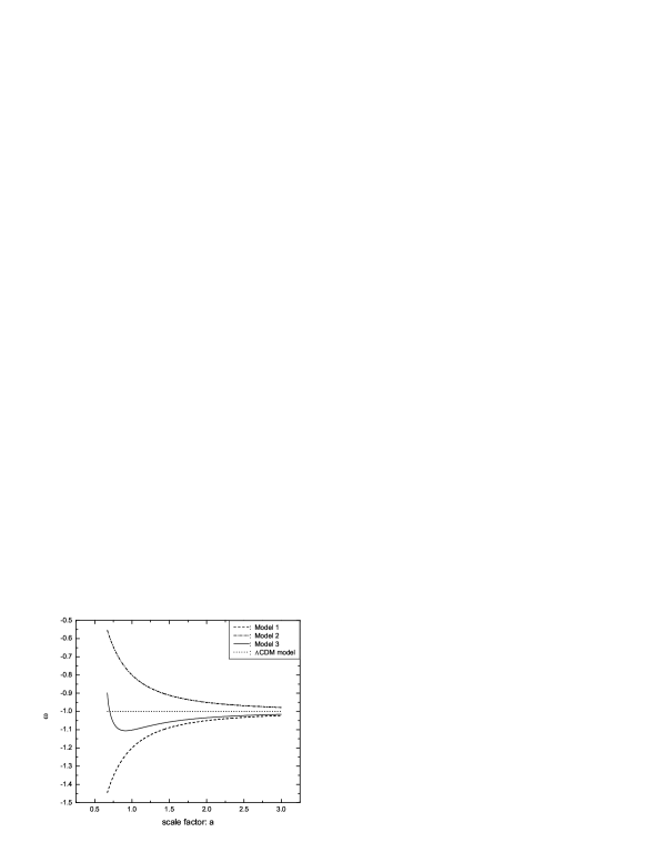
where we have defined , and used the expression of in Eq.(7). In this equation, the proportion factor can be fixed by the initial condition. This is the main equation, which determines the evolution of , and directly relate to the EoS of the YM field. Combining the Eqs.(13) and (16), one can obtains the evolution of EoS in the YM field dark energy Universe. In Fig.[1], we plot the the evolution of in the YM field dark energy models with the present value and , and find that the former one is very like the evolution of the phantom field, and the latter is like a quintessence field. They all have same attractor solution with . So in these models, the Big Rip is naturally avoided. This is the most attractive feature of the YM field models.
In the Eq.(16), the undetermined factor can be fixed by the present value of EoS , which must be determined by observations on SNIa, CMB or LSS. In this paper, we will only show that the observation of CMB power spectrum is an effective way to determine it. The dark energy can influence the CMB temperature anisotropy power spectrum (especially at the large scale) by the integral Sachs-Wolfe(ISW) effectisw . Consider the flat R-W metric with the scalar perturbation in the conformal Newtonian gauge,
| (17) |
The gauge-invariant metric perturbation is the Newtonian potential and is the perturbation to the intrinsic spatial curvature. Always the background matters in the Universe are perfect fluids without anisotropic stress, which follows that . So there is only one perturbation function in the metric of (17), and its evolution is determined byevolution
| (18) |
where , and the ′prime′ denotes . The pressure , and energy density , which should include the contribution of baryon, photon, neutron, cold dark matter, and the dark energy. Especially at late time of the Universe, the effect of the dark energy is very important. We remind that the ISW effect stems from the time variation of the metric perturbations,
| (19) |
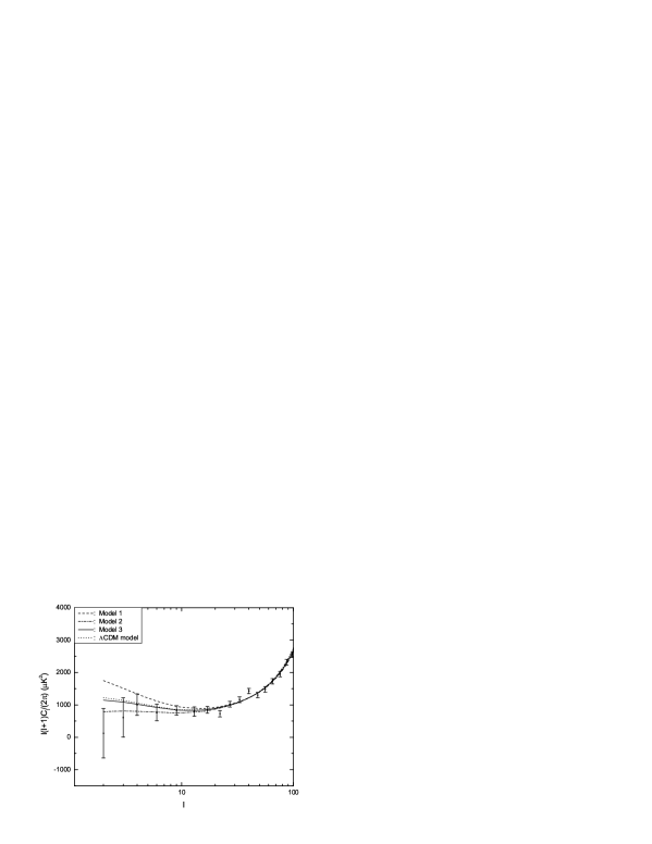
where is the conformal distance to the last scattering surface and the th spherical Bessel function. The ISW effect occurs because photons can gain energy as they travel through time-varying gravitational wells. One always solves the CMB power spectrum in the numerical methodscmbfast ; camp . In Fig.[2], we plot the CMB power spectrum at large scale with these two kind of YM dark energy models, where we have chosen the cosmological parameters as: the Hubble parameter , the energy density of baryon , and dark matter , the reionization optical depth , the spectrum index and amplitude of the primordial perturbation spectrum being without running and . Where we haven’t consider the perturbation of the dark energy. From this figure, one can find that the values of the CMB power spectrums are very sensitively dependent on . Comparing with the CDM model (which is equivalent with the YM model with ), the model with , which is like the quintessence field model, the CMB spectrums have smaller values, especially at scale of , the difference is very obvious; but the model with , which is like the phantom field model, the CMB spectrums have larger values. For the evolution of EoS is only determined by the , the value of it can be determined by fitting the CMB observation. It is obvious that the recent observations on the CMB power spectrums at large scale from WMAP satellite have large error. The further results will depend on the observation of the following WMAP and Planck satellites.
Now let’s return to the evolution of . From Fig.[1], one finds that crossing can not be realized in these models with a single YM field, no matter what values of we have chosen. For studying it more clear, assume the YM field has an initial state of , which follows that , the Eq.(16) becomes
| (20) |
The value of will go to zero with the expansion of the Universe. This means that will go to a critical state of . And the EoS is
| (21) |
This result has two important characters: i) with the expansion of the Universe, will go to the critical point of . This is the most important character of this dark energy model, which is very like the behavior of the vacuum energy with ; ii) the value of and all can realized, but it can not cross from one area to another. This character is same with the scalar field such as the quintessence field, the k-essence and the phantom field models.
It is interesting to ask: if these characters are correct just for the YM model with the lagrangian as formula (3)? Whether or not one can build a model, whose EoS can cross ? So let’s consider the YM field model with a general effective lagrangian as:
| (22) |
where is the running coupling constant, which is a general function of . If we choose , this effective lagrangian returns to the from in Eq.(3). The dielectric constant also can be defined by , which is
| (23) |
Here represents . We also discuss the homogeneous and isotropy YM field with electric field , then the energy density and the pressure of the YM field are:
| (24) |
| (25) |
The energy density follows a constraint . The EoS of this YM field is
| (26) |
where we have defined that . When the condition of can be got at some state with and , the state of is naturally realized. This condition can be easily satisfied. In the discussion as below we only consider these kind of YM fields. For example, in the model with the lagrangian (3), is got at the state . Near this state, leads to , and leads to . But if the YM field has a trivial lagrangian with , which follows that , and . This is exactly the EoS of the relativistic matter, and it can not generate the state of .
To study the evolution of EoS, we also consider the YM equation, which can be got by variation of with respect to ,
| (27) |
from the definition of , it is found that these equations become a simple relation:
| (28) |
where is defined by . If , this equation is an identity, and from (26), we know , which can’t be differentiated from cosmological constant. When , this equation can be integrated to give
| (29) |
For we want to study whether or not the EoS of this YM field can cross , here we assume its initial state is . In this condition, from the expression of and , it follows that , and nearly keep constant, which is for the Universe is nearly de Sitter expansion and is nearly a constant in this Universe. So the YM equation suggests that
| (30) |
From the EoS of (26), one knows that
| (31) |
This is the EoS evolution equation of the general YM field dark energy models. It is exactly same with special case of Eq.(21). So it also keeps the characters of the special case with the lagrangian (3): will run to the critical point with the expansion of the Universe. But it can not cross this critical point. These is the general characters of these kind of YM field dark energy models. For showing this more clear, we discuss two example models.
First we consider the YM field with the running coupling constant
| (32) |
where and are quantity with positive value, and is a positive number. The constraint of follows that
| (33) |
The dielectric constant can be easily get
| (34) |
and
| (35) |
It is obvious that when , is satisfied, and which leads to . Near this critical state, . So the YM equation of (29) becomes
| (36) |
which follows that . From the expression of in Eq.(26), one can easily get
| (37) |
This is exact same with the evolution behavior shown in formula (31).
Another example, we consider the YM field with the coupling constant of
| (38) |
where the constant quantity . When , this lagrangian becomes the trivial case with , but when is near , the nonlinear effect is obvious. Then
so the critical state of leads to and . By the similar discussion, from the YM field (29), one can also get near this critical state, which generates .
III Two YM Fields Model
In the former section, we have discussed that the dark energy models with single YM field can’t form a state of crossing , not matter what kind of lagrangian or initial condition. But we should notice another character: the YM field has the EoS of , when its initial value is near the critical state of . So if the YM field has an initial state of , it will keep this state with the evolution of the Universe, which is like the quintessence models. But if its initial state is , it will also keep it, which is like the phantom models. This makes that we can build a model with two different free YM fields, one having an initial state of and the other being . In this kind of models, the behavior of crossing is easily got. This idea is like the quintom modelsquintom , where the authors built the model with a quintessence field and a phantom field.
In the below discussion, we will build a toy example of this kind of model. Assume the dark energy is made of two YM fields with the effective lagrangian as Eq.(3)
| (39) |
where , and . Their dielectric constants are
| (40) |
From the YM field kinetic equations, we also can get the relations:
| (41) |
where are the integral constant, which are determined by the initial state of the YM fields. If the YM field is a phantom like field with , then and . At the same time, a quintessence like YM field follows that . Here we choose the YM field of as the phantom like field with , and as the quintessence like field with . The energy density and pressure are
| (42) |
so the total EoS is:
| (43) |
where we have also defined that . Using the relation of and , we can simplify the equation of state as
| (44) |
where . We need this dark energy has the initial state of , which requires that the field of is dominant at the initial time. This is easily obtained as long as at this time is satisfied. The finial state, we need to get , which means that is dominant, and the behavior of crossing realized in the intermediate time. But how to get this? From the before discussion, we know in the Universe with only one kind of YM field (i=1 or 2), the YM equation follows that . And it will go to the critical state with the expansion of the Universe. At this state, , and keeps constant. So in this two YM fields model, if we choose the condition , this may follow that the finial energy density , and is dominant. For this intent, we build this model with the condition as below: choosing , which can ensure the finial state, the first kind of YM field is the dominant matter. At the present time, corresponding to the scale factor , we choose that and , which keeps that the first field always having a state of (like the phantom) and the second field with (like the quintessence). These choice of leads to the present EoS
| (45) |
which is like the phantom field. Since increases, and decreases with the expansion of the Universe, there must exist of a time, before which is dominant, and this leads to the total EoS at that time.
Combining the Eqs.(41) and (44), we can solve the evolution of EoS with the scale time in numerical calculation, where the relation of and is easily got
For each kind of YM field, its EoS is
| (46) |
The condition of will generate . The evolution of them are shown in Fig.[3]. This is exact result we expect, runs to the critical point of with the expansion of the Universe, which makes runs to , no matter what kind of initial values. This is same with the single YM field model. With , the strength of the field will also go to its critical point . This can be shown in Fig.[4]. For we have chosen the condition of , it must lead to at some time, the first kind of YM field becomes dominant, and the total EoS is realized. This can be shown in Fig.[1]. In Fig.[2], we also plot the CMB power spectrum in the Universe with this kind of YM field dark energy, and find that it is difficult to be distinguished from the CDM Universe, which is for the effect of the dark energy on the CMB power spectrum is an integral effect from CMB decoupling time to now. But the evolution detail of is not obvious. This is the disadvantage of this way to detect dark energy.
Now, let’s conclude this dark energy model, which is made of two YM fields. One has the EoS of and the other is . At the initial time, we choose their condition to make , and second kind of YM field is dominant, which makes the total EoS at this time. This is like the quintessence model. For the keeps for all time, from the Friedmann equations, one knows that its energy density will enhance with the expansion of the Universe. And at last it will run to its critical point . And the same time, will decrease to its critical state . For we have chosen , which must make and some time, and after this, is dominant, the total EoS . So the equation of state crossing is realized. It is simply found that this kind of crossing must be from to , which is exactly same with the observations. But the contrary condition, from to can’t be realized in this kind of models.
IV Conclusion and Discussion
In summary, in this letter we have studied the possibility of crossing in the YM field dark energy models, and found that the single YM field models can not realize, no matter what kind of their effective lagrangian, although this kind of models can naturally give a state of or , which depends on their initial state. Near the critical state of , the evolution of their EoS with the expansion of the Universe is same, , which means that the Universe will be a nearly de Sitter expansion. This is the most attractive character of this kind of models, and this makes it very like the cosmological constant. So the Big Rip is naturally avoided in this model. But this evolution behavior also shows that the single field models can not realize crossing . This is same with the single scalar field models.
But in these models, and all can be easily got. The former behavior is like a quintessence field, and the later is like a phantom field. So one can build a model with two YM fields, and one field with and the other with . This idea is very like the quintom models. Then we give an example model and find that in this model, the property of crossing the cosmological constant boundary can be naturally realized, and we also found that this crossing must be from to , which is exact the observation result. In this model, the state will also go to the critical state of with the expansion of the Universe, as the single YM field models. This is the main character of the YM field dark energy models, which makes the Big Rip is avoided. The present models we discuss in this paper are in the almost standard framework of physics, e.g. in general relativity in 4-dimension. There does not exist phantom or higher derivative term in the model, which will lead to theory problems in field theory. Instead, the YM field as (3), is introduced, which includes the gauge invariance, the Lorentz invariance, the correct trace anormaly, and the asymptotic freedom. These are the advantages of this kind of dark energy models. But these models also exist some disadvantages: first, what is the origin of the YM field? and why its renormalization scale is so low as the present density of the dark energy? In the two YM fields model, we must choose to realize the crossing , which is a mild fine-tuning problem. All these make this kind of models being unnatural. These are the universal problems which exist in most dark energy models. If considering the possible interaction between the YM field and other matter, especially the dark matter, which may have some new characterzhang2 . This topic had been deeply discussed in the scalar field dark energy modelsinter , but had not been considered in this paper.
Acknowledgements
Y. Zhang’s research work has been supported by the Chinese NSF (10173008) and by NKBRSF (G19990754).
References
- (1) A.G.Riess et al., Astron.J. 116 (1998) 1009; S.Perlmutter et al., Astrophys.J. 517 (1999) 565; J.L.Tonry et al., Astrophys.J. 594 (2003) 1; R.A.Knop et al., astro-ph/0309368;
- (2) C.L.Bennett et al.,Astrophys.J.Suppl. 148 (2003) 1; D.N.Spergel et al.,Astrophys.J.Suppl. 148 (2003) 175; H.V.Peiris et al., Astrophys.J.Suppl. 148 (2003) 213;
- (3) M.Tegmark et al.,Astrophys.J. 606 (2004) 702, Phys.Rev.D 69 (2004) 103501; A.C.Pope et al.,Astrophys.J. 607 (2004) 655; W.J.Percival et al., MNRAS 327 (2001) 1297;
- (4) C.Wetterich, Nucl.Phys.B 302 (1988) 668 ; Astron.Astrophys. 301 (1995) 321; B.Ratra and P.J.Peebles, Phys.Rev.D 37 (1988) 3406; R.R.Caldwell, R.Dave and P.J.Steinhardt, Phys.Rev.Lett. 80 (1998) 1582;
- (5) C.Armendariz-Picon, T.Damour and V.Mukhanov, Phys.Lett.B 458 (1999) 209 ; T.Chiba, T.Okabe and M.Yamaguchi, Phys.Rev.D 62 (2000) 023511 ; C.Armendariz-Picon, V.Mukhanov and P.J.Steinhardt, Phys.Rev.D 63 (2001) 103510 ; L.P.Chimento, Phys.Rev.D 69 (2004) 123517 ; P.F.Gonzalez-Diaz, Phys.Lett.B 586 (2004) 1;
- (6) R.R.Caldwell, Phys.Lett.B 545 (2002) 23; S.M.Carroll, M.Hoffman and M.Trodden, Phys.Rev.D 68 (2003) 023509 ; R.R.Caldwell, M.Kamionkowski and N.N.Weinberg, Phys.Rev.Lett. 91 (2003) 071301 ; M.P.Dabrowski, T.Stachowiak and M.Szydlowski, Phys.Rev.D 68 (2003) 103519 ; V.K.Onemli and R.P.Woodard, Phys.Rev.D 70 (2004) 107301;
- (7) A.Y.Kamenshchik, U.Moschella and V.Pasquier, Phys.Lett.B 511 (2001) 265; N.Bilic, G.B.Tupper and R.D.Viollier, Phys.Lett.B 535 (2002) 17; M.C.Bento, O.Bertolami and A.A.Sen, Phys.Rev.D 66 (2002) 043507;
- (8) C.Armendariz-Picon, JCAP 0407 (2004) 007; V.V.Kiselev, Class.Quant.Grav.21 (2004) 3323; W.Zimdahl, D.J.Schwarz, M.Novello, S.E.Perez Bergliaffa and J.Salim, astro-ph/0312093;
- (9) U.Seljak et al., Phys.Rev.D 71 (2005) 103515;
- (10) P.S.Corasaniti, M.Kunz, D.Parkinson, E.J.Copeland and B.A.Bassett, Phys.Rev.D 70 (2004) 083006; S.Hannestad and E.Mortsell, JCAP 0409 (2004) 001; A.Upadhye, M.Ishak and P.J.Steinhardt, Phys.Rev.D 72 (2005) 063501 ;
- (11) B.Feng, X.L.Wang and X.M.Zhang, Phys.Lett.B 607 (2005) 35;
- (12) W.Hu, Phys.Rev.D 71 (2005) 047301; Z.K.Guo, Y.S.Piao, X.M.Zhang and Y.Z.Zhang, Phys.Lett.B 608 (2005) 177; R.R.Caldwell and M.Doran, Phys.Rev.D 72 (2005) 043527;
- (13) M.Z.Li, B.Feng and X.M.Zhang, JCAP 0512 (2005) 002;
- (14) Y.Zhang, Phys.Lett.B 340 (1994) 18; Class.Quan.Grav.13 (1996) 1 ; Chin.Phys.Lett.14 (1997) 237; 15 (1998) 622; 17 (2000) 76; Gene. Relat. and Grav. 34 (2002) 2155; 35 (2003) 689; Chin.Phys.Lett.20 (2003) 1899;
- (15) W.Zhao and Y.Zhang, astro-ph/0508010;
- (16) H.Pagels and E.Tomboulis, Nucl.Phys.B 143 (1978) 485;
- (17) S.Adler, Phys.Rev.D 23 (1981) 2905; Nucl.Phys.B 217 (1983) 3881;
- (18) H.Politzer, Phys.Rev.Lett. 30 (1973) 1346; D.J.Gross and F.Wilzcek, Phys.Rev.Lett. 30 (1973) 1343;
- (19) S.Coleman and E.Weinberg, Phys.Rev.D 7 (1973) 1888;
- (20) L.Parker and A.Raval, Phys.Rev.D 60 (1999) 063512;
- (21) E.F.Bunn, P.Ferrira and J.Silk, Phys.Rev.Lett. 77 (1996) 2883;
- (22) A.de Oliveira-Costa, M.Tegmark, M.Zaldarriaga and A.Hamilton, Phys.Rev.D 69 (2004) 063516; C.J.Copi, D.Huterer and G.D.Starkman, Phys.Rev.D 70 (2004) 043515; D.J.Schwarz, G.D.Starkman, D.Huterer and C.J.Copi, Phys.Rev.Lett. 93 (2004) 221301; D.L.Larson and B.D.Wandelt, Astrophys.J. 613 (2004) L85; P.Bielewicz, K.M.Gorski and A.J.Banday, MNRAS 355 (2004) 1283; T.R.Jaffe, A.J.Banday, H.K.Eriksen, K.M.Gorski and F.K.Hansen, Astrophys.J. 629 (2005) L1; K.Land and J.Magueilo, Phys.Rev.Lett. 95 (2005) 071301; K.Land and J.Magueilo, astro-ph/0509752; T.Koivisto and D.F.Mota, astro-ph/0512135;
- (23) R.K.Sachs and A.M.Wolfe, Astrophys.J. 1 (1967) 73;
- (24) R.Bharat and P.J.E.Peebles, Phys.Rev.D 37 (1988) 3406; P.J.E. Peebles and R.Bharat, Astrophys.J. 325 (1988) L17 ; J.Weller and A.M.Lewis, MNRAS 346 (2003) 987; C.P.Ma and E.Bertschinger, Astrophys.J. 455 (1995) 7; C.Gordon and W.Hu, Phys.Rev.D 70 (2004) 083003;
- (25) U.Seljak and M.Zaldarriaga, Astrophys.J. 469 (1996) 437;
- (26) A.Lewis, A.Challinor and A.Lasenby, Astrophys.J. 538 (2000) 473;
- (27) Y.Zhang, Chin.Phys.Lett. 20 (2003) 1899;
- (28) L.Amendola, Phys.Rev.D 60 (1999) 043501; T.Damour and A.M.Polyakov, Nul.Phys.B 423 (1994) 532; W.Zimdahl, D.Pavon and L.P.Chinmento, Phys.Lett.B 521 (2001) L33; L.P.Chimento, A.S.Jakubi, D.Pavon and W.Zimdahl, Phys.Rev.D 67 (2003) 083513; Z.K.Guo and Y.Z.Zhang, Phys.Rev.D 71 (2005) 023501; H.Wei and R.G.Cai, Phys.Rev.D 71 (2005) 043504; Z.K.Guo, R.G.Cai and Y.Z.Zhang, JCAP 0505 (2005) 002; R.G.Cai and A.Wang, JCAP 0503 (2005) 002; H.Wei and R.G. Cai, Phys.Rev.D 72 (2005) 123507;