The evolution of the luminosity functions in the FORS Deep Field from low to high redshift: II. The red bands

We present the redshift evolution of the restframe galaxy luminosity function (LF) in the red r’, i’, and z’ bands as derived from the FORS Deep Field (FDF), thus extending the results published in Gabasch et al. (2004a) to longer wavelengths. Using the deep and homogeneous I-band selected dataset of the FDF we are able to follow the red LFs over the redshift range $0.5<z<3.5$. The results are based on photometric redshifts for 5558 galaxies derived from the photometry in 9 filters achieving an accuracy of $\Delta z/(z_{spec}+1)\leq 0.03$ with only $\sim 1$% outliers. A comparison with results from the literature shows the reliability of the derived LFs. Because of the depth of the FDF we can give relatively tight constraints on the faint-end slope $\alpha$ of the LF: The faint-end of the red LFs does not show a large redshift evolution and is compatible within $1\sigma$ to $2\sigma$ with a constant slope over the redshift range $0.5\mathrel{\hbox to0.0pt{\lower 4.0pt\hbox{\hskip 1.0pt$\sim$}\hss}\raise 1.0pt\hbox{$<$}}z\mathrel{\hbox to0.0pt{\lower 4.0pt\hbox{\hskip 1.0pt$\sim$}\hss}\raise 1.0pt\hbox{$<$}}2.0$. Moreover, the slopes in r’, i’, and z’ are very similar with a best fitting value of $\alpha=-1.33\pm 0.03$ for the combined bands. There is a clear trend of $\alpha$ to steepen with increasing wavelength: $\alpha_{UV\&u^{\prime}}=-1.07\pm 0.04$ $\rightarrow$ $\alpha_{g^{\prime}\&B}=-1.25\pm 0.03$ $\rightarrow$ $\alpha_{r^{\prime}\&i^{\prime}\&z^{\prime}}=-1.33\pm 0.03$. We subdivide our galaxy sample into four SED types and determine the contribution of a typical SED type to the overall LF. We show that the wavelength dependence of the LF slope can be explained by the relative contribution of different SED-type LFs to the overall LF, as different SED types dominate the LF in the blue and red bands. Furthermore we also derive and analyze the luminosity density evolution of the different SED types up to $z\sim 2$.
We investigate the evolution of M^∗ and $\phi^{\ast}$ by means of the redshift parametrization $M^{\ast}(z)=M^{\ast}_{0}+{a}\ln(1+z)$ and $\phi^{\ast}(z)=\phi^{\ast}_{0}(1+z)^{b}$. Based on the FDF data, we find only a mild brightening of M^∗ ($a_{r^{\prime}}\sim-0.8$, and $a_{i^{\prime},z^{\prime}}\sim-0.4$) and decrease of $\phi^{\ast}$ ($b_{r^{\prime},i^{\prime},z^{\prime}}\sim-0.6$) with increasing redshift. Therefore, from $\langle z\rangle\sim 0.5$ to $\langle z\rangle\sim 3$ the characteristic luminosity increases by $\sim$ 0.8, $\sim$ 0.4 and $\sim$ 0.4 magnitudes in the r’, i’, and z’ bands, respectively. Simultaneously the characteristic density decreases by about 40% in all analyzed wavebands. A comparison of the LFs with semi-analytical galaxy formation models by Kauffmann et al. (1999) shows a similar result as in the blue bands: the semi-analytical models predict LFs which describe the data at low redshift very well, but show growing disagreement with increasing redshifts.

1 Introduction

One of the major efforts in extragalactic astronomy is to derive and analyze the restframe galaxy luminosity function in different bandpasses and redshift slices in order to follow the time evolution of the galaxy populations by a statistical approach. This is of particular importance because the energy output at different wavelengths is dominated by stars of different masses. While galaxy luminosities measured in the ultraviolet are sensitive to the energy output of hot, short-living O and B type stars and therefore to ongoing star formation (Tinsley, 1971; Madau et al., 1996, 1998), the optical and NIR luminosities provide constraints on more evolved stellar populations (Hunter et al., 1982). This can be used, in principle, to derive the evolution of basic galaxy properties as the stellar mass function (see e.g. Drory et al., 2005, and references therein), the star formation rate density (see e.g. Pérez-González et al., 2005, and references therein) or the specific star formation rate (see e.g. Feulner et al., 2005, and references therein). The determination of these quantities, however, is based on assumptions, e.g. on the shape of the initial mass function or on the details in modeling the stellar population like age, chemical composition, and star formation history. Hence studying the LF at different wavelengths and cosmic epochs offers a more direct approach to the problem of galaxy evolution.
As the LF is one of the fundamental observational tools, the amount of work spent by different groups in deriving accurate LFs is substantial. Based on either spectroscopic redshifts, drop-out techniques, or photometric redshifts, it has been possible to derive luminosity functions at different redshifts in the ultraviolet & blue band (Baldry et al. 2005; Croton et al. 2005; Arnouts et al. 2005; Budavári et al. 2005; Treyer et al. 2005; see also Gabasch et al. 2004a and references therein), in the red bands (Lin et al., 1996, 1997; Brown et al., 2001; Shapley et al., 2001; Wolf et al., 2003; Chen et al., 2003; Ilbert et al., 2004; Dahlen et al., 2005; Trentham et al., 2005) as well as in the near-IR bands (Loveday, 2000; Kochanek et al., 2001; Cole et al., 2001; Balogh et al., 2001; Drory et al., 2003; Huang et al., 2003; Feulner et al., 2003; Pozzetti et al., 2003; Dahlen et al., 2005).
The evolution of the characteristic luminosity and density of galaxy populations can be analyzed by fitting a Schechter function (Schechter, 1976) to the LF. The redshift evolution of the three free parameters of the Schechter function, the characteristic magnitude M^∗, the density $\phi^{\ast}$, and the faint-end slope $\alpha$ can be used to quantitatively describe the change of the LF as a function of redshift. Unfortunately, the Schechter parametrization of the LF cannot account for possible excesses at the bright and faint end or other subtle shape deviations. Furthermore, the Schechter parameters are highly correlated making it challenging, but not impossible, to clearly separate the evolution of the different parameters (see e.g. Andreon 2004 for a discussion).
The evolution of the LFs is also very suitable to constrain the free parameters of theoretical models (e.g. semi-analytical or smoothed particle hydrodynamics models). Ideally a comparison between model predictions and observations should be done simultaneously for different wavebands (UV, optical, NIR) and for different redshift slices as different stellar populations are involved in generating the flux in the different bands. Therefore, the FDF (Heidt et al., 2003) provides a unique testing ground for model predictions, as the depth and the covered area allow relatively precise LF measurements from the UV to the z’-band up to high redshift in a very homogeneous way.
In this paper we extend the measurements of the blue luminosity functions presented in Gabasch et al. (2004a, hereafter FDFLF I) to the red r’, i’, and z’ bands. In Sect. 2 we derive the LFs and show the best fitting Schechter parameters M^∗, $\phi^{\ast}$, and $\alpha$ in the redshift range $0.5<z<3.5$. We also present a detailed analysis of the slope of the LF as a function of redshift and wavelength. Furthermore, we analyze the contributions of different SED types to the overall LF and present the evolution of the type dependent luminosity density up to redshift $z\sim 2$. Sect. 3 shows a parametric analysis of the redshift evolution of the LF, whereas a comparison with the LFs of other surveys as well as with model predictions is given in Sect. 4 and in Sect. 5, respectively. We summarize our work in Sect. 6.
Throughout this paper we use AB magnitudes and adopt a $\Lambda$ cosmology with $\Omega_{M}=0.3$, $\Omega_{\Lambda}=0.7$, and $H_{0}=70\,\mathrm{km}\,\mathrm{s}^{-1}\,\mathrm{Mpc}^{-1}$.

2 Luminosity functions in the r’, i’, and z’ bands

The results presented in this paper are all based on the deep part of the I-band selected catalog of the FDF (Heidt et al., 2003) as introduced in FDFLF I. Galaxy distances are determined by the photometric redshift technique (Bender et al., 2001) with a typical accuracy of $\Delta z/(z_{spec}+1)\approx 0.03$ if compared to the spectroscopic sample (Noll et al., 2004; Böhm et al., 2004) of more than 350 objects. To derive the absolute magnitude for a given band (which will be briefly summarized below) we use the best fitting SED as determined by the photometric redshift code, thus reducing possible systematic errors which could be introduced by using k-corrections applied to a single observed magnitude. To account for the fact that some fainter galaxies are not visible in the whole survey volume we perform a $V/V_{max}$ (Schmidt, 1968) correction. The errors of the LFs are calculated by means of Monte-Carlo simulations and include the photometric redshift error of every single galaxy as well as the statistical error (Poissonian error). To derive precise Schechter parameters we limit our analysis of the LF to the magnitude bin where $V/V_{max}\leq 3$. We also show the uncorrected LF in the various plots as open circles. We do not assume any evolution of the galaxies within the single redshift bins, since the number of galaxies and the distance determination based on photometric redshifts would not be able to constrain it. The redshift binning was chosen such that we have good statistics in the various redshift bins and that the influence of redshift clustering was minimized. In order to have good statistics at the bright end (rare objects) of the LF we had to slightly change some of the redshift bins if compared to FDFLF I. The new redshift binning together with the number of galaxies in every bin is shown in Table 1. As can be seen from Table 1, the redshift intervals are approximately the same size in $\ln(1+z)$ and most of the results we are going to discuss in this paper are based on 700 – 1000 galaxies per redshift bin.

Table 1: Number of galaxies in the FDF for the redshift intervals used for computing the LFs. Note that we derive the LF in all redshift bins, but exclude the lowest ($z<0.45$) and highest redshift bin ($z>3.81$) from our analysis of the LF evolution, since the lowest redshift bin corresponds to too small a volume while the $z>3.81$ bin suffers from extrapolation errors.

redshift	number	fraction
interval	of galaxies	of galaxies
0.00 - 0.45	808	14.54 %
0.45 - 0.85	1109	19.95 %
0.85 - 1.31	1029	18.51 %
1.31 - 1.91	880	15.83 %
1.91 - 2.61	816	14.68 %
2.61 - 3.81	718	12.92 %
$>3.81$	196	3.53 %
unknown	2	0.04 %

2.1 The slope of the LF as a function of redshift

Table 2: Slope of the LF for all wavelengths and all redshifts as derived from a 3-parameter Schechter fit.

$z$	$\alpha$ (r’)	$\alpha$ (i’)	$\alpha$ (z’)
0.45 – 0.85	$-$1.37 (+0.04 $-$0.04)	$-$1.37 (+0.04 $-$0.03)	$-$1.39 (+0.04 $-$0.04)
0.85 – 1.31	$-$1.25 (+0.06 $-$0.04)	$-$1.27 (+0.06 $-$0.05)	$-$1.34 (+0.06 $-$0.04)
1.31 – 1.91	$-$1.30 (+0.16 $-$0.09)	$-$1.50 (+0.13 $-$0.10)	$-$1.45 (+0.12 $-$0.09)
1.91 – 2.61	$-$1.01 (+0.15 $-$0.14)	$-$1.03 (+0.17 $-$0.14)	$-$0.97 (+0.17 $-$0.12)
2.61 – 3.81	$-$0.98 (+0.17 $-$0.17)	$-$1.03 (+0.15 $-$0.13)	$-$1.01 (+0.15 $-$0.13)

Table 3: In the upper part of the Table we show the slope $\alpha$ of the luminosity functions for the different wavebands as determined from an error-weighted fit to the data under the assumption that $\alpha(z)=\mathrm{const.}$ In the lower part of the Table we show the best values of $\alpha$ after combining the data of all bands.

filter	$\alpha(z)=const.$
r’	$-1.30\pm 0.05$
i’	$-1.33\pm 0.05$
z’	$-1.35\pm 0.05$
r’ & i’ & z’	$-1.33\pm 0.03$

To investigate the redshift evolution of the faint-end slope of the LF, we fit a three parameter Schechter function (M^∗, $\phi^{\ast}$, and $\alpha$) to the data points. The best fitting slope $\alpha$ and the corresponding $1\sigma$ errors for the 3 wavebands are reported in Table 2 for the various redshift bins.
It can be inferred from Table 2 that there is only marginal evidence for a change of $\alpha$ with redshift (at least up to $z\sim 2$ where we are able to sample the LF to a suitable depth). Under the assumption that $\alpha$ does not depend on redshift, Table 3 (upper part) yields the slopes’ best error-weighted values in the redshift range from $\langle z\rangle\sim 0.65$ to $\langle z\rangle\sim 1.6$ (including also the higher redshift bins changes $\alpha$ only marginally). Since the slopes in all bands are very similar we derive a combined slope of $\alpha_{r^{\prime}\&i^{\prime}\&z^{\prime}}=-1.33\pm 0.03$ (Table 3, lower part).
Almost all of the slopes listed in Table 2 are compatible within $1\sigma-2\sigma$ with $\alpha=-1.33\pm 0.03$. Therefore, we fixed the slope to this value for the further analysis. Please note, that this slope is steeper than for the blue bands ($\alpha_{UV\&u^{\prime}}=-1.07$ and $\alpha_{g^{\prime}\&B}=-1.25$), but it follows the trend observed in FDFLF I: With increasing wavelength the slope steepens, i.e. the ratio of faint to bright galaxies increases. This trend is illustrated best in Fig. 1, where we combine the results derived in FDFLF I with those of this work and plot the wavelength dependence of the LF slope. As we will show in Sect. 2.3, this effect can be explained by the contribution of different galaxy populations to the overall LF in the various wavebands.

2.2 I selection versus I+B selection

We checked the dependence of our results on the selection band by comparing the I band selected catalog and the I+B selected FDF catalog. The combined catalog has been described in Heidt et al. (2003) and reaches limiting magnitudes of $I\sim 26.8$ and $B\sim 27.6$. In the combined sample $M^{\ast}$ agrees within its $1\sigma$ errors with the values derived from the I-band catalog only. The slope $\alpha$ tends to be slightly steeper in the combined sample, but by not more than $1\sigma$. The larger number of objects in the combined catalog mostly influences the characteristic density $\phi^{\ast}$ which is a factor of 1.05 to 1.20 larger (depending on the redshift bin). Given the errors of $\phi^{\ast}$, this is in the order of $1\sigma$ to $2\sigma$.

2.3 The slope of the LF as a function of wavelength

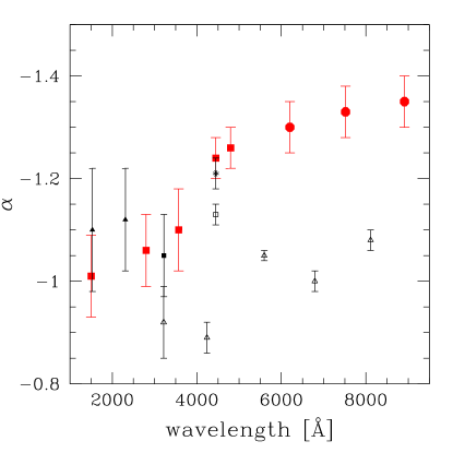
Figure 1: Slope of the LF as a function of wavelength. The filled red squares denote the values derived in FDFLF I whereas the filled red dots are taken from this work (Table 3, upper part). Local slope values (black) are shown as filled squares (Baldry et al., 2005), open squares (Driver et al., 2005), filled triangles (Budavári et al., 2005), open triangles (Blanton et al., 2003), and as an asterisk (Norberg et al., 2002).

Figure 2: SEDs grouped according to their spectral type. See text for details.

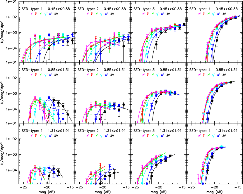
Figure 3: LFs for the four SED types in the redshift intervals $0.45<z\leq 0.85$ (upper panels), $0.85<z\leq 1.31$ (middle panels), and $1.31<z\leq 1.91$ (lower panels): SED type increases from left to right. The filters are color coded and denoted in the upper part of the various panels. For clarity, the three parameter Schechter function fit to the data is shown as solid line with the same color coding as the LF.

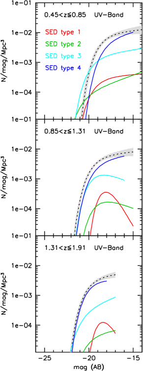
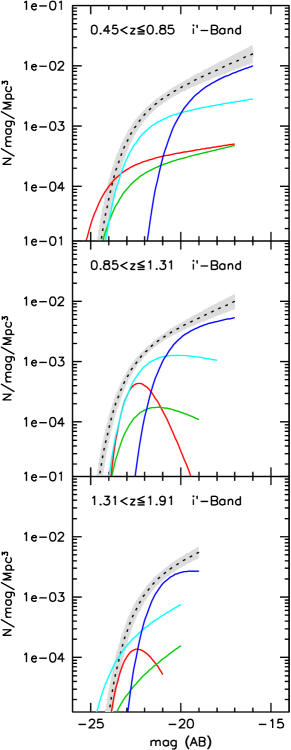
Figure 4: Schechter functions fitted to the LFs in the UV (left panels) as well as in the i’-band (right panels) for the redshift intervals $0.45<z\leq 0.85$ (upper panels), $0.85<z\leq 1.31$ (middle panels), and $1.31<z\leq 1.91$ (lower panels). The solid lines show the best fitting Schechter functions for the four SED types. The SED type is color coded and denoted in the upper left panel. The dotted black line shows the total LF (as fitted to the data) whereas the shaded region represent the corresponding 1$\sigma$ error of the latter. For the slope values of the different SED types see Table 5. Please note that we show the SED type LFs to the limiting magnitude where the $V/V_{max}$ begins to contribute by at most a factor of 1.5, being more conservative than for the overall LF for which we allow a correction factor of 3.

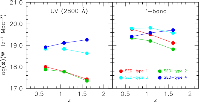
Figure 5: Luminosity densities in the UV (left panel) and i’ (right panel) bands for the four SED types in the redshift intervals $0.45<z\leq 0.85$, $0.85<z\leq 1.31$, and $1.31<z\leq 1.91$. The luminosity densities are completeness corrected to zero luminosity (ZGL, see text for details). The values are listed in Table 4

Table 4: Luminosity densities in the UV and i’ bands for the four SED types. See also Fig. 5

filter	SED type	redshift	luminosity density	error	completeness correction (ZGL)
			W Hz-1 Mpc-3	W Hz-1 Mpc-3	%
UV (2800Å)	1	0.45 – 0.85	1.01e+18	1.5e+17	0.1
		0.85 – 1.31	6.16e+17	1.0e+17	0.7
		1.31 – 1.91	2.68e+17	7.6e+16	8.9
	2	0.45 – 0.85	7.58e+17	1.3e+17	0.5
		0.85 – 1.31	6.00e+17	1.2e+17	2.0
		1.31 – 1.91	2.26e+17	7.0e+16	9.0
	3	0.45 – 0.85	6.88e+18	7.9e+17	0.6
		0.85 – 1.31	6.86e+18	5.4e+17	2.0
		1.31 – 1.91	4.27e+18	5.6e+17	4.7
	4	0.45 – 0.85	8.29e+18	5.1e+17	8.4
		0.85 – 1.31	1.30e+19	8.4e+17	6.9
		1.31 – 1.91	1.83e+19	1.9e+18	21.4
i’	1	0.45 – 0.85	5.72e+19	8.7e+18	0.3
		0.85 – 1.31	3.22e+19	5.4e+18	1.5
		1.31 – 1.91	1.29e+19	3.5e+18	10.2
	2	0.45 – 0.85	2.24e+19	3.9e+18	0.8
		0.85 – 1.31	1.61e+19	3.2e+18	3.6
		1.31 – 1.91	6.60e+18	1.6e+18	11.6
	3	0.45 – 0.85	6.21e+19	6.9e+18	0.4
		0.85 – 1.31	6.56e+19	5.1e+18	1.6
		1.31 – 1.91	3.79e+19	5.4e+18	7.4
	4	0.45 – 0.85	2.59e+19	1.5e+18	5.8
		0.85 – 1.31	3.84e+19	2.4e+18	5.7
		1.31 – 1.91	5.17e+19	4.5e+18	18.9

Table 5: Slope of the UV (2800 Å ) and i’ band LF for the different SED types from a 3-parameter Schechter fit. The Schechter functions are shown in Fig. 4

$z$	filter	$\alpha$ for SED type 1	$\alpha$ for SED type 2	$\alpha$ for SED type 3	$\alpha$ for SED type 4
0.45 – 0.85	UV	$-$1.06 (+0.16 $-$0.10)	$-$1.27 (+0.08 $-$0.04)	$-$1.12 (+0.11 $-$0.07)	$-$1.19 (+0.13 $-$0.11)
0.45 – 0.85	i’	$-$1.11 (+0.15 $-$0.02)	$-$1.17 (+0.22 $-$0.03)	$-$1.12 (+0.12 $-$0.11)	$-$1.23 (+0.07 $-$0.10)
0.85 – 1.31	UV	+0.38 (+0.60 $-$0.37)	$-$0.71 (+0.62 $-$0.27)	$-$0.68 (+0.17 $-$0.15)	$-$1.14 (+0.12 $-$0.08)
0.85 – 1.31	i’	+1.04 (+0.65 $-$0.68)	$-$0.62 (+0.79 $-$0.32)	$-$0.84 (+0.15 $-$0.13)	$-$1.09 (+0.11 $-$0.06)

To better understand the filter-dependence of the LF slope shown in Fig. 1, we analyze the contribution of different galaxy types to the overall LF. Thus, we subdivide our galaxy sample into four SED types and analyze the type-dependent LF, i.e. we determine the contribution of a typical SED type to the overall LF. The SEDs are mainly grouped according to the UV-K color (see Fig. 2): for increasing spectral type (SED type 1 $\rightarrow$ SED type 4) the SEDs become bluer, i.e. the UV flux (and thus the recent star formation rate) increases if compared to the K-band flux. Pannella et al. (2005) analyzed the morphology of about 1400 galaxies in the FDF down to $I\sim 25$ mag on HST (ACS) data, and find a good correlation between the four main SED types and the morphology of the galaxies (at least up to redshift $z\sim 1.5$).
The four SED types also show a sequence in the restframe U-V color often used to discriminate between blue and red galaxies (see e.g. Giallongo et al., 2005, and references therein). As the restframe U-V color includes the 4000 Å break it is quite sensitive to galaxy properties as age and star formation. The U-V color lies in the range between 2.3 – 1.9, 2.0 – 1.6, 1.6 – 0.9, and 0.9 – 0 for SED type 1, 2, 3, and 4, respectively. Therefore, in a rough classification one can refer to SED types 1 and 2 (SED type 3 and 4) as red (blue) galaxies. We use the same SED cuts at all redshifts (see below), i.e. we do not use the time evolution of the galaxy color bimodality (see e.g. Giallongo et al., 2005) to redefine the main SED type of a galaxy as a function of redshift.

We show in Fig. 3 the LFs for the four SED types in three redshift intervals: $0.45<z\leq 0.85$, $0.85<z\leq 1.31$, and $1.31<z\leq 1.91$. The SED type increases from the left panel to the right panel, i.e. the extremely star-forming galaxies are shown in the rightmost panel. The LFs for the different filters are color coded and denoted in the upper part of the various panels. We show every LF to the limiting magnitude where the $V/V_{max}$ begins to contribute by at most a factor of 1.5, being more conservative as for the overall LF ($V/V_{max}\leq 3$ for every bin). For clarity, a Schechter function fit to the data is shown as solid line using the same color coding as for the LF.

First of all it is clear from Fig. 3, that the faint-end of the LF is always dominated by SED type 4 galaxies. This is true for all analyzed bands. If we focus on the bright end of the SED type 4 LFs, we only see a relatively small variation between the different filters. On the other hand, the difference between the filters for SED type 1 (for the bright end) is very large. Although (because of the low number density) SED type 1 does not contribute at all to the faint-end of the LFs, the picture changes for the bright end. While for the bright end of the LF in the UV (black line), SED type 1 and 4 galaxies have about the same number density, in the red bands SED type 1 galaxies dominate the LF.
This trend applies for all three redshift bins, although it is more pronounced at lower redshift. It explains naturally the change of the LF slope as a function of waveband. This can be best seen in Fig. 4 where we concentrate on only two filters. There we show the Schechter functions fitted to the LFs in the UV as well as in the i’-band for the redshift intervals $0.45<z\leq 0.85$, $0.85<z\leq 1.31$, and $1.31<z\leq 1.91$. We plot the single Schechter functions for all four SED types as well as for the overall LF. In the UV the overall LF (dotted line) is completely dominated by the SED type 4 galaxies. On the other hand the overall LF in the i’-band is mainly dominated by SED type 1 to type 3 at the bright end, and SED type 4 at the faint-end. This results in a steeper slope for the overall LF.
Please note that in Fig. 3 and Fig. 4 we show the SED type LFs and Schechter functions to the limiting magnitude where the $V/V_{max}$ begins to contribute by at most a factor of 1.5, being more conservative than for the overall LF for which we allow a correction factor of 3. Furthermore, all Schechter functions in Fig. 4 are fits to the data points. This is also true for the overall Schechter function which is not the sum of the individual SED type Schechter functions and explains why, at the bright end, the overall Schechter function is in some plots below individual SED type Schechter functions.
Another interesting aspect which can be inferred from Fig. 4 is the fast decrease in number density of bright SED type 1 to 3 galaxies if compared to SED type 4 galaxies (for increasing redshift). Therefore at high redshift ($z\sim 2$) SED type 4 galaxies start to dominate also the overall i’-band LF. This can be seen best, if one follows the redshift evolution of the type dependent luminosity density (LD), i.e. the integrated light emitted by the different SED types. The results (for the UV and i’ bands) are shown in Fig. 5. We calculated the LD as described in Gabasch et al. (2004b): First, we derive the LD at a given redshift by summing the completeness corrected (using a $V/V_{max}$ correction) luminosity of every single galaxy up to the absolute magnitude limits. Second, we apply a further correction (to zero galaxy luminosity) ZGL, to take into account the missing contribution to the LD of the fainter galaxies. To this end we use the best-fitting Schechter function for a slope $\alpha$ constant with redshift. For every SED type we derive $\alpha(z)=const.$ by an error-weighted averaging of the slopes given in Table 5. This results in slopes between $\alpha=-0.98$ and $\alpha=-1.25$. For the FDF the ZGL corrections are at most 22% in size (see last column in Table 4). The small ZGL correction employed here stems from the faint magnitude limits probed by our deep FDF data set and the relatively flat slopes of the Schechter function. Errors are computed from Monte Carlo simulations that take into account the probability distributions of the photometric redshifts and the Poissonian error.
As shown in the left panel of Fig. 5 the contribution of type 1 and 2 galaxies to the UV LD is negligible at all analyzed redshifts. SED type 3 and 4 completely dominate the UV output and although the number density of these galaxies decreases with increasing redshift the luminosity density (and thus the SFR) increases.
If we analyze the i’-band LD, in the lowest redshift bin SED type 1 and 3 dominate (by a factor of about three if compared to type 2 and 4) and have about the same LD. At higher redshifts the relative contribution of the different SED types changes because the LD of type 1 and 2 galaxies decreases with increasing redshift and SED type 3 and 4 take over.
A detailed analysis of the type dependent LF will be presented in a future paper (Gabasch et. al., in preparation) where we combine the I-band selected MUNICS catalog (MUNICS IX, Feulner et. al., in preparation, $\sim$ 900 arcmin²) with the FDF ($\sim$ 40 arcmin²) catalog. This overcomes the small volume of the FDF at lower redshift making it possible to include also rare bright objects in the analysis of the LF. First results in the MUNICS fields will be presented in MUNICS IX.

2.4 The redshift evolution of the LFs

Figure 6: LFs in the r’-band from low redshift ($\langle z\rangle=0.3$, upper left panel) to high redshift ($\langle z\rangle=3.2$, lower right panel). The filled (open) symbols show the LF corrected (uncorrected) for $V/V_{max}$. The fitted Schechter functions for a fixed slope $\alpha$ are shown as solid lines. Note that we only fit the LFs from $\langle z\rangle=0.6$ to $\langle z\rangle=3.2$. The parameters of the Schechter functions can be found in Table 6. The dotted line represents the local r’-band LF derived from the SDSS (Blanton et al., 2003). The Schechter fit for redshift $\langle z\rangle=0.6$ is indicated as dashed line in all panels.

Table 6: Schechter function fit in the r’-band

redshift interval	M∗ (mag)	$\phi^{\ast}$ (Mpc-3)	$\alpha$ (fixed)
0.45 – 0.85	$-$22.41 +0.23 $-$0.18	0.0025 +0.0002 $-$0.0002	$-$1.33
0.85 – 1.31	$-$22.67 +0.14 $-$0.13	0.0019 +0.0001 $-$0.0001	$-$1.33
1.31 – 1.91	$-$22.38 +0.16 $-$0.16	0.0020 +0.0002 $-$0.0002	$-$1.33
1.91 – 2.61	$-$22.86 +0.13 $-$0.11	0.0019 +0.0002 $-$0.0002	$-$1.33
2.61 – 3.81	$-$23.06 +0.15 $-$0.15	0.0013 +0.0002 $-$0.0001	$-$1.33

Figure 7: LFs in the i’-band from low redshift ($\langle z\rangle=0.3$, upper left panel) to high redshift ($\langle z\rangle=3.2$, lower right panel). The filled (open) symbols show the LF corrected (uncorrected) for $V/V_{max}$. The fitted Schechter functions for a fixed slope $\alpha$ are shown as solid lines. Note that we only fit the LFs from $\langle z\rangle=0.6$ to $\langle z\rangle=3.2$. The parameters of the Schechter functions can be found in Table 7. The dotted line represents the local i’-band LF derived from the SDSS (Blanton et al., 2003). The Schechter fit for redshift $\langle z\rangle=0.6$ is indicated as dashed line in all panels.

Table 7: Schechter function fit in the i’-band

redshift interval	M∗ (mag)	$\phi^{\ast}$ (Mpc-3)	$\alpha$ (fixed)
0.45 – 0.85	$-$22.81 +0.23 $-$0.24	0.0021 +0.0002 $-$0.0002	$-$1.33
0.85 – 1.31	$-$22.91 +0.16 $-$0.15	0.0018 +0.0001 $-$0.0001	$-$1.33
1.31 – 1.91	$-$22.33 +0.21 $-$0.18	0.0023 +0.0003 $-$0.0003	$-$1.33
1.91 – 2.61	$-$22.93 +0.14 $-$0.13	0.0019 +0.0002 $-$0.0002	$-$1.33
2.61 – 3.81	$-$23.06 +0.10 $-$0.09	0.0011 +0.0001 $-$0.0001	$-$1.33

Figure 8: LFs in the z’-band from low redshift ($\langle z\rangle=0.3$, upper left panel) to high redshift ($\langle z\rangle=3.2$, lower right panel). The filled (open) symbols show the LF corrected (uncorrected) for $V/V_{max}$. The fitted Schechter functions for a fixed slope $\alpha$ are shown as solid lines. Note that we only fit the LFs from $\langle z\rangle=0.6$ to $\langle z\rangle=3.2$. The parameters of the Schechter functions can be found in Table 8. The dotted line represents the local z’-band LF derived from the SDSS (Blanton et al., 2003). The Schechter fit for redshift $\langle z\rangle=0.6$ is indicated as dashed line in all panels.

Table 8: Schechter function fit in the z’-band

redshift interval	M∗ (mag)	$\phi^{\ast}$ (Mpc-3)	$\alpha$ (fixed)
0.45 – 0.85	$-$23.06 +0.25 $-$0.21	0.0022 +0.0002 $-$0.0002	$-$1.33
0.85 – 1.31	$-$23.30 +0.20 $-$0.21	0.0017 +0.0002 $-$0.0001	$-$1.33
1.31 – 1.91	$-$22.71 +0.18 $-$0.17	0.0020 +0.0003 $-$0.0002	$-$1.33
1.91 – 2.61	$-$23.19 +0.13 $-$0.13	0.0018 +0.0002 $-$0.0002	$-$1.33
2.61 – 3.81	$-$23.42 +0.10 $-$0.13	0.0010 +0.0001 $-$0.0001	$-$1.33

In this section we analyze the LF by means of a Schechter function fit with a fixed slope of $\alpha=-1.33$. In Fig. 6 and Fig. 7 we present the LFs in the r’-band and in the i’-band, while the results for the z’-band can be found in Fig. 8. The filled (open) symbols denote the LF with (without) completeness correction. The solid lines show the Schechter function fitted to the luminosity function. The best fitting Schechter parameter, the redshift binning as well as the reduced $\chi^{2}$ are also listed in each figure. The values of the reduced $\chi^{2}$ are very good for all redshift bins below $z\sim 2$. We do not fit our lowest redshift bin data ($\langle z\rangle\sim 0.3$) with a Schechter function, because the volume is too small. For comparison we also show the local LF derived by Blanton et al. (2003) in the SDSS (see also Fig. 9). The best fitting Schechter parameters and corresponding $1\sigma$ errors are summarized in Table 6, Table 7, and Table 8 for the r’, i’, and z’ bands, respectively. Even without fitting Schechter functions to the data, it is obvious that the evolution in characteristic luminosity and number density between redshifts $\langle z\rangle=0.6$ and $\langle z\rangle=3.2$ is very moderate if compared to the evolution in the blue bands.

3 Parameterizing the evolution of the LFs

Figure 9: Comparison of the red FDF LFs in the redshift range $\langle z\rangle=0.3$ (upper panels) and $\langle z\rangle=0.65$ (lower panels) with the local Schechter functions as derived in the SDSS by Blanton et al. (2003, dotted line), and Blanton et al. (2005, dashed line). The filled (open) symbols show the FDF LF corrected (uncorrected) for $V/V_{max}$.

To better quantify the redshift evolution of the LFs, we use the method introduced in FDFLF I. We parameterize the evolution of M^∗ and $\phi^{\ast}$ with redshift assuming the following simple relations:

$$M^{\ast}\,(z) = M^{\ast}_{0}\,+\,a\ln(1+z),\;$$

$$\phi^{\ast}\,(z) = \phi^{\ast}_{0}\>\left(1\,+\,z\right)^{b},\;\mathrm{and}$$ (1)

$$\alpha\,(z) = \alpha_{0}\;\;\equiv\;\;\mathrm{constant}.$$

We then derive the best fitting values for the free parameters $a$, $b$, $M^{\ast}_{0}$, and $\phi^{\ast}_{0}$ by minimizing the $\chi^{2}$ of

$$\chi^{2} =\chi^{2}\,(a,b,M^{\ast}_{0},\phi^{\ast}_{0})$$

$$= \sum_{j=1}^{N_{j}}\sum_{i=1}^{N_{i}}\,\frac{\left[\phi(M_{ij})-\Psi(M_{ij},z_{j},a,b,M^{\ast}_{0},\phi^{\ast}_{0})\right]^{2}}{\sigma_{ij}^{2}},$$

for the galaxy number densities in all magnitude and redshift bins simultaneously (for more details see FDFLF I).

Figure 10: The local LFs as given by Blanton et al. (2003) for the r’ (left panel), i’ (middle panel), and z’ (left panel) bands. The dotted lines in all plots represent the best fitting Schechter function of Blanton et al. (2003). The solid points and the associated errorbars are derived by the Schechter values and corresponding errors of the latter (see text). The dashed lines represent the result of Blanton et al. (2001) after renormalizing $\phi^{\ast}$ according to Liske et al. (2003). We also fit a Schechter function (solid line) with a fixed slope of -1.33 as derived from the FDF data do the LF (solid dots). The corresponding M^∗, $\phi^{\ast}$, as well as the reduced $\chi^{2}$ of the fit is also given in the figures.

The free parameters of the evolutionary model are constrained for three different cases:

• Case 1: FDF LFs between redshift $\langle z\rangle\sim 0.65$ and $\langle z\rangle\sim 2.26$ are used.

• Case 2: FDF LFs between redshift $\langle z\rangle\sim 0.65$ and $\langle z\rangle\sim 3.21$ are used.

• Case 3: FDF LFs between redshift $\langle z\rangle\sim 0.65$ and $\langle z\rangle\sim 2.26$ as well as the local LF of Blanton et al. (2003) are used.

As can be seen from Fig. 1 the slopes of the red LFs derived by Blanton et al. (2003, SDSS Data release 1) are much shallower than those derived in this work and a previous work of the same author (Blanton et al., 2001, SDSS EDR). Blanton et al. (2003) argued that the difference in the r-band LF (between Blanton et al. 2001 and Blanton et al. 2003) stems only from the inclusion of luminosity evolution within the covered redshift range. Very recently Driver et al. (2005) showed that the B-band LF derived from the Millennium Galaxy Catalogue (MGC, which is fully contained within the region of the SDSS) is inconsistent with the SDSS z=0 result of Blanton et al. (2003) by more than $3\sigma$. On the other hand the $M^{\ast}$ value of the B-Band LF of Driver et al. (2005) is consistent with those derived by Blanton et al. (2001) after that $\phi^{\ast}$ has been renormalized according to Liske et al. (2003). Once corrected, the Blanton et al. (2001) B-band LF agrees well with the MGC, the 2dFGRS and the ESO Slice Project estimates. Driver et al. (2005) conclude, that the discrepancy between the MGC and the Blanton et al. (2003) LFs is complex, but predominantly due to a color bias within the SDSS. They also conclude, that the color selection bias might be a general trend across all filters.
We compare in Fig. 10 the local Schechter functions as given by Blanton et al. (2003) and Blanton et al. (2001, $\phi^{\ast}$ has been renormalized according to ) for the r’, i’, and z’ bands. Although there is a reasonable good agreement between the LFs if one focuses on the bright part ($M\mathrel{\hbox to0.0pt{\lower 4.0pt\hbox{\hskip 1.0pt$\sim$}\hss}\raise 1.0pt\hbox{$<$}}-20$), they disagree at fainter magnitudes. On the other hand the slope of the LF is strongly dependent on the depth of the survey. The flux limit in the r-band selected SDSS survey is about $m_{r}<17.79$. A very rough estimate of the absolute limiting magnitude at the mean redshift of the survey ($\langle z\rangle=0.1$) is therefore $M_{r^{\prime}}\approx-20$. This means that the faint-end of the LF as shown in Fig. 10 depends on the applied completeness correction (see also the discussion in Andreon, 2004). Therefore, we decide to use only the bright part ($M\mathrel{\hbox to0.0pt{\lower 4.0pt\hbox{\hskip 1.0pt$\sim$}\hss}\raise 1.0pt\hbox{$<$}}-20$) of the SDSS LFs to constrain the free evolutionary parameter of Case 3.

As the Schechter parameters are coupled, and M^∗ and $\phi^{\ast}$ of Blanton et al. (2003) are derived for a different slope $\alpha$, we decide not to use M^∗ and $\phi^{\ast}$ itself, but to reconstruct a magnitude binned luminosity function out of the Schechter values M^∗, $\phi^{\ast}$, and $\alpha$ given in Blanton et al. (2003). Following the method described in Sect. 4 to visualize the errors of the literature LFs (shaded regions in the plots) we derive the 1-magnitude-binned LF as shown in Fig. 10 (solid points).
Fig. 10 shows, that a Schechter function fit to the SDSS data with a slope of $\alpha=-1.33$ (as derived from the FDF data) results in a reduced $\chi_{red}^{2}\sim 10$. This large $\chi_{red}^{2}$ increases the errorbars of the evolutionary parameter since we normalize the result of Eq. (3) to a $\chi_{red}^{2}\sim 1$ before calculating the errors.

Figure 11: $1\sigma$ and $2\sigma$ confidence levels of the parameters $a$ and $b$ in different bands (r’, i’, and z’) for the evolutionary model described in the text. Left panel: FDF LFs between redshift $\langle z\rangle\sim 0.65$ and $\langle z\rangle\sim 2.26$ are used (Case 1). The values for $a$ and $b$ can be found in Table 9. Middle panel: FDF LFs between redshift $\langle z\rangle\sim 0.65$ and $\langle z\rangle\sim 3.21$ are used (Case 2). The values for $a$ and $b$ can be found in Table 9. Right panel: FDF LFs between redshift $\langle z\rangle\sim 0.65$ and $\langle z\rangle\sim 2.26$ as well as the local LF of Blanton et al. (2003) are used (Case 3). The values for $a$ and $b$ can be found in Table 9.

Figure 12: Relative evolution of M^∗ with redshift. The solid line represent the best fit of the evolutionary model according to Eq. (1). Left panel: FDF LFs between redshift $\langle z\rangle\sim 0.65$ and $\langle z\rangle\sim 2.26$ are used to constrain the evolutionary model (Case 1). Middle panel: FDF LFs between redshift $\langle z\rangle\sim 0.65$ and $\langle z\rangle\sim 3.21$ are used to constrain the evolutionary model (Case 2). Right panel: FDF LFs between redshift $\langle z\rangle\sim 0.65$ and $\langle z\rangle\sim 2.26$ as well as the local LF of Blanton et al. (2003) are used to constrain the evolutionary model (Case 3) (see also text).

Figure 13: Relative evolution of $\phi^{\ast}$ with redshift. The solid line represent the best fit of the evolutionary model according to Eq. (1). Left panel: FDF LFs between redshift $\langle z\rangle\sim 0.65$ and $\langle z\rangle\sim 2.26$ are used to constrain the evolutionary model (Case 1). Middle panel: FDF LFs between redshift $\langle z\rangle\sim 0.65$ and $\langle z\rangle\sim 3.21$ are used to constrain the evolutionary model (Case 2). Right panel: FDF LFs between redshift $\langle z\rangle\sim 0.65$ and $\langle z\rangle\sim 2.26$ as well as the local LF of Blanton et al. (2003) are used to constrain the evolutionary model (Case 3) (see also text).

Table 9: Evolution parameters according to Eq. (1).

Filter	Case	a	b	M${}^{\ast}_{0}$	$\phi^{\ast}_{0}$
				(mag)	($\mathrm{Mpc}^{-3}$)
r’	Case 1	$-0.81^{+0.43}_{-0.41}$	$-0.59^{+0.23}_{-0.23}$	$-21.89^{+0.39}_{-0.42}$	$0.0033^{+0.0007}_{-0.0005}$
r’	Case 2	$-0.77^{+0.30}_{-0.28}$	$-0.68^{+0.17}_{-0.17}$	$-21.92^{+0.30}_{-0.30}$	$0.0037^{+0.0005}_{-0.0005}$
r’	Case 3	$-1.25^{+0.14}_{-0.10}$	$-0.85^{+0.10}_{-0.08}$	$-21.49^{+0.03}_{-0.02}$	$0.0042^{+0.0001}_{-0.0002}$
i’	Case 1	$-0.35^{+0.43}_{-0.48}$	$-0.39^{+0.27}_{-0.24}$	$-22.46^{+0.44}_{-0.41}$	$0.0026^{+0.0006}_{-0.0004}$
i’	Case 2	$-0.38^{+0.26}_{-0.25}$	$-0.60^{+0.15}_{-0.16}$	$-22.45^{+0.30}_{-0.30}$	$0.0032^{+0.0004}_{-0.0004}$
i’	Case 3	$-0.85^{+0.12}_{-0.18}$	$-0.66^{+0.08}_{-0.15}$	$-21.97^{+0.04}_{-0.04}$	$0.0034^{+0.0002}_{-0.0001}$
z’	Case 1	$-0.28^{+0.46}_{-0.58}$	$-0.42^{+0.24}_{-0.30}$	$-22.77^{+0.56}_{-0.45}$	$0.0027^{+0.0008}_{-0.0004}$
z’	Case 2	$-0.49^{+0.29}_{-0.31}$	$-0.70^{+0.17}_{-0.19}$	$-22.62^{+0.38}_{-0.32}$	$0.0035^{+0.0006}_{-0.0006}$
z’	Case 3	$-0.81^{+0.11}_{-0.16}$	$-0.63^{+0.11}_{-0.12}$	$-22.22^{+0.04}_{-0.05}$	$0.0033^{+0.0002}_{-0.0001}$

The $1\sigma$ and $2\sigma$ confidence levels of the evolution parameters $a$ and $b$ for the different filters and cases are shown in Fig. 11. These contours were derived by projecting the four-dimensional $\chi^{2}$ distribution to the $a$-$b$ plane, i.e. for given $a$ and $b$ we use the value of $M^{\ast}_{0}$ and $\phi^{\ast}_{0}$ which minimizes the $\chi^{2}(a,b)$. For Case 1 (left panel) the errorbars of $a$ and $b$ are rather large and although the best fitting values suggest a redshift evolution we are also compatible (within $2\sigma$) with no evolution of M^∗ and $\phi^{\ast}$. The error ellipses for Case 2 (middle panel) are smaller than in Case 1 and for the r’-band LF we see a luminosity and a density evolution on a $2\sigma$ level. For the i’-band and z’-band LFs we see only a density evolution on a $2\sigma$ level. Including also the local LF of Blanton et al. (2003) in the evolution analysis as in Case 3 (left panel) we are able to derive $a$ and $b$ with higher precision since $M^{\ast}_{0}$ and $\phi^{\ast}_{0}$ are more restricted. The luminosity and density evolution is clearly visible on more than $2\sigma$ level. Please note that combining different datasets like the FDF and the SDSS can introduce systematic errors due to different selection techniques and calibration differences not fully taken into account (see also discussion above). Nevertheless, a comparison of the FDF LFs with the SDSS Schechter functions in Fig. 9 shows a relatively good agreement (at the bright end). Furthermore, a detailed comparison of the UV LFs of the FDF with the LF derived in large surveys e.g. Wolf et al. (2003, based on COMBO-17), Steidel et al. (1999, based on LBG analysis), Iwata et al. (2003, based on Subaru Deep Field/Survey); Ouchi et al. (2004, based on Subaru Deep Field/Survey) or pencil beam surveys e.g Poli et al. (2001, based on both HDFs) presented in FDFLF I shows good agreement in the overlapping magnitude range at all redshifts. We are thus confident, that remaining systematic differences (e.g. due to the influence of large scale structure; LSS) must be small.

The values for the free parameters $a$, $b$, $M^{\ast}_{0}$, and $\phi^{\ast}_{0}$ as well as the associated errors can be found in Table 9. The evolution parameters $a$, $b$, $M^{\ast}_{0}$, and $\phi^{\ast}_{0}$ derived in Case 1, Case 2, and Case 3 agree all within $2\sigma$. Most of the values differ only by $1\sigma$ or less.

In Fig. 12 we illustrate the relative redshift evolution of $M^{\ast}$ for the different filters and different cases, whereas the relative redshift evolution of $\phi^{\ast}$ is shown in Fig. 13. Note that $a$, $b$, $M^{\ast}_{0}$, and $\phi^{\ast}_{0}$ were derived by minimizing Eq. (3) and not the differences between the (best fitting) lines and the data points in Fig. 12 and Fig. 13. As for the blue bands (FDFLF I) the simple parametrization of Eq. (1) is able to describe the evolution of the galaxy LFs also in the red bands very well.

Recently Blanton et al. (2005) used the data of the SDSS Data Release 2 to analyze the very local ($0.00<z<0.05$) LF (corrected for surface-brightness incompleteness) down to extremely low luminosity galaxies. They found, that a Schechter function is an insufficient parametrization of the LF as there is an upturn in the slope of the LF for $M_{r}-5\log(h_{100})>-18$. We therefore compare in Fig. 9 the red FDF LFs in two redshift ranges ($\langle z\rangle=0.3$ and $\langle z\rangle=0.65$) with the local Schechter functions as derived in the SDSS by Blanton et al. (2003), and Blanton et al. (2005). Considering the small volume covered by the FDF in the redshift bin $\langle z\rangle=0.3$ and the fact, that we see clustered spectroscopic redshifts at $z=0.22$, $z=0.33$, and $z=0.39$, the agreement between the LFs and the Schechter functions is relatively good for $M<-19$. For the fainter part, the measured number density disagree with Blanton et al. (2003) and Blanton et al. (2005) in all three analyzed bands. If we do the same comparison at $\langle z\rangle=0.65$ where the FDF covers a relatively large volume minimizing the influence of LSS, the measured LFs follow the very local Schechter function of Blanton et al. (2005) also in the faint magnitude regime. Moreover, the upturn of the faint-end of the LF as found by Blanton et al. (2005) in the SDSS or by Popesso et al. (2005) in the RASS-SDSS Galaxy Cluster Survey (see also Pérez-González et al., 2005), is visible also in the FDF data (at least at $\langle z\rangle=0.65$).
This upturn seems to be less pronounced in the UV (FDFLF I). A possible reason for this could again be the different contribution of the SED-type LFs presented in Fig. 4. In the red bands, the difference between the characteristic luminosities between the LFs for types 1, 2, 3 and type 4 together with the dominance of the type-4 LF at the faint end results in a dip at $M\sim-20$.

Although a Schechter function is an insufficient parametrization of the LF derived by Blanton et al. (2005) we used their results as local reference point to calculate the evolution of the LF in the various bands by minimizing Eq. (3). Due to the upturn of the faint-end of the local LF and the fact that our evolutionary model assumes a normal Schechter function, the reduced $\chi^{2}$ of Eq. (3) is of the order of 9. As we do not want to increase the number of free parameters by using a double Schechter function (at higher redshifts the data are not able to constrain a possible upturn in the LF), we increase the errors of $a$, $b$, $M^{\ast}_{0}$, and $\phi^{\ast}_{0}$. We do this by an appropriate scaling of the errors $\sigma_{ij}$ of Eq. (3) to obtain a reduced $\chi^{2}$ of unity. A comparison of the evolution parameter $a$ and $b$ with those derived in Case 3 shows, that the evolution in the characteristic luminosity agrees with Case 3, but the evolution of the characteristic density decreases from $b\sim-0.7$ to $b\sim-0.5$ being closer to Case 1 and Case 2. However, a no-evolution hypothesis can be excluded on a $2\sigma$ level in all three bands if the results of Blanton et al. (2005) are used as local reference points.

If we compare the evolutionary parameters $a$ and $b$ of the red bands with those derived in the blue bands (FDFLF I), the following trend can be seen: with increasing waveband the redshift evolution of $M^{\star}$ and $\phi^{\star}$ decreases. Furthermore, if we include in our analysis also the results obtained in the SDSS (Blanton et al., 2003) the brightening of $M^{\star}$ and the decrease in $\phi^{\star}$ for increasing redshift is still visible in the red bands at more than $3\sigma$.

4 Comparison with observational results from literature

To put the FDF results on the evolution of the LFs into perspective, we compare them to other surveys using the following approach:
First we convert results from the literature to our cosmology ($\Omega_{M}=0.3$, $\Omega_{\Lambda}=0.7$, and $H_{0}=70\,\mathrm{km}\,\mathrm{s}^{-1}\,\mathrm{Mpc}^{-1}$). Although this conversion may not be perfect (we can only transform number densities and magnitudes but lack the knowledge of the individual magnitudes and redshifts of the galaxies), the errors introduced in this way are not large and the method is suitable for our purpose. Second, in order to avoid uncertainties due to conversion between different filter bands, we always convert our data to the same band as the survey we want to compare with. Third, we try to use the same redshift binning as in the literature.

To visualize the errors of the literature LFs we perform Monte-Carlo simulations using the $\Delta$M^∗, $\Delta\phi^{\ast}$, and $\Delta\alpha$ given in the papers. In cases where not all of these values could be found in the paper, this is mentioned in the figure caption. We do not take into account any correlation between the Schechter parameters and assume a Gaussian distribution of the errors $\Delta$M^∗, $\Delta\phi^{\ast}$, and $\Delta\alpha$. From 1000 simulated Schechter functions we derive the region where 68.8 % of the realizations lie. The resulting region, roughly corresponding to 1$\sigma$ errors, is shaded in the figures. The LFs derived in the FDF are also shown as filled and open circles. The filled circles are completeness corrected whereas the open circles are not corrected. The redshift binning used to derive the LF in the FDF as well as the literature redshift binning is given in the upper part of every figure. Moreover, the limiting magnitude of the respective survey is indicated by the low-luminosity cut-off of the shaded region in all figures. If the limiting magnitude was not explicitly given it was estimated from the figures in the literature.
A comparison of our FDF results with LFs based on spectroscopic distance determinations (Blanton et al., 2003, 2005; Lin et al., 1996, 1997; Brown et al., 2001; Shapley et al., 2001; Ilbert et al., 2004) as well as with LFs based on photometric redshifts (Wolf et al., 2003; Chen et al., 2003; Dahlen et al., 2005) follows:

Blanton et al. (2003, 2005):
In Fig. 9 we compare the red FDF LFs in two redshift regimes ($\langle z\rangle=0.3$ and $\langle z\rangle=0.65$) with the local Schechter functions as derived in the SDSS by Blanton et al. (2003), and Blanton et al. (2005). As previously discussed, the agreement between the LFs and the Schechter functions is relatively good for $M<-19$. For the fainter part, the measured number density disagree with Blanton et al. (2003) and Blanton et al. (2005). If we do the same comparison at $\langle z\rangle=0.65$ where the FDF covers a relatively large volume minimizing the influence of LSS, the measured LFs follow the very local Schechter function of Blanton et al. (2005) also in the faint magnitude regime. Note that Blanton et al. (2005) explicitly corrected for surface-brightness incompleteness when deriving the very local LFs.

Lin et al. (1996):
Despite the small volume covered by the FDF at low redshift we compare in Fig. 14 (left panel) our LF with the LF derived by Lin et al. (1996) in the Las Campanas Redshift Survey (LCRS). Their sample contains 18678 sources selected from CCD photometry in a “hybrid” red Kron-Cousins R-band with a mean redshift of $\langle z\rangle\sim 0.1$. The solid line in Fig. 14 (left panel) represents the LF in the R-band from Lin et al. (1996) whereas the filled circles show our $V/V_{max}$ corrected LF derived at $0.15<z\leq 0.45$. There is a rather large disagreement between the LF in the FDF and in the LCRS, which is mainly due to the different slope ($\alpha=-0.7$ for the LCRS) but also the FDF galaxy number density at the bright end seems to be slightly higher than in the LCRS. This might be partly attributed to cosmic variance and/or to the selection method. The difference at the faint-end is a well known LCRS feature related to their selection method which biases LCRS towards early type systems. Indeed, our LF for SED type 1 galaxies (triangles in Fig. 14) shows a very good agreement with Lin et al. (1996).

Lin et al. (1997):
Based on 389 field galaxies from the Canadian Network for Observational Cosmology cluster redshift survey (CNOC1) selected in the Gunn-r-band Lin et al. (1997) derived the LF in the restframe Gunn-r-band. In Fig. 14 (right panel) we compare our luminosity function with the LF derived by Lin et al. (1997) in the redshift range $z=0.2$–$0.6$. There is a very good agreement between the FDF data and the CNOC1 survey concerning the LF, if we compare only the magnitude range in common to both surveys (shaded region). Also the slope derived in Lin et al. (1997) ($\alpha=-1.25\pm 0.19$, Table 2 of the paper) is compatible with the slope in the FDF.

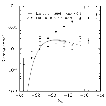
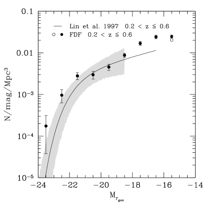
Figure 14: Left panel: Comparison of the R-band luminosity function of the FDF (filled/open circles, $\langle z\rangle\sim 0.3$) with the Schechter function derived in Lin et al. (1996) ($\langle z\rangle\sim 0.1$). The shaded region is based on $\Delta$M^∗, $\Delta\phi^{\ast}$, and $\Delta\alpha$. The triangles show the r’-band FDF LF at $\langle z\rangle\sim 0.3$ for SED type 1 galaxies. Right panel: Comparison of the Gunn-r-band LF of the FDF with the Schechter function derived in Lin et al. (1997) ($z=0.2$–$0.6$). The shaded region is based on $\Delta$M^∗, $\Delta\phi^{\ast}$, and $\Delta\alpha$.

Brown et al. (2001):
Brown et al. (2001) use 64 deg² of V and R images to measure the local V- and R-band LF. They analyzed about 1250 V & R selected galaxies from the Century Survey (Geller et al., 1997) with a mean spectroscopic redshift of $\langle z\rangle\sim 0.06$.
A comparison between the LF of Brown et al. (2001) and the FDF is shown in Fig. 15 for the V-band (left panel) and the R-band (right panel). Although the agreement is quite good for the bright end, the number density of the faint-end is substantially higher in the FDF (while the slope of the LF derived in the FDF is $\alpha=-1.25$, the slope derived by Brown et al. (2001) is $\alpha=-1.09\pm 0.09$ in the V- as well as in the R-band).

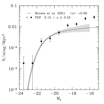
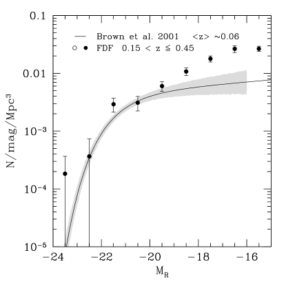
Figure 15: Comparison of the V-band (left panel) and R-band (right panel) LF of the FDF with the local ($\langle z\rangle\sim 0.06$) Schechter function derived in Brown et al. (2001). The shaded region is based on $\Delta$M^∗, $\Delta\phi^{\ast}$, and $\Delta\alpha$.

Shapley et al. (2001):
Shapley et al. (2001) analyzed 118 photometrically selected LBGs with K_s-band measurements covering an area of 30 arcmin². 63 galaxies have additional J-band measurements and 81 galaxies are spectroscopically confirmed. Using this sample Shapley et al. (2001) derived the luminosity function in the restframe V-band at redshift of $\langle z\rangle\sim 3.0$. Fig. 16 shows a comparison of the V-band LF derived by Shapley et al. (2001) with the LF in the FDF at $\langle z\rangle\sim 3.0$. The agreement is very good if we again concentrate on the shaded region. On the other hand, because of the depth of the FDF we can trace the LF two magnitudes deeper and therefore give better constraints on the slope of the Schechter function. Comparing the faint-end of the FDF LF with the extrapolated Schechter function of Shapley et al. (2001) clearly shows, that the very steep slope of $\alpha=-1.85$ is not seen in the FDF dataset.

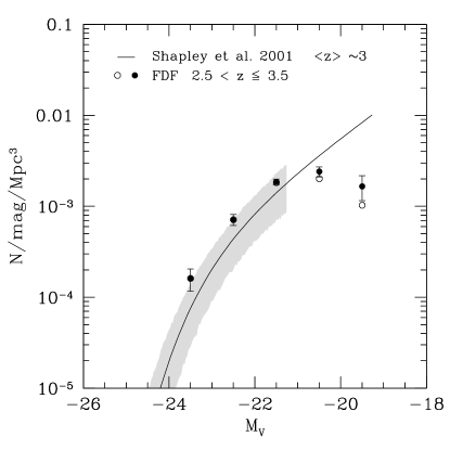
Figure 16: Comparison of the V-band luminosity function of the FDF with the Schechter function derived in Shapley et al. (2001) at $\langle z\rangle\sim 3.0$. The shaded region is based on $\Delta$M^∗, $\Delta\phi^{\ast}$, and $\Delta\alpha$, where the cut-off at low luminosity indicates the limiting magnitude of the sample.

Ilbert et al. (2004):
Ilbert et al. (2004) investigated the evolution of the galaxy LF from the VIMOS-VLT Deep Survey (VVDS) in 5 restframe bands (U, B, V, R, I). They used about 11000 objects with spectroscopic distance information in the magnitude range $17.5\leq I\leq 24.0$ to constrain the LF to redshift $z\sim 2$. In Fig. 17 we compare the V, R, and I band LF of the FDF with the Schechter function derived in the VVDS survey for different redshift bins: $0.20<z\leq 0.40$, $0.40<z\leq 0.60$, $0.60<z\leq 0.80$, $0.80<z\leq 1.00$, $1.00<z\leq 1.30$, and $1.30<z\leq 2.00$. Because of the limited sample size of the FDF at low redshift we could not use the same local redshift binning as Ilbert et al. (2004). We therefore compare in Fig. 17 (first row) the VVDS Schechter function at $\langle z\rangle\sim 0.3$ (light gray) and $\langle z\rangle\sim 0.5$ (dark gray) with the FDF LF derived at $0.2<z\leq 0.6$ as well as in Fig. 17 (second row) the Schechter function at $\langle z\rangle\sim 0.7$ (light gray) and $\langle z\rangle\sim 0.9$ (dark gray) with the FDF LF derived at $0.6<z\leq 1.0$. There is a very good agreement between the FDF data and the VVDS survey at all redshifts under investigation if we compare only the magnitude range in common to both surveys (shaded region). Ilbert et al. (2004) derived the faint-end slope from shallower data if compared with the FDF which have only a limited sensitivity for the latter. Nevertheless, in all three bands the differences between the formal $\alpha$ derived in the FDF ($\alpha_{V}=-1.25\pm 0.03$ and $\alpha_{r^{\prime}\&i^{\prime}}=-1.33\pm 0.03$ constant in redshift) and in the VVDS are compatible within $1\sigma$ to $2\sigma$ up to redshift $z\sim 0.8$ (only one bin in the I-band LF differs by slightly more than $2\sigma$). At higher redshift we do not see the steep slope ($\sim-1.5$) as derived by Ilbert et al. (2004). The circumstance that in the FDF we are able to follow the LF about 3 – 4 magnitudes deeper may explain the disagreement between the extrapolated faint-end slope of Ilbert et al. (2004) and the FDF result.

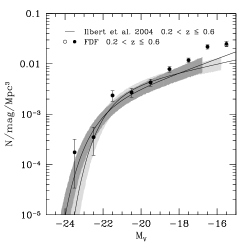
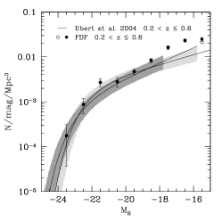
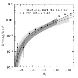
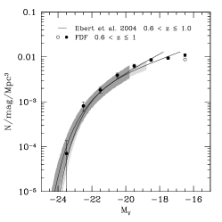
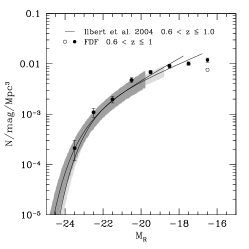
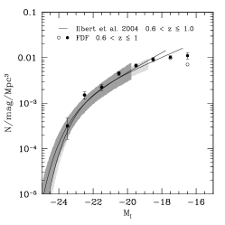
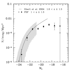
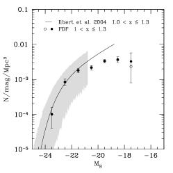
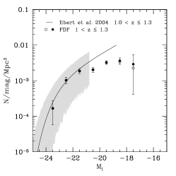
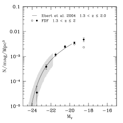
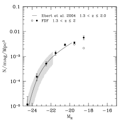
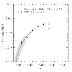
Figure 17: Comparison of the V (left panels), R (middle panels), and I (right panels) band LF of the FDF with the Schechter function derived in Ilbert et al. (2004) (VVDS) at $0.20<z\leq 0.40$ (first row, light gray), $0.40<z\leq 0.60$ (first row, dark gray), $0.60<z\leq 0.80$ (second row, light gray), $0.80<z\leq 1.00$ (second row, dark gray), $1.00<z\leq 1.30$ (third row), and $1.30<z\leq 2.00$ (fourth row). The shaded regions of all plots with $z\leq 1$ are based on $\Delta$M^∗, $\Delta\phi^{\ast}$, and $\Delta\alpha$. Only in the two high redshift bins (third and fourth row) the shaded region is based only on $\Delta$M^∗ and $\Delta\phi^{\ast}$. Please note that we use the average error if the upper and lower values reported by Ilbert et al. (2004) disagree.

Wolf et al. (2003):
In Fig. 18 we compare the r’-band LF of the FDF with the R-band selected luminosity function derived in the COMBO-17 survey (Wolf et al., 2003) for different redshift bins: 0.2 – 0.6, 0.6 – 0.8, 0.8 – 1.0, 1.0 – 1.2. Because of the limited sample size of the FDF at low redshift we could not use the same local redshift binning as Wolf et al. (2003). We compare therefore in Fig. 18 (upper left panel) the COMBO17 Schechter function at $\langle z\rangle\sim 0.3$ (light gray) and $\langle z\rangle\sim 0.5$ (dark gray) with the FDF LF derived at $0.2<z\leq 0.6$. There is a very good agreement between the FDF data and the COMBO-17 survey at all redshifts under investigations if we compare only the magnitude range in common to both surveys. Although the number density of the FDF seems to be slightly higher for the restframe UV LF (FDFLF I), this is not the case if we compare the LF in the R-band. Wolf et al. (2003) derived the faint-end slope from relatively shallow data which have only a limited sensitivity for the latter. This may explain the disagreement between the extrapolated faint-end slope of Wolf et al. (2003) and the FDF result.

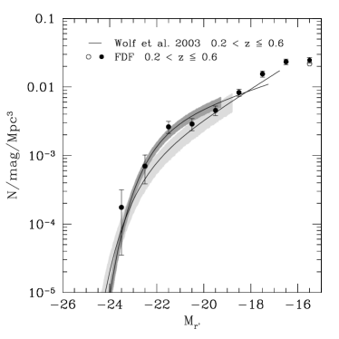
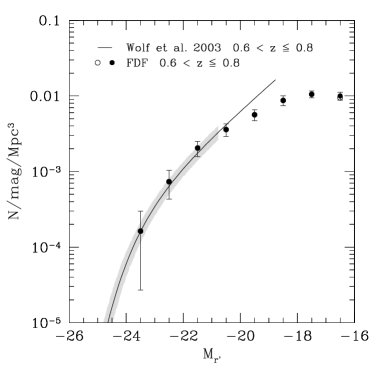
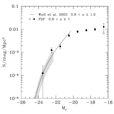
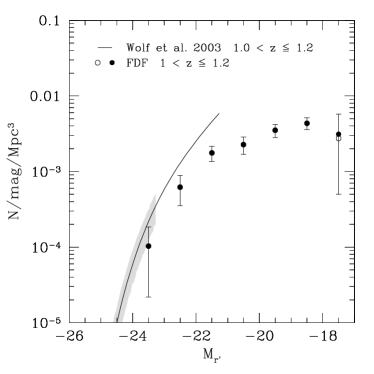
Figure 18: Comparison of the LF in the r’-band of the FDF with the Schechter function derived in Wolf et al. (2003): $0.2<z\leq 0.4$ (upper left panel, light gray), $0.4<z\leq 0.6$ (upper left panel, dark grey), $0.6<z\leq 0.8$ (upper right panel), $0.8<z\leq 1.0$ (lower left panel), $1.0<z\leq 1.2$ (lower right panel). The shaded regions of nearly all plots are based on $\Delta$M^∗, $\Delta\phi^{\ast}$, and $\Delta\alpha$. Only in the highest redshift bin (lower right panel) the shaded region is based only on $\Delta$M^∗ and $\Delta\phi^{\ast}$. The cut-off at low luminosity indicates the limiting magnitude of the sample.

Chen et al. (2003):
The galaxy sample analyzed by Chen et al. (2003) contains $\sim 6700$ H-band selected galaxies (within 847 arcmin²) in the HDFS region with complementary optical U, B, V, R, and I colors, and $\sim 7400$ H-band selected galaxies (within 561 arcmin²) in the Chandra Deep Field South region with complementary optical V, R, I, and z’ colors. The galaxy sample is part of the Las Campanas Infrared Survey (LCIR Marzke et al., 1999; McCarthy et al., 2001) and based on photometric redshifts.

Fig. 19 shows a comparison of the R-band luminosity function derived by Chen et al. (2003) with the LF in the FDF for three different redshift bins: 0.50–0.75 (left panel), 0.75–1.00 (middle panel), and 1.00–1.50 (right panel). There is a good agreement between the FDF LF and the Schechter function derived by Chen et al. (2003) in the lowest redshift bin ($z=0.50$–$0.75$) if we compare only the magnitude range in common to both surveys. At intermediate redshift ($z=0.75$–$1.00$) the number density of the bright end of the FDF LF is slightly higher than in Chen et al. (2003). On the other hand, for the highest redshift bin ($z=1.00$–$1.50$) the number density of the bright end derived by Chen et al. (2003) roughly agrees with the results obtained in the FDF.

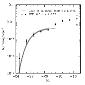
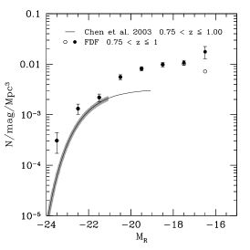
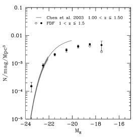
Figure 19: Comparison of the luminosity function in the R-band of the FDF with the Schechter function derived in Chen et al. (2003): $0.50<z\leq 0.75$ (left panel), $0.75<z\leq 1.00$ (middle panel), and $1.00<z\leq 1.50$ (right panel). The shaded region is based on $\Delta$M^∗, $\Delta\phi^{\ast}$ and $\Delta\alpha$ for $0.50<z\leq 0.75$ (left panel). For $0.75<z\leq 1.00$ (middle panel) and $1.00<z\leq 1.50$ (right panel) the shaded region is based only on $\Delta$M^∗ and $\Delta\phi^{\ast}$. The cut-off at low luminosity indicates the limiting magnitude of the sample.

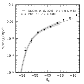
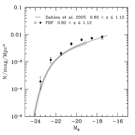
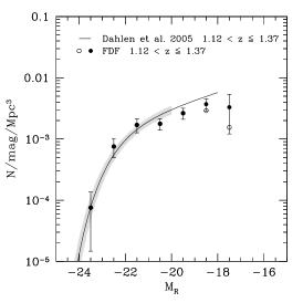
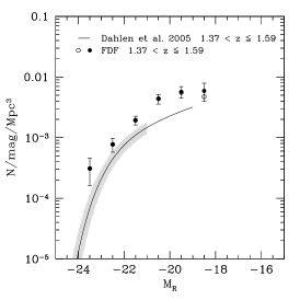
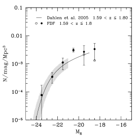
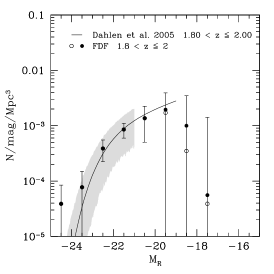
Figure 20: Comparison of the R-band LF of the FDF with the Schechter function derived in Dahlen et al. (2005) at $0.10<z\leq 0.82$, $0.82<z\leq 1.12$, $1.12<z\leq 1.37$, $1.37<z\leq 1.59$, $1.59<z\leq 1.80$, and $1.80<z\leq 2.00$ (from upper left to lower right panel). The shaded region is based on $\Delta$M^∗, $\Delta\phi^{\ast}$ and $\Delta\alpha$ for all panels. The cut-off of the shaded region at low luminosity indicates the limiting magnitude of the sample.

Dahlen et al. (2005):
Dahlen et al. (2005) used HST and ground-based $U$ through $K_{s}$ photometry in the GOODS-S Field to measure the evolution of the R-Band luminosity function out to $z\sim 2$. They combine a wider area ($\sim 1100$ arcmin²), optically selected ($R<24.5$) catalog with a smaller area ($\sim 130$ arcmin²) but deep NIR selected ($K_{s}<23.2$) catalog. Distances are based on photometric redshifts with an accuracy of $\Delta z/(z_{spec}+1)\sim 0.12$ ($\sim 0.06$ after excluding $\sim$ 3% of outliers). To determine the restframe R-band galaxy luminosity function out to $z\sim 2$ they used the deep $K_{s}$ selected catalog. A comparison between the R-band LF of Dahlen et al. (2005) and the FDF is shown in Fig. 20. There is a very good agreement in nearly all redshift bins. Only at $0.82<z\leq 1.12$ and $1.37<z\leq 1.59$ the characteristic density in the FDF seems to be slightly higher.

To summarize we can say, that the LFs derived in the FDF in general show a very good agreement with other observational datasets from the literature. At the bright end of the LF most of the datasets agree within $1\sigma$. Differences between the extrapolated Schechter function of the literature and the measured faint-end in the FDF can be attributed to the shallower limiting magnitudes of the other surveys.

5 Comparison with model predictions

Figure 21: Comparison of the R-band LF of the FDF with predictions based on Kauffmann et al. (1999) (solid line): $\langle z\rangle\sim 0.20$, $\langle z\rangle\sim 0.62$, and $\langle z\rangle\sim 1.05$, (from left to right panel). The filled (open) symbols show the LF corrected (uncorrected) for $V/V_{max}$. The drops of the theoretical curves towards the faint-end is caused by the limited mass resolution of the models, see Kauffmann et al. (1999) for details.

Figure 22: Comparison of the I-band LF of the FDF with predictions based on Kauffmann et al. (1999) (solid line): $\langle z\rangle\sim 0.20$, $\langle z\rangle\sim 0.62$, $\langle z\rangle\sim 1.05$, $\langle z\rangle\sim 1.46$, $\langle z\rangle\sim 2.12$, and $\langle z\rangle\sim 2.97$ (from upper left to lower right panel). The filled (open) symbols show the LF corrected (uncorrected) for $V/V_{max}$. The drops of the theoretical curves towards the faint-end is caused by the limited mass resolution of the models, see Kauffmann et al. (1999) for details.

As discussed for example in Benson et al. (2003) different physical processes are involved in shaping the bright and the faint-end of the galaxy LF. Therefore, it is interesting to compare LFs predicted by models with observational results to better constrain those processes. In this section we compare the R-band and I-band LFs in different redshift bins with model predictions of Kauffmann et al. (1999).
In Fig. 21 we show the R-band luminosity function of the FDF together with the semi-analytic model predictions by Kauffmann et al. (1999) for $\langle z\rangle\sim 0.20$, $\langle z\rangle\sim 0.62$, $\langle z\rangle\sim 1.05$, whereas in Fig. 22 we show the I-band LF in the redshift bins $\langle z\rangle\sim 0.20$, $\langle z\rangle\sim 0.62$, $\langle z\rangle\sim 1.05$, $\langle z\rangle\sim 1.46$, $\langle z\rangle\sim 2.12$, and $\langle z\rangle\sim 2.97$. For the R-band no semi-analytic model predictions are available for redshifts larger than $\langle z\rangle\sim 1.05$.
There is a good agreement between model (solid lines) and measured LFs in the R-band. Also for the I-band there is a good agreement between the models and the luminosity functions derived in the FDF up to redshift $\langle z\rangle\sim 1.46$ (of course at $z\approx 0$ the model is tuned to reproduce the data). At $\langle z\rangle>1.46$ the discrepancy increases as the model does not contain enough bright galaxies. Unfortunately, the models only predict luminosities for massive galaxies and because of lack of resolution do not predict galaxy number densities for faint galaxies.

6 Summary and conclusions

In this paper we use a sample of about 5600 I-band selected galaxies in the FORS Deep Field down to a limiting magnitude of I $=26.8$ mag to analyze the evolution of the LFs in the r’, i’, and z’ bands over the redshift range $0.5<z<3.5$, thus extending the results presented in FDFLF I to longer wavelengths. All the results are based on the same catalog and the same state of the art photometric redshifts ($\Delta z/(z_{spec}+1)\leq 0.03$ with only $\sim 1$% outliers) as in FDFLF I. The error budget of the luminosity functions includes the photometric redshift error of each single galaxy as well as the Poissonian error.
Because of the depth of the FDF we can trace the LFs deeper than most other surveys and therefore obtain good constraints on the faint-end slope $\alpha$ of the LF. A detailed analysis of $\alpha$ leads to similar conclusions as found in FDFLF I for the blue regime: the faint-end of the red LFs does not show a large redshift evolution over the redshift range $0.5\mathrel{\hbox to0.0pt{\lower 4.0pt\hbox{\hskip 1.0pt$\sim$}\hss}\raise 1.0pt\hbox{$<$}}z\mathrel{\hbox to0.0pt{\lower 4.0pt\hbox{\hskip 1.0pt$\sim$}\hss}\raise 1.0pt\hbox{$<$}}2.0$ and is compatible within $1\sigma$ to $2\sigma$ with a constant slope in most of the redshift bins. Moreover, the slopes in r’, i’, and z’ are very similar with a best fitting slope of $\alpha=-1.33\pm 0.03$ for the combined bands and redshift intervals considered here.
Interestingly, an analysis of the slope of the LFs as a function of wavelength shows a prominent trend of $\alpha$ to steepen with increasing wavelength: $\alpha_{UV\&u^{\prime}}=-1.07\pm 0.04$ $\rightarrow$ $\alpha_{g^{\prime}\&B}=-1.25\pm 0.03$ $\rightarrow$ $\alpha_{r^{\prime}\&i^{\prime}\&z^{\prime}}=-1.33\pm 0.03$. To better understand this wavelength-dependence of the LF slope, we analyze the contribution of different galaxy types to the overall LF by subdividing our galaxy sample into 4 typical SED types with restframe U-V colors between 2.3 – 1.9, 2.0 – 1.6, 1.6 – 0.9, and 0.9 – 0 for SED type 1, 2, 3, and 4, respectively. Therefore, in a rough classification one can refer to SED types 1 and 2 (SED type 3 and 4) as red (blue) galaxies.
Although in the UV regime the overall LF is completely dominated by extremely star-forming galaxies, the overall LF in the red regime is mainly dominated by early to late type galaxies at the bright end, but extremely star-forming galaxies at the faint-end. The relative contribution of the different SED type LF to the overall LF clearly changes as a function of analyzed waveband resulting (at the depth of the FDF) in a steeper slope for the overall LF in the red regime if compared to the blue regime.
To quantify the contribution of the different SED types to the total luminosity density, we derive and analyze the latter in the UV and in the red bands as a function of redshift: The contribution of type 1 and 2 galaxies to the UV LD is negligible at all analyzed redshifts as SED type 3 and 4 completely dominate. On the other hand, the relative contribution to the overall luminosity density of type 1 and 2 galaxies is of the same order or even exceeds those of type 3 and 4 in the red bands.

We investigate the evolution of M^∗ and $\phi^{\ast}$ (for a fixed slope $\alpha$) by means of the redshift parametrization introduced in FDFLF I. Based on the FDF data (Case 1 and Case 2), we find only a mild brightening of M^∗ and decrease of $\phi^{\ast}$ with increasing redshifts in all three analyzed wavebands. If we follow the evolution of the characteristic luminosity from $\langle z\rangle\sim 0.5$ to $\langle z\rangle\sim 3$, we find an increase of $\sim$ 0.8 magnitudes in the r’, and $\sim$ 0.4 magnitudes in the i’ and z’ bands. Simultaneously the characteristic density decreases by about 40 % in all analyzed wavebands. We compare the LFs with previous observational datasets and discuss discrepancies. As for the blue bands, we find good/very good agreement with most of the datasets especially at the bright end. Differences in the faint-end slope in most cases can be attributed to the shallower limiting magnitudes of the other surveys.

We also compare our results with predictions of semi-analytical models at various redshifts. The semi-analytical models predict LFs which describe the data at low redshift very well, but as for the blue bands, they show growing disagreement with increasing redshifts. Unfortunately, the models only predict luminosities for massive galaxies and therefore, a comparison between the predicted and observed galaxy number densities for low luminosity galaxies ($L\mathrel{\hbox to0.0pt{\lower 4.0pt\hbox{\hskip 1.0pt$\sim$}\hss}\raise 1.0pt\hbox{$<$}}L^{\ast}$) could not be done.