Halos of Spiral Galaxies. I. The Tip of the Red Giant Branch as a Distance Indicator

Abstract

We have imaged the halo populations of a sample of nearby spiral galaxies using the Wide Field Planetary Camera 2 on broad the Hubble Space Telescope with the aim of studying the stellar population properties and relating them to those of the host galaxies. In four galaxies, the red-giant branch is sufficiently well populated to measure the magnitude of the tip of the red-giant branch (TRGB), a well-known distance indicator. Using both the Sobel edge-detection technique and maximum-likelihood analysis to measure the $I$-band magnitude of the red giant branch tip, we determine distances to four nearby galaxies: NGC 253, NGC 4244, and NGC 4945, NGC 4258. For the first three galaxies, the TRGB distance determined here is more direct, and likely to be more accurate, than previous distance estimates. In the case of NGC 4258, our TRGB distance is in good agreement with the the geometrical maser distance, supporting the the Large Magellanic Cloud distance modulus $(m-M)_{0}=18.50$ that is generally adopted in recent estimates of the Hubble constant.

1 Introduction

1.1 Spiral galaxy Halos

The diffuse stellar halo component of galaxies represents a tiny fraction of the mass (about 1% in the case of the Milky Way; Morrison 1993) and the low surface brightness of the population makes study in extragalactic settings difficult. However, galactic halos are unique laboratories for investigating fundamental galaxy properties. Age and/or metallicity distributions of halo stellar populations and their kinematics provide fossilized glimpses of the earliest conditions of galaxy formation. Halo populations may give us answers to key questions about the chronology of galaxy formation: how the halo formation was related to the assembly of galactic mass and the formation of galaxies.

Different views have been advanced toward understanding the formation of galactic stellar halos. The first scenario was proposed by Eggen, Lynden-Bell, & Sandage (1962), where the authors proposed that the metal-poor stars in the Galactic halo were formed during a rapid collapse of a relatively uniform, isolated protogalactic cloud. This picture is generally viewed as advocating a rapid dissipative and monolithic collapse of protogalaxies.

An increasing number of observational findings, both at high redshift and in nearby galaxies, together with cosmological models of structure formation, challenge this general view, and suggest an alternative picture of how halos of galaxies may have formed. This alternative paradigm for halo formation is based on the idea that the galactic halo was formed via the accretion, over an extended period, of small metal-poor satellites which underwent independent chemical evolution before being accreted (Searle & Zinn 1978; see also Freeman 1987). The disruption of globular clusters, revealed by tidal tails (Grillmair et al. 1995), may also contribute to the stellar halo (Aguilar et al. 1988). This is supported by the observation that halo field stars and globular clusters in the Milky Way have similar mean metallicities (Carney 1993). Note that this is not the case for M 31 stellar halo (Durrell et al. 2001, Perrett et al. 2002). An interesting consequence of this hypothesis is that a fraction of globular clusters may be stripped relics of highly nucleated dwarf satellites (see Freeman & Bland-Hawthorn 2002 for a detailed discussion). The discovery of the Sgr dwarf galaxy (Ibata et al. 1994), streams and moving groups in halos of both the Galaxy (Yanny et al. 2000; Ivezic et al. 2000; Dohm-Palmer et al. 2001) and M31 (Ibata et al. 2001) encourage renewed interest in halo formation through accretion of smaller protogalactic structures.

Although great effort has been dedicated in recent years to investigate stellar populations and/or kinematic of Local Group spiral halos, it is unlikely that the problem of galactic halo formation may be understood entirely by studies of these galaxies alone. Questions about the universality of halo formation mechanism(s), the similarity of halo global properties and their sensitivity to disk and/or bulge properties, among others, will require a larger sample of galaxies.

One means of addressing these questions is to extend the study of galaxy halos to other spiral galaxies. Such studies are now within reach of the HST. Our purpose is to study systematically the global properties of population II halos of nearby normal spiral galaxies. Such a program may reveal whether there was a universal formation mechanism, or whether there are mixture of different stellar halos; if the halos are dominated by formation of the nuclear bulge and perhaps enriched by gas outflow, or composed of debris of disintegrated dwarf galaxies revealed by the presence of a large fraction of intermediate age stellar populations. Also of great interest is the investigation of whether halo and disk/bulge properties are correlated.

In order to interpret the color-magnitude diagrams (CMDs) of resolved stars in nearby galaxies it is important to have reliable distance estimates. Fortunately, sometimes the CMDs themselves provide such an estimate.

1.2 A distance indicator to nearby galaxies: the tip of the red giant branch

Stars on the first-ascent red giant branch (RGB) climb this phase with an expanding convective envelope and an hydrogen burning shell. While evolving through the RGB, low-mass stars develop an electron-degenerate core, which causes an explosive start of the core-He burning phase, the so-called He-flash, almost independently from the initial stellar parameters, such as initial mass or abundance (Chiosi et al. 1992). The He-flash is followed by a sudden decrease of the stellar luminosity due to the extinction of the H-burning shell. Hence low-mass stars will accumulate along the RGB, reaching their maximum luminosity, during this phase, at the tip of RGB (TRGB). This behavior translates to an abrupt discontinuity in the luminosity function (Renzini 1992). As the evolution of the RGB stars depends essentially on the core-mass, the number of stars per luminosity interval will be related directly to the He-core growth rate (Iben & Renzini 1983). Theoretical and observational investigations find the luminosity function of RGB stars to follow a simple power-law (see Zoccali & Piotto 2000 and references therein). The TRGB magnitude is the location where the RGB luminosity function truncates. Below metallicities ${\rm[Fe/H]\approx-0.7}$, the location of the TRGB in the $I$ band is expected to be quite insensitive to age and/or metallicity (e.g., Salaris & Cassisi 1997). At higher metallicities, bolometric corrections in the $I$ band become important and the TRGB magnitude becomes increasingly sensitive to metallicity (e.g., Salaris & Girardi 2005).

The TRGB method is also well supported observationally. The location of the absolute I-band TRGB luminosity for a sample of Galactic globular clusters spanning a large range of abundances, ${\rm-2.1\leq[\rm Fe/H]\leq-0.7}$, over ages spanning 2-15 Gyr (Da Costa & Armandroff 1990), is quite stable and insensitive to age and metallicity (for $[\rm Fe/H]\leq-0.7$), changing by less than $\sim\,0.1\,$mag (Lee et al. 1993).

Good agreement is generally found between the distances obtained using the TRGB method and classical distance indicators such as Cepheid and RR Lyrae variables (e.g., Sakai et al. 1996, Ferrarese et al. 2000). Being a population II distance indicator, unlike the Cepheid method (population I distance indicator), the TRGB method can be applied to any class of galaxies, making this an attractive and easy technique to use to estimate galaxy distances.

Because the outer regions of galaxies are devoid of significant concentrations of gas and dust and the stellar density is low, studies of standard candles in the halo provide a means of estimating distances free of assumptions concerning internal reddening in galaxies or crowding. In § 2, the details of observations using the HST Wide Field Planetary Camera 2 (WFPC2) and data reduction are reported. In § 3, we present the detection of RGB stars and the methods for measuring the TRGB using the $I$-band luminosity function that we have employed. Finally, in § 4, we present the color–magnitude diagrams, luminosity functions, and derived distances for the galaxies studied.

2 Data

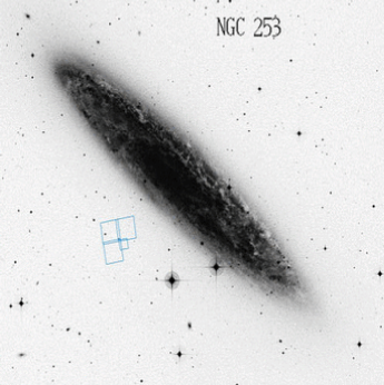
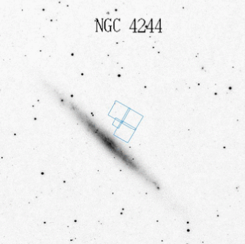
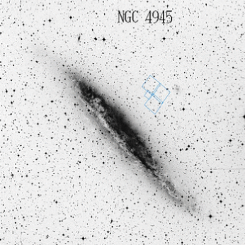
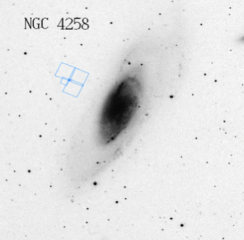
Figure 1: Locations of the observed halo fields being studied in the paper.

Until recently, no spiral galaxy halo outside of the Local Group had been imaged to a depth sufficient to permit study of the halo metallicity distribution function or other stellar population studies, such as the presence of intermediate-age stars. HST observations have begun to change this. We have observed a sample of spiral galaxies with the aim of unambiguously resolving their stellar halos down to one or two magnitudes below the TRGB. Our selection criteria of the sample galaxies are as follows. We seek spiral galaxies with (i) morphological types between Sa to Sc, (ii) distance moduli $(m-M)_{o}<29.5$, (iii) high inclinations, i.e., $i>45$ degrees, to reduce any contamination from the outer disk stars, and (iv) absolute magnitudes $M_{B}<-18$. The resulting sample of eight galaxies represents most of the nearby luminous inclined spiral galaxies. In this paper, we estimate the distances to four galaxies in our sample, i.e., NGC 253, NGC 4244, NGC 4258, and NGC 4945, using the tip of the red giant branch technique. Fig. 1 shows the locations of the observed halo fields, superimposed on the Digitized Sky Survey images of these galaxies. Madore & Freedman (1995) argue that in order to minimize potential biases and to securely identify the TRGB, there should be at least 50–100 stars in the first magnitude interval of the RGB star luminosity function. With sparser data sets the distance modulus tends to be overestimated. Four galaxies in our sample have luminosity functions that are too poorly populated to yield reliable TRGB distances: NGC 55, NGC 247, NGC 300, and NGC 3031. Hence these galaxies are not discussed in the present paper; the color-magnitude diagrams of the observed halo fields for these galaxies are shown and discussed in paper III of this series. Tikhonov, Galazutdinova & Drozdovsky (2005) estimate TRGB distances for three of these galaxies using larger HST data sets.

The galaxy sample is summarized in Table 1. The galaxies were observed through the F814W and F606W filters. Exposure times through the F814W filter were set to reach S/N = 5 in the WF camera for an absolute magnitude ${\rm M_{I}=-1}$ (for galaxies with $(m-M)_{0}<27$) or ${\rm M_{I}=-2}$ (for NGC4258 and NGC4945, which are more distant). The F606W exposure times were set to reach the same S/N at the same absolute magnitude for metal-poor RGB stars. The exposures were typically dithered over 3 separate pointings (the range being from 2 to 6) with a pattern extending over approximately 0.25 arcseconds to allow rejection of hot pixels and detector artifacts.

The images were reduced through the standard HST pipeline, using the latest flatfield observations and using contemporaneous super-dark reference frames. The dithered frames were combined with iterative cosmic ray rejection using software in the stsdas.dither package based on the drizzle algorithm of Fruchter and Hook (2002). Briefly, the images were drizzled (shifted, geometrically corrected, and resampled) to a common frame to construct a median image reasonably free of cosmic rays. This image was geometrically transformed back to the pixel grids of the original image and used as the truth image for identifying cosmic rays. The images were then re-drizzled onto a pixel scale of 0.1^′′, masking out the cosmic rays, hot pixels, and detector artifacts, using optimal weights based on the counts at the sky level in each image. A value pixfrac=0.8 was used to minimize the degradation of the image quality due to the resampling.

The stellar magnitudes were measured through circular apertures with a radius of 0.15″. These aperture magnitudes were corrected to total magnitudes using TinyTim model (Krist 2004) point-spread functions. Aperture-corrections and zeropoints are applied separately for each CCD chip. Magnitudes are in the Vega system (i.e., Vega has magnitude=0 through both filters, when measured through a 3″aperture). Diffuse sources have been excluded from the catalogs based on the magnitude difference between measurements through 0.09″and 0.3″apertures. Objects where this difference is greater than 1.3 magnitudes are generally galaxies or blends of stars. This demarcation was determined by starting with a Tiny-Tim prediction of the ratio of fluxes for a point source measured in those apertures. We mark objects in the images whose flux growth exceeds that prediction and iterate to arrive at a value which preserves point sources while excluding those with extended radial profiles.

The stellar photometry was corrected for charge-transfer efficiency (CTE hereafter) effects using the 31 May 2002 version of the Dolphin (2000) equations. The CTE correction amounts to a maximum of $\sim 0.2$ mag for faint stars at the top of the chip in fields with the highest background, such as NGC3031, while reaching $\sim 0.5$ mag in fields with low sky background, such as NGC55. Typically the maximum correction for the data is $-0.5$ mag.

Transformation of the instrumental magnitudes to standard V and I magnitudes followed the prescriptions of Holtzman et al. (1995). First, we have corrected from the foreground extinction using ${\rm A_{606W}=2.677\times E(B-V)}$ and ${\rm A_{814W}=1.815\times E(B-V)}$, then given the instrumental magnitudes, we have determined the standard Johnson-Cousins magnitudes by solving iteratively the second degree equations relating the WFPC2-to-VI magnitudes using the coefficients tabulated by Holtzman et al. (1995). Fig. 2 shows the evolution of the resulting photometric errors for I-band as a function of the apparent magnitude. The typical trend of increasing photometric errors with apparent magnitude can be seen, where most of the stars observed in the fields are affected by photometric errors of a few tenths of a magnitude.

3 Measuring the TRGB

To avoid stellar populations that may bias the analysis of the luminosity function, we have restricted our analysis to stars that match the location of the RGB sequence of metal-poor stellar populations. To do so, we have retained only stars that are bluer than a certain cut. For all the galaxies discussed in this paper, the remaining number of red giant stars after the color cut is sufficient for a reliable TRGB estimate by the criterion of Madore & Freedman (1995); i.e., there are more than 100 stars in the one-magnitude interval fainter than the TRGB. It is worth mentioning that as long as the aim is measurement of the TRGB, there is no need to include all the observed stars to construct the luminosity function. When the red giant branch is not well populated, metal-rich stars, i.e., ${\rm[Fe/H]\gtrsim-0.5}$, that occupy the red part of the CMD where no calibration is available, might make the tip of the red giant branch less well identifiable. Our simple color cut accomplishes this goal, but will lead to different overall luminosity functions for different metallicity distributions. This is not a problem, provided that the TRGB feature itself is clearly visible. The mean metallicities of halo stellar populations of all our sample galaxies are at or below ${\rm[Fe/H]\lesssim\,-0.6}$ (see the second paper of this series for more details), so any contamination from metal-rich stars is expected to be small.

We used two different methods to detect and to measure the TRGB I-band magnitude from the luminosity function of a stellar population. In the following subsections we present briefly our methodology.

3.1 Edge Detection

The most widely used procedure to estimate the TRGB I-band magnitude uses the abrupt termination of the RGB luminosity function at the TRGB magnitude. The TRGB discontinuity causes a peak in the first derivative of the observed stellar magnitude distribution (Lee et al. 1993; Madore & Freedman 1995). Sakai et al. (1996) update this method by Gaussian-smoothing the luminosity function to avoid the arbitrary choice of the binning size, and use a continuous edge detection function.

Due to the power-law form of the RGB luminosity function, we use a kernel-smoothed logarithmic luminosity distribution function filtered by a Sobel kernel to determine the luminosity of the TRGB; the edge detection function is:

$$E(m)\,=\,\log_{10}(\Phi(m+\sigma_{m}))-\log_{10}(\Phi(m-\sigma_{m})).$$ (1)

where $\sigma_{m}$ is the photometric error, estimated as the mean of photometric errors shown in Fig. 2, within a bin of $\pm 0.05$ magnitude about a magnitude $m$ (Sakai et al. 1996). The edge detection filter essentially measures the slope of the luminosity function, and hence it is very sensitive to the noise; any sudden change in the signal is extremely amplified by the filtering scheme. To suppress any detection of statistically non-significant peaks in the first derivative of the luminosity function, we apply a weighting scheme to the edge detection filtering output (Sakai et al. 1997; Mendez et al. 2002). Each $E(m)$ is weighted by the Poisson noise (i.e.,$\Phi(m)^{1/2}$).

Cioni et al. (2000) have found the edge detection technique to be a biased estimator of the TRGB magnitude. However, the bias depends on the photometric errors and the amount of smoothing in the luminosity function at the location of the TRGB. For our data set, the bias is less than $0.03-0.04$ magnitude (Cioni et al. 2000), much smaller than the random errors; therefore the distance modulus to the galaxy sample we derive using the edge detection technique would not be significantly affected in a comparison with the maximum likelihood (see below).

To estimate the statistical uncertainty in measuring the $I$-band TRGB magnitude, we use bootstrap resampling of the data to generate a large number of samples drawn from the original data set to simulate the act of observing multiple times. Using this procedure to quantify the formal errors in measuring the TRGB has the advantage of using the empirical distribution function derived from the data itself, rather than a particular functional form (e.g., Gaussian) for the photometric errors.

For each galaxy in our sample, we perform the bootstrap resampling and calculate the statistic of interest $N\sim\,n\times\,[\log(n)]^{2}$ times, where $n$ is the number of observed stars within the magnitude range where the luminosity function model is valid in the case of maximum likelihood analysis, and the number of stars used to construct the luminosity function in the case of Sobel edge detection analysis. To this extent the bootstrap version of a statistic’s sampling distribution matches the asymptotic sampling distribution (see Babu & Feigelson 1996 and Efron & Tibshirani 1986 for reviews of the theory and application of this technique). In these bootstrap samples, the standard deviation of the I-band TRGB distribution is taken as the random error in the measurement of the TRGB magnitude. This procedure allows a more robust estimate of the statistical errors than using the full-width at half maximum of the observed peak in the first luminosity function derivative, as usually done (Sakai et al. 1996; see also Mendez et al. 2002 and Cioni et al. 2001).

3.2 Maximum Likelihood Analysis

An alternative to filtering is to fit models to the data using the technique of maximum likelihood; this avoids concerns over binning and kernel smoothing. While theory does not provide strong guidance on the exact functional form of the luminosity function near the TRGB, a simple two-power-law model appears to provide a good empirical fit over a restricted range of magnitudes near the TRGB itself. The TRGB itself is identified as the break between the two power laws.

In this technique, the underlying luminosity function is treated as a probability distribution function (PDF) and we compare relative likelihoods of drawing the observed data set from the model PDFs as we vary the model parameters. An advantage of this procedure is that no data binning is needed. In practice we have binned the both the probability distributions and the data in intervals of 0.002 mag, as it simplifies the fitting procedure.

Given a model of the stellar distribution on the RGB, $\Phi(m|{\bf\theta})$k, where $\theta$ is the set of free parameters characterizing the model, the likelihood that the observed data set is drawn from this model is given simply by the product of individual probabilities that star $i$ has an observed magnitude $m_{i}$ within a range $dm$:

$${\cal L(\theta)}=\prod_{i}P_{i}({\bf\theta})\propto\prod_{i}\Phi(m_{i}|{\bf\theta})$$ (2)

where $P_{i}$ is the individual probability defined as the ratio of the number of stars actually observed at a given magnitude by the total number of stars expected given a luminosity function model $\Phi(m|{\bf\theta})$.

Photometric errors will affect the magnitude distribution of the observed stars. To account for this, we convolve the intrinsic luminosity function models with an appropriate broadening function, $\Sigma(m)$, to obtain the distribution of observed magnitudes. This function describes the probability that a star with an intrinsic magnitude $m_{int}$ is observed to have the magnitude $m_{obs}=m_{int}+m$. Thus the distribution of the observed magnitudes is:

$$\Phi(m_{i})=\int g(m|\theta)\Sigma(m_{i},m)dm$$ (3)

where $g(m|\theta)$ is the intrinsic luminosity function model.

We represent the measurement error by a Gaussian function with a total dispersion $\sigma_{m}$. That is, we have

$$\Sigma(m_{i},m)\,=\,\frac{1}{(2\pi)^{1/2}\,\sigma_{m_{i}}}\exp\left[-\frac{(m-m_{i})^{2}}{2\sigma_{m_{i}}^{2}}\right]$$ (4)

where $\sigma_{m_{i}}$ is the photometric error at the magnitude $m_{i}$. The probability of observing a star of a magnitude $m_{i}$ in a magnitude range $dm$ is simply $g(m_{i}|\theta)\,dm$. The photometric errors smear the probability to the shape of the error function, centered at $m_{i}$; then the probability becomes $\Sigma(m_{i},m)\,g(m_{i}|\theta)\,dm$. The photometric errors were determined from artificial star tests. We take the output of these simulations in 0.5 mag intervals for input stars of a fixed color V-I = 1.0. In each 0.5 mag interval, we determine the mean and standard deviation of the residuals of recovered minus input I-band magnitudes. For smearing the model luminosity functions, we use a set of Gaussian kernels with the mean and standard deviation that were determined from the simulations and with an overall normalization set by the fractional completeness in that 0.5 mag interval. The model luminosity functions are convolved with these kernels prior to estimating the logarithm of the likelihood.

The maximum likelihood fitting is restricted to the magnitude range where the effects of both the photometric errors and the incompleteness are not large. To avoid contamination from metal-rich stars that may bias the estimate of the TRGB location, we consider only blue stars, i.e., stars within the color range ${\rm-2<(V-I)<2}$ (in practice there are few stars bluer than $V-I=0.5$). Ideally, it would be best to fit a curved TRGB to a locus of RGB models of all metallicities. However, in practice the resolution of existing isochrones near the TRGB is insufficient for this purpose, and also the isochrones themselves have been constructed via a series of interpolations that become increasingly uncertain near the TRGB. For this reason, the TRGB distance indicator remains an empirical test: a search for a clear jump or inflection in the luminosity function.

To approximate the intrinsic luminosity function $g(m|\theta)$, we use a broken power-law model (Cioni et al. 2000; Mendez et al. 2002; Gregg et al. 2004). The free parameters characterizing the intrinsic model are the logarithm of the amplitude of the discontinuity at the TRGB, the apparent magnitude of the TRGB break, and the slopes of luminosity function on either side of the break.

We used both the Nelder-Mead (1965) simplex algorithm and “simulated annealing” (e.g., Metropolis, 1953; Press et al. 1992) to determine the best-fit model. Results of the two methods were similar, and well within the uncertainties derived from the subsequent error analysis.

To determine the uncertainties in the TRGB magnitude, we have stochastically sampled the full model parameter space by building a Monte-Carlo Markov Chain (MCMC) using the Metropolis-Hastings update mechanism. There is a growing body of literature on this technique (e.g., Knox, Christensen & Skordkis 2001; Verde et al. 2003), which provides an efficient way to characterize the likelihood manifolds in a multi-dimensional parameter space. The Metropolis-Hastings MCMC algorithm is a restricted random walk through parameter space. At each step in the random walk, magnitude and direction of the next step is drawn from a normalized “proposal density” $q(y,x)$, where the new state $y$ depends only on the current state $x$. The candidate $y$ is accepted or rejected with a probability

$${\rm min}\left(1,\frac{p(y)}{p(x)}\frac{q(y,x)}{q(x,y)}\right),$$ (5)

where $p(y)/p(x)$ is the likelihood ratio for state $x$ relative to state $y$. After a period of “burn-in,” the distribution of locations in parameter space sampled by the chain converges to the “posterior distribution” $p$. Thus likelihood contours can be constructed simply by drawing contours of the density of points sampled by the chain.

For our proposal distribution, we have used a Gaussian with $\sigma=0.1$ in all of the fit parameters. We have also restricted the chains to operate within a “reasonable” range of parameter space: break amplitudes within a factor of 100 of the best fit, TRGB magnitudes within 1.5-2 mag of the best fit, and LF slopes between $-5$ and $+0.2$. The chains were burned in for 1000 steps, and then 10000 steps were used to sample the posterior distributions. The probability distributions thus derived are shown in the lower-right panels of Figures 3-6. We have verified that the results are insensitive to small changes in the range of magnitudes being fit and the parameters used to define the MCMC. The confidence intervals (and indeed the best fit values) are nevertheless subject to a number of implicit prior assumptions. These include the assumption that the distribution can be adequately described by two power laws with a break, over the full magnitude range being fit. In practice, we do see small but significant differences in the confidence intervals as we change the magnitude limits and color limits. However shifts of 0.2 mag in these limits in all of our tests shift the peak of the likelihood distribution by less than the $1\sigma$ widths show in Figs. 3-7.

4 TRGB Distances

As a first step to investigate the properties of field stellar populations in spiral galaxy halos, we have determined distances to a sample of galaxies. A summary of TRGB distances and uncertainties is presented in Table 1. Color-magnitude diagrams, luminosity functions, and other properties for our galaxy sample are presented in the next subsections. The best fitting luminosity function model, $\Phi(m|{\bf\hat{\theta}})$, where $\hat{\theta}$ is the free parameter set that maximize the likelihood, is overplotted on the observed luminosity function for each galaxy. Note that the smoothing by the photometric errors, accounted for in the maximum likelihood analysis, converts the abrupt break at the TRGB magnitude into a continuous RGB star distribution near the TRGB.

Once the I-band magnitude of the TRGB is measured, we use the semi-empirical calibration given by Lee et al. (1993) to determine the distance modulus, starting from the relation:

$$(m-M)_{I,o}\,=\,I_{TRGB}-M_{bol,TRGB}+BC_{I}$$ (6)

The bolometric magnitude, M_bol,TRGB, and the bolometric correction, BC_I, are function of the metallicity and the color of RGB stars (Da Costa & Armandroff 1990):

$$M_{bol,TRGB}=-0.19\times[Fe/H]-3.81$$ (7)

$$BC_{I}=0.881-0.243\times(V-I)_{TRGB}$$ (8)

where $(V-I)_{TRGB}$ is the color of stars at the TRGB magnitude. The metallicity [Fe/H] is function of the RGB star colors (Lee et al. 1993):

$$[Fe/H]=-12.65+12.6\times(V-I)_{-3.5}-3.3\times(V-I)^{2}_{-3.5}$$ (9)

where $(V-I)_{-3.5}$ is measured at an absolute I-band magnitude of $-3.5$ mag. To measure $(V-I)_{TRGB}$, we calculate the color distribution of stars within $I_{TRGB}\pm\,0.1$, and fit a Gaussian to the distribution. A similar procedure was repeated for the simulated bootstrap stars to measure the uncertainties, and a similar procedure was adopted to measure $(V-I)_{-3.5}$. The absolute I-band magnitudes are given for each galaxy in Table 1.

We assume that internal extinction is negligible as we are dealing with halo regions that are most likely dust free. To correct for the foreground extinction, we use the 100$\mu$m DIRBE/IRAS all-sky map of Schlegel et al. (1998).

4.1 NGC 253

NGC 253 is a well studied nearly edge-on Sc-type L_∗ galaxy in the Sculptor group; it is an archetypal starburst galaxy, and is the closest edge-on infrared luminous galaxy (Radovich et al. 2001). Extended soft X-ray emission from a hot gaseous component was detected in the halo of NGC 253. This X-ray emission seems to be powered by a large-scale outflow, driven by the nuclear starburst activity (Pietsch et al. 2000; Strickland et al. 2002).

The left panel of Fig. 3 displays the color-magnitude diagram of the observed halo field. The stars in the halo are predominantly red; the main feature of the color-magnitude diagram is the RGB structure, which finishes in a well-defined TRGB. The red giant branch is prominent and wide, indicating a large spread in the metallicity distribution of the halo stellar population. The stars above the TRGB and extending up to $V-I\sim\,4$ may be Asymptotic Giant Branch (AGB) stars covering a range of ages and metallicities.

The color-magnitude diagram shows no indication of the presence of blue early-type main sequence stars in the observed halo field of NGC 253, as was reported previously by Comerón et al. (2001). The reason for this may be that the small number of blue stars detected toward the halo of NGC 253 are distributed over a large field. Wide field and deep imaging are needed to investigate in detail the star formation history in the halo of NGC 253, and its potential link with the observed galactic outflow.

In the panel next to the color–magnitude diagram, Fig. 3 shows the results of the edge detection filtering of the I-band luminosity function. The right panel of Fig. 3 shows the logarithmic luminosity function. The power-law distribution of the upper RGB stars is obvious, and has a clear break at $I_{TRGB}\sim\,23.5\,$mag. Overplotted are the maximum-likelihood best fit model before and after convolution with the photometric errors and application of incompleteness, shown as dashed and solid lines respectively. The bottom panel shows the posterior probability distribution of the TRGB magnitude derived from the Monte-Carlo Markov Chain analysis. Also shown are the $68\%$ and $95\%$ confidence intervals. Both the Sobel edge detector and the maximum likelihood model agree on the location of the I-band TRGB magnitude. For the maximum likelihood analysis, with a foreground reddening of E(B-V)=0.02 mag and fitting data in the range $22.8<I<24.2$, we derive that the TRGB is located at $I_{TRGB}\,=\,23.5$ mag. The Monte-Carlo Markov Chain analysis gives that the $68\%$ confidence interval spans the range $23.50<I<23.54$ and the $95\%$ confidence interval is $23.48<I<23.79$. The faint extention of the $95\%$ confidence level is quite large, when the TRGB is well defined, as there are a variety of models with different amplitudes for the jump and slopes above and below the TRGB that are consistent with the data to within the $95\%$ confidence interval. There is a family of solutions with a steep powerlaw at the bright end and a much smaller jump than the best-fit shown in the plot. The edge detection method locates the TRGB I-band magnitude at $I_{TRGB}\,=\,23.51$ mag with a bootstrap uncertainty of $\pm 0.07$mag. Following the procedure described in § 4, we find a Population II distance modulus $(m-M)_{\circ}=27.59\pm 0.06$(random)$\pm 0.16$(systematic). This result is consistent with NGC 253 being a member of the nearby Sculptor group, located at the far side of the group; however, it is significantly larger than previously reported values derived using the globular cluster luminosity function (Blecha 1986), and the brightest halo (Davidge & Pritchet 1990) and disk (Davidge, Le Fèvre, & Clark 1991) stars.

4.2 NGC 4244

The edge-on galaxy NGC 4244 is a late-type (Scd) spiral; its total B-band magnitude is almost a magnitude below the peak of the field Sc luminosity function, making this galaxy less massive than a typical Sc. The radial light distribution is well represented by an exponential profile (Olling 1996), with almost no dark lanes (i.e., internal extinction is not important).

The color–magnitude diagram for the observed halo field, shown in the left panel of Fig. 4, reveals a simple stellar population; the red giant branch is prominent and clearly dominates the halo light, and there seems to be no blue early-type stellar population in the halo of this galaxy. The red giant branch is relatively tight, indicating a tight metallicity distribution in the halo stars, with a clear tip at $I\,\approx\,23.9$ mag. The stars above the tip are likely AGB stars. Also shown is the output of the edge detection filtering of the I-band luminosity function.

The upper right panel of Fig. 4 shows the logarithmic luminosity function for all stars detected in the field. For NGC 4244, the TRGB appears as an inflection in slope, rather than a clear discontinuity. The power-law luminosity distribution of stars on the red giant branch is clear down to the magnitude where the effect of incompleteness starts to be important; the break of the luminosity function due to the TRGB, at $I\,\approx\,23.9$, is obvious. Again both the edge detection method and the maximum likelihood model agree on the location of the TRGB I-band magnitude. Using the maximum likelihood analysis, and fitting data in the range $23.4<I<24.7$, we find that the TRGB is located at $I_{TRGB}\,=\,23.9$ mag. The Monte-Carlo Markov Chain analysis gives a $68\%$ confidence interval of $23.88<I<24.08$ and a $95\%$ confidence interval of $23.82<I<24.22$. The edge detection method locates the TRGB at $I_{TRGB}\,=\,23.88$ mag. Resampling simulations give uncertainties of $\pm 0.1$ mag for the edge detection method. With a foreground extinction of $E(B-V)=0.021\,$mag, we find the distance modulus to NGC 4244 to be $(m-M)_{\circ}=27.88\pm 0.06$(random)$\pm 0.16$(systematic), corresponding to a heliocentric metric distance of $D=3.82\,$Mpc.

Our distance modulus is in agreement with the previously published distance modulus for NGC 4244 of $\mu=27.78$ using the Tully-Fisher relation (Aaronson et al. 1986), but significantly different from the distance derived by Karachentsev & Drozdovsky (1998), who used the mean B-band magnitude of blue supergiant candidates to derive a distance modulus of $\mu=28.28$. This method is affected by large uncertainties (Rozanski & Rowan-Robinson 1994 and references therein). A preprint by Tikhonov & Galazutdinova (2005) analyzing a larger data set on this galaxy, including the field analysed in this paper, appeared after our paper was submitted. Their derived distance modulus using the tip of the red giant branch technique is 28.16, which is consistent within our 2$\sigma$ confidence interval but not our 1$\sigma$ confidence interval. The magnitude of the tip of the red giant branch derived by Tikhonov & Galazutdinova (2005) is fainter than what is estimated here (see Fig. 3 of paper III of this series, and Fig. 4 of Tikhonov & Galazutdinova 2005). On the other hand, their estimated mean stellar metallicity is lower than our estimate (see paper II of this series). Tikhonov & Galazutdinova (2005) have not well documented their data reduction and the procedure they used to measure the distance modulus to NGC 4244 to trace back accurately the source of the observed discrepancy.

4.3 NGC 4945

NGC 4945 is an edge-on Sb galaxy, hosting a powerful nuclear starburst region, with a ring morphology (Moorwood et al. 1996), powering a galactic superwind (Heckman, Armus, & Miley 1990). Similar to NGC 5128, the prominent galaxy of the group to which NGC 4945 is believed to belong, its optical image is marked by dust extinction in the nuclear regions (Marconi et al. 2000; Lipari et al. 1997).

The left panel of Fig. 5 shows the color-magnitude diagram of the observed halo field stellar population. The red giant branch is wide and well populated, indicating a large spread of the halo stellar metallicities. Also shown is the output of the edge detection filtering of the I-band luminosity function.

The right panel of Fig. 5 shows the logarithmic I-band luminosity function, compared to the maximum-likelihood best model derived by fitting the data in the range $23<I<24.2$. Again the upper red giant branch power law distribution is evident with a break around $I\sim\,23.5-23.6$. The edge detection method and the maximum likelihood model disagree slightly on the location of the I-band TRGB. Using the maximum likelihood technique to fit the stellar luminosity function in the range $23<I<24.2$, we locate the TRGB magnitude at $I_{TRGB}\,=\,23.63$ mag, with a $68\%$ confidence interval of $23.57<I<23.71$ and a $95\%$ confidence interval of $23.49<I<23.77$. The edge detection method gives a brighter location of the TRGB at $I_{TRGB}\,=\,23.48$ mag, with a bootstrap uncertainty of $\pm 0.06$mag. The average location of the TRGB is $I_{TRGB}\,=\,23.55$ mag. Using this value with a foreground reddening of E(B-V)=0.18 mag, we find the distance modulus for this galaxy to be $(m-M)_{\circ}=27.63\pm 0.06$(random)$\pm 0.16$(systematic). This result is consistent with NGC 4945 being member of Centaurus A group, which has a centroid at a distance modulus of $\mu=27.81\pm 0.11$ ($3.66\pm 0.19$Mpc; Karachentsev et al. 2002).

4.4 NGC 4258

NGC 4258 is a nearby barred spiral galaxy hosting an obscured active nucleus and a massive nuclear black hole inside a highly inclined thin gaseous disk (Miyoshi et al. 1995; Maoz 1995). Nuclear water maser sources were discovered moving in a Keplerian orbit around the central black hole of NGC 4258 (Watson & Wallin 1994). By resolving these masers, measuring their acceleration (Greenhill et al. 1995), and monitoring their proper motions, Herrnstein et al. (1999) derived a distance modulus to the galaxy of $(m-M)_{\circ}=29.28\pm 0.09$. NGC 4258 is one of the only two galaxies with a geometrical distance estimate, the other galaxy being the Large Magellanic Cloud, with a geometrical distance measurement based on the light echo of SN 1987A (Panagia et al. 1991). Thus NGC 4258 is a unique object for a cross-check of extragalactic distance techniques.

Recently, Newman et al. (2001) used a sample of Cepheids in NGC 4258 to report the distance modulus to this galaxy is $(m-M)_{\circ}=29.47\pm 0.09$ mag, with a distance modulus to the LMC of $(m-M)_{\circ}=18.50$ mag. To do so, they used revised calibrations and methods for the HST Key Project on the Extragalactic Distance Scale. This distance is $1.2\,\sigma$ larger the the maser determination. To reconcile the geometrical and the Cepheid distances to NGC 4258, they argue that the true distance modulus to the LMC should be $18.31\pm 0.11$(random)$\pm 0.17$(systematic), and should be used to calibrate the Cepheid brightness. Using the planetary nebulae luminosity function technique, Ciardullo et al. (2002) derived a distance modulus to NGC 4258 of $(m-M)_{\circ}=29.42^{+0.2}_{-0.10}$. Similar to Newman et al (2001), they argue that the short distance scale to the LMC should be the correct one. On other hand, Caputo et al. (2002) argue that the theoretical metallicity correction, as suggested by pulsation models, is $\sim\,0.2$ mag lower than the empirical correction adopted by Newman et al. (2001). Then if this theoretical correction is applied to account for the chemical abundance differences between the LMC and NGC 4258, it may reconcile the Cepheid and the maser distances to NGC 4258, with the long distance scale to the LMC, a scale supported by different empirical non-Cepheid methods (Panagia et al. 1991; Sakai et al. 2000; Cioni et al. 2000; Groenewegen & Salaris 2001). This debate raises again the well-known controversy between the short and long distance scales to the LMC.

We take advantage of our halo field observations to estimate the distance modulus to NGC 4258 using the TRGB technique. Provided we restrict the ourselves to $V-I<2$, this method is relatively insensitive to metallicity. The TRGB luminosity calibration does not depend on the assumed distance to the LMC, but rather is computed from theory and tested and calibrated via observations of globular clusters in our galaxy. Because NGC 4258 is metal rich and the LMC is relatively metal poor, the TRGB distance to NGC 4258 is an important cross-check of the metallicity effect on the Cepheid-based extragalactic distance scale.

The left panel of Fig. 6 shows the color-magnitude diagram of the observed halo field stellar population. Again the halo stellar population is dominated by red giant branch stars. The red giant branch is wide, indicating a large spread of the stellar metallicity in the halo. Also plotted is the output of the edge detection filtering of the I-band luminosity function. The right panel of Fig. 6 shows the logarithmic luminosity function for all stars observed in the field, compared to the maximum likelihood best fit model. The bottom panel shows the posterior probability distribution of the TRGB magnitude derived from the Monte-Carlo Markov Chain analysis.

Again both techniques agree on the location of the I-band TRGB magnitude. For the maximum likelihood analysis, with a foreground foreground of E(B-V)=0.02 mag and fitting data in the range $24.2<I<26$, we locate the TRGB at $I_{TRGB}\,=\,25.25$ mag. The Monte-Carlo Markov Chain analysis gives that the $68\%$ and $95\%$ confidence intervals are $25.23<I<25.38$ and $25.19<I<25.46$, respectively. The edge detection technique locates the TRGB at $I_{TRGB}\,=\,25.22$ mag with a bootstrap uncertainty of $\pm 0.09$ mag. Following the procedure described in § 4, we find a Population II distance modulus for this galaxy to be $(m-M)_{\circ}=29.32\pm 0.09$(random)$\pm 0.15$(systematic), or a metric distance of D=$7.3\pm 0.3$ Mpc. This is in superb agreement with both the maser and the metallicity-corrected Cepheid distances to the galaxy. Our distance modulus argue for the long distance scale to the LMC, where the true distance modulus to the LMC is close to $18.50$ mag. The results provide support for Hubble constant $H_{\circ}=72\pm 8$ km s^-1 Mpc^-1, inferred by Freedman et al. (2001) and based on the long distance scale to the LMC, in contrast to other recent suggestions (Maoz et al. 1999; Ciardullo et al. 2002).

5 Conclusion

We report distance measurements using data obtained from a new program of deep HST imaging of the halos of nearby bright, edge-on spiral galaxies.

We have used the TRGB as a distance indicator for four nearby galaxies, NGC 253, NGC 4244, NGC 4945, and NGC 4258, observed with HST/WFPC2. We employ two methods, edge detection and maximum likelihood fitting, to measure the TRGB I-band magnitude from the luminosity function of RGB stars. Our results are in good agreement with prior distance measurements based on a variety of methods, including Cepheid variables. However, we now have a common method of distance measurement for these galaxies. The uncertainty in the estimate of the luminosity function break is calculated using the bootstrap resampling technique, which makes no assumption about the underlying distributions. Using our TRGB distance to NGC 4258, in combination with the galaxy’s geometric and new metallicity-corrected distances, we argue that the long distance scale to the Large Magellanic Cloud is correct, and that the Freedman et al. (2001) Hubble constant should not be revised.

Finally, increasing the number of galaxies beyond the Local Group with accurate TRGB measurements will certainly refine our understanding of the extragalactic distance scale, and will help making the systematic comparison between population I and population II distance indicators more meaningful.

In future papers in this series, the same data set is used to derive abundance distributions in the halo stellar populations.

Table 1: Distance modulus for the galaxy sample. Columns: (1) Galaxy name; (2) distance modulus estimates from the literature; (3) the method used to estimate the distance; (4) our distance modulus estimate; (5) Absolute I-band magnitude .

Galaxy	$(m-M)_{o}^{old}$	method	$(m-M)_{o}^{our}$	$M_{I}$
NGC 4258	$29.28\pm 0.06$	Maser 1	$29.32\pm 0.09$	$-4.06\pm 0.04$
	$29.31\pm 0.06$	Cepheids + Z-correction2
	$29.47\pm 0.12$	Cepheids3
	$29.42^{+0.07}_{-0.10}$	PNLF4
NGC 253	27.30	Globulars LF6,7	$27.59\pm 0.06$	$-4.09\pm 0.02$
	$\leq\,26.8$	brightest halo and disk stars8.9
NGC 4244	28.28	brightest supergiants10	$27.88\pm 0.06$	$-4.02\pm 0.03$
	27.78	Tully-Fisher relation11
NGC 4945	27.82	Cen-A group centroid distance12,5	$27.63\pm 0.06$	$-4.06\pm 0.02$

Figure 2: Evolution of photometric errors (in magnitude) as a function of the apparent I-band magnitude.

Figure 3: Left: color-magnitude diagram for stars observed in the NGC 253 halo field. The photometry has been corrected for foreground reddening. Center: the output of the weighted logarithmic edge detection filtering function. Right: Luminosity function on a logarithmic scale. The data have been modeled with two power laws using a maximum-likelihood fit. Overplotted are the input best fit model (dashed line) and the model after convolution with the magnitude errors and application of incompleteness (solid line). The bottom panel shows the posterior probability distribution of the I-band TRGB magnitude derived from the Monte-Carlo Markov Chain analysis including the full range of the luminosity function free parameters. The extension of the 95% confidence toward fainter TRGB magnitudes interval represents a family of solutions that have steeper bright-end power-law slopes and smaller break-amplitudes than the best-fit model shown here.

Figure 4: Similar to Fig. 3 but for NGC 4244

Figure 5: Similar to Fig. 3 but for NGC 4945

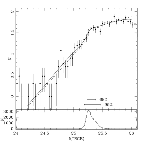
Figure 6: Similar to Fig. 3 but for NGC 4258

References

- (1) Aaronson, M., Bothun, G., Mould, J., Huchra, J., Schommer, R.A., Cornell, M.E., 1986, ApJ, 302, 536
- (2) Aguilar, L., Hut, P., & Ostriker, J.P., 1988, ApJ, 335, 720
- (3) Babu, G.J., & Feigelson, E.D., ed. 1996, Astrostatistics interdisciplinary statistics
- (4) Blecha, A., 1986, A&A, 154, 321
- (5) Comerón, F., Torra, J., Méndez, R.A., Gómez, A.E., 2001, A&A, 366, 796
- (6) Caputo, F., Marconi, M., Musella, I., 2002, ApJ, 566, 833
- (7) Carney, B.W., 1993, in The Globular cluster-Galaxy connection, eds. Smith, G.H., & Brodie J.P., ASP Conf. Ser., 234
- (8) Chiosi, C., Bertelli, G., & Bressan, A., 1992, ARA&A, 30, 235
- (9) Ciardullo, R., et al. , 2002, ApJ, 577, 31
- (10) Cioni, M.-R.L, van den Marel, R.P., Loup, C., & Habing, H.J., 2000, A&A, 359, 601
- (11) Da Costa, G.S., & Armandroff, T.E., 1990, AJ, 100, 162
- (12) Davidge, T.J., & Pritchet, C.J., 1990, AJ, 100, 102
- (13) Davidge, T.J., Le Fèvre, O., & Clark, C.C., 1991, ApJ, 370, 559
- (14) Dohm-Palmer, R.C., Helmi, A., Marrison, H., et al., 2001, ApJ, 555, L37
- (15) Dolphin, A.E., 2000, PASP, 112, 1397
- (16) Durrell, P.R., Harris, W.E., & Pritchet, C.J., 2004, AJ, 128, 260
- (17) Efron, B., & Tibshirani, R., 1986, Stat. Sci, 1, 54
- (18) Eggen, O., Lynden-Bell, D., & Sandage A., 1962, ApJ, 136, 748
- (19) Ferrarese, L., Mould, J.R., Kennicutt, R.C., Jr., et al., 2000, ApJS, 128, 431
- (20) Freedman W.L., et al. 2001, ApJ, 553, 47
- (21) Freeman, K.C., 1987, ARA&A, 25, 603
- (22) Freeman, K.C., & Bland-Hawthorn, J., 2002, ARA&A, 40, 487
- (23) Fruchter, A.S., & Hook, R.N., 2002, PASP, 114, 144
- (24) Greenhill, L.J., Jiang, D.R., Moran, J.M., Reid, M.J., Lo, K.Y., Claussen, M.J., 1995, ApJ, 440, 619
- (25) Gregg, M.D., Ferguson, H.C., Minniti, D., Tanvir, A., Catchpole, R., 2004, ApJ, 127, 1441
- (26) Grillmair, C.J., Freeman, K.C., Irwin, M., Quinn, P.J., 1995, AJ, 109, 2553
- (27) Groenewegen, M.A.T., Salaris, M., 2001, A&A., 366, 752
- (28) Heckman T.M., Armus L., & Miley G.K., 1990, ApJS, 74, 833
- (29) Herrnstein J.R., et al., 1999, Nature, 400, 539
- (30) Ho, L.C., Filippenko A.V., Sargent W.W, 1996, ApJ, 462, 183
- (31) Holtzman J.A. et al., 1995, PASP, 107, 1065
- (32) Ibata, R.A., Gilmore, G., & Irwin M.J., 1994, Nature, 370, 194
- (33) Ibata, R.A., Irwin M.J., Lewis, G., Ferguson, A.M.N., & Tanvir, N., 2001, Nature, 412, 49
- (34) Ivezic, Z., Goldston, J., Finlator, K., et al., 2000, ApJ, 120, 963
- (35) Karachentsev, I.D., & Drozdovsky, I.O., 1998, A&AS, 131, 1
- (36) Karachentsev, I.D., Sharina, M.E., Dolphin, A.E., et al., 2002, A&A, 385, 21
- (37) Knox, L., Christensen, N. & Skordis, C., 2001, ApJ, 563, L95
- (38) Krist, J., 2004, TinyTim manual, http://www.stsci.edu/software/tinytim/tinytim.pdf
- (39) Lee, M.G., Freedman, W.L., & Madore, B.F. 1993, ApJ, 417, 553
- (40) Lipari, S., Tsvetanov, Z., Macchetto, F., 1997, ApJS, 111, 369
- (41) Madore, B.F., & Freedman, W.L. 1995, AJ, 109, 1645
- (42) Marconi, A., Oliva, E., van der Werf, P.P., Maiolino, R., Schreier, E.J., Macchetto, F., Moorwood, A.F.M., 2000, A&A, 357, 24
- (43) Mendez, B., Davis, M., Moustakas, J., Newman, J., Madore, B.F., & Freedman W.L., 2002, ApJ, 124, 213
- (44) Miyoshi, M., Moran, J., Herrnstein, J., Greenhill, L., Nakai, N., Diamond, P., & Inoue, M., 1995, Nature, 373, 127
- (45) Maoz, E., 1995, ApJ, 455, 131
- (46) Maoz D., et al., 1999, Nature, 401, 351
- (47) Metropolis, N., Rosenbluth, A. W., Rosenbluth, M. N., Tellar, A. H., & Tellar, E., 1953, Journal of Chemical Physics, 21, 6.
- (48) Moorwood, A.F.M., et al. 1996, A&A, 308, L1
- (49) Morrison, H.L., 1993, AJ, 106, 578
- (50) Nelder, J. A. & Mead, R., 1965, Computer Journal, 7, 308
- (51) Newman J.A., et al., 2001, ApJ, 553, 562
- (52) Olling, R.P., 1996, AJ, 112, 481
- (53) Panagia, N., Gilmozzi, R., Macchetto, F., Adorf, H.-M., & Kirshner, R.P., 1991, ApJ, 380, L23
- (54) Perrett, K.M., Bridges, T.J., Hanes, D.A., et al., 2002, AJ, 123, 2490
- (55) Pietsch, W., Vogler, A., Klein, U., & Zinnecker, H., 2000, A&A, 360, 24
- (56) Press, W.H., Teukolsky, S.A., Vetterling, W.T. & Flannery, B.P., 1992, Numerical Recipes in C, Cambridge University Press, Cambridge.
- (57) Puche, A., & Carignan, C., 1988, AJ, 95, 1025
- (58) Radovich, M., Kahanpaa, J., Lemke, D., 2001, A&A, 377, 73
- (59) Renzin, A., 1992, in IAU Symp. 149, The Stellar Populations in Galaxies, Ed. B. Barbuy & A. Renzini (Dordrecht: Kluwer) 235
- (60) Rozanski R., & Rowan-Robinson, M., 1994, MNRAS, 271, 530
- (61) Sakai, S., Madore, B.F., & Freedman, W.L. 1996, ApJ, 461, 713
- (62) Sakai, S., Madore, B.F., Freedmen, W.L., Lauer, T.R., Ajhar, E.A., & Baum, W.A., 1997, ApJ, 478, 49
- (63) Sakai, S., Zaritsky, D., Kennicutt, R.C., Jr., 2000, AJ, 119, 1197
- (64) Salaris, M., & Cassisi, S., 1997, MNRAS, 289, 406
- (65) Salaris, M., & Girardi, L., 2005, MNRAS, 357, 669
- (66) Searle, L., & Zinn R., 1978, ApJ, 225, 357
- (67) Schlegel, D.J., Finkbeiner, D.P., & Davis, M., 1998, ApJ, 500, 525
- (68) Strickland, D.K., Heckman, T.M., Weaver, K.A., Hoopes, C.G., Dahlem, M., 2002, ApJ, 568, 689
- (69) Tikhonov, N.A., Galazutdinova, O.A., & Drozdovsky, I.O., 2005, A&A, 431, 127.
- (70) Tikhonov, N.A., & Galazutdinova, O.A., 2005, Astrofizica, in press, astro-ph/0503235.
- (71) Watson, W.D., & Wallin, B.K., 1994, ApJ, 437, L35
- (72) Verde, L., et al., 2003, ApJS, 148, 195.
- (73) Yanny, B., Newberg, H.J., Kent, S., et al., 2000, ApJ, 540, 825
- (74) Zoccali, M., & Piotto, G., 2000, A&A, 358, 943