The Discordance of Mass-Loss Estimates
for Galactic O-Type Stars

Abstract

We have determined accurate values of the product of the mass-loss rate and the ion fraction of P ⁴⁺, $\dot{M}q$(P ⁴⁺), for a sample of 40 Galactic O-type stars by fitting stellar-wind profiles to observations of the P v resonance doublet obtained with FUSE, ORFEUS/BEFS, and Copernicus. When P ⁴⁺ is the dominant ion in the wind (i.e., 0.5 $\lesssim$ $q$(P ⁴⁺) $\leq$ 1), $\dot{M}q$(P ⁴⁺) approximates the mass-loss rate to within a factor of $\lesssim$2. Theory predicts that P ⁴⁺ is the dominant ion in the winds of O7–O9.7 stars, though an empirical estimator suggests that the range from O4–O7 may be more appropriate. However, we find that the mass-loss rates obtained from P v wind profiles are systematically smaller than those obtained from fits to H$\alpha$ emission profiles or radio free-free emission by median factors of $\sim$130 (if P ⁴⁺ is dominant between O7 and O9.7) or $\sim$20 (if P ⁴⁺ is dominant between O4 and O7). These discordant measurements can be reconciled if the winds of O stars in the relevant temperature range are strongly clumped on small spatial scales. We use a simplified two-component model to investigate the volume filling factors of the denser regions. This clumping implies that mass-loss rates determined from “$\rho^{2}$” diagnostics have been systematically over-estimated by factors of 10 or more, at least for a subset of O stars. Reductions in the mass-loss rates of this size have important implications for the evolution of massive stars and quantitative estimates of the feedback that hot-star winds provide to their interstellar environments.

1 Introduction

The stellar winds from OB-type stars exert strong, dynamic influences on the evolution of massive stars and their interstellar environments. From the perspective of stellar evolution, continuous mass-loss via these outflows alters both the path of the star through the H-R diagram and the rate at which it is traversed. The continual shedding of the outer layers of the atmosphere also causes systematic changes in the chemical composition of the photosphere, particularly in the presence of strong, rotationally-induced mixing. Additionally, the injection of chemically enriched material, momentum, and energy from the winds of hot, massive stars into their surroundings is an integral part of the “stellar feedback” cycle, which mixes the local interstellar medium and ultimately drives the chemical evolution of a galaxy.

In view of their fundamental astrophysical importance, it is clear that the properties of these outflows must be well determined. Nowadays, it is understood that hot-star winds are driven by the transfer of momentum from the stellar radiation field through scattering in metallic resonance lines. However, ab initio models still require numerous assumptions in order to provide testable predictions of wind parameters. Consequently, empirical confirmation of the theory remains essential. For this purpose, the three most useful diagnostics of mass loss are, in order of increasing sensitivity: (a) free-free continuum emission at radio wavelengths; (b) H$\alpha$ line emission; and (c) ultraviolet (UV) resonance-line absorption. These diagnostics sample different parts of the wind, from the dense, near-star, rapidly accelerating region (H$\alpha$) to the very distant, rarefied, constant velocity regions (free-free radio emission) and essentially everywhere between (UV resonance lines). Their physical mechanisms have different dependencies on the local density (emission $\propto\rho^{2}$; absorption $\propto\rho$), while the measurable properties associated with each suffer different degrees of contamination from photospheric or other processes, and require different ancillary knowledge of, e.g., the excitation or ionization conditions in the wind, the velocity structure of the wind, or the distance to the star.

The need for additional information concerning the ionization structure of the wind has traditionally been a stumbling block for determinations of the mass-loss rates ($\dot{M}$) from the wind profiles of UV resonance lines. The problem arises because the strength of these profiles is determined by the radial optical depth of the wind, $\tau_{rad}\propto\dot{M}q_{i}A_{E}$, where $A_{E}$ and $q_{i}$ are the abundance of element $E$ and its ionization fraction for stage $i$. Thus, wind-profile modeling of a dominant ion ($q_{i}\sim 1$) of known abundance is required to estimate $\dot{M}$ directly. Unfortunately, the lines of dominant ions are usually saturated, particularly those for cosmically abundant elements (e.g., C, N, O) in winds that are sufficiently dense to provide reliable determinations of $\dot{M}$ from “density squared” [hereafter “$\rho^{2}$” and $\dot{M}$($\rho^{2}$)] diagnostics. As a result, only UV wind lines from trace ionization species with $q_{i}\lesssim 10^{-3}$ can typically be used to measure $\dot{M}q$ for massive winds, and values of $\dot{M}$ estimated from these measurements are compromised by the lack of a priori information needed to estimate $q_{i}$ accurately; see Lamers et al. (1999) for additional discussion of this problem. Thus, even though UV wind lines are the most sensitive indicators of $\dot{M}$ in early-type stars, empirical mass-loss rates have relied primarily on measurements $\dot{M}$($\rho^{2}$) from free-free radio emission [$\dot{M}$(radio)] and H$\alpha$ line emission [$\dot{M}$(H$\alpha$)]; see, e.g., Lamers & Leitherer (1993) or Puls et al. (1996).

Although mass-loss rates determined from radio measurements are usually regarded as the most reliable, comparatively few OB-type stars have been detected owing to the inherent weakness of free-free emission and its “$\rho^{2}$” dependence, which requires stars to be relatively nearby. In contrast, H$\alpha$ emission, which is also a “$\rho^{2}$” processes, can be easily observed in distant objects. However, because its strength depends on the details of the wind–photosphere interface, it is more difficult to model, although the current consensus is that mass-loss rates determined from H$\alpha$ are quite accurate (Puls et al., 1996).

Access to the far-ultraviolet region of the spectrum provided by the Far Ultraviolet Spectroscopic Explorer (FUSE) affords a renewed opportunity to examine the use of resonance-line diagnostics for the determination of $\dot{M}$, and to perform consistency checks on measurements of $\dot{M}$($\rho^{2}$). For this purpose, the P v $\lambda\lambda$1118, 1128 doublet plays a pivotal role, primarily because P ⁴⁺ is expected to be the dominant ion the winds of some O stars. This expectation is based on naive energetic considerations, morphological trends observed in the spectra of O stars, and detailed modeling. From a diagnostic perspective, an equally important attribute of P ⁴⁺ is that, despite its high ionic abundance, the P v $\lambda\lambda$1118, 1128 doublet is rarely saturated because the cosmic abundance of P is so small. On the other hand, this also means that the wind contribution to the doublet is only measurable in stars with massive winds. Finally, in contrast to C, N, and O, P is not produced by H-burning; consequently its atmospheric abundance does not change substantially over a stellar lifetime or as a function of the vigor of rotational mixing. Thus, star-to-star changes in its abundance should not contribute to the cosmic scatter in $\dot{M}$ determinations.

These properties make the P v resonance doublet a powerful mass-loss diagnostic for a range of O-star temperature classes, though we expect the detection of wind profiles in the P v resonance doublet to be biased toward stars with more massive winds. If we simply assume that $q$(P ⁴⁺) approaches unity in stellar winds somewhere in the O star range, then values of $\dot{M}q$(P ⁴⁺) should agree with both $\dot{M}$(radio) and $\dot{M}$(H$\alpha$) for at least some O stars. If concordance between these individually reliable mass-loss indicators is not found, then their different formation mechanisms will help to constrain the reasons for the discrepancy. Massa et al. (2005) reported on a preliminary comparison between these different measures of $\dot{M}$, and the current paper expands and refines that work.

In the present study, we have measured $\dot{M}q({\rm P}^{4+})$ for a sample of 40 well-studied Galactic O-type stars that have reliable radio or H$\alpha$ mass-loss measurements available from the literature. This sample is described in §2. New FUSE observations and wind-profile analysis of all P v resonance doublets are described in §3.1 and 4.3, respectively. The values of $\dot{M}q$ derived for P ⁴⁺ are compared with the values of $\dot{M}$($\rho^{2}$) in §5, and large discrepancies are found. Possible reasons for this discordance are discussed in §6, before the main conclusions from this study are summarized in §7.

2 The Sample

Table The Discordance of Mass-Loss Estimates for Galactic O-Type Stars lists the sample of Galactic O-type stars used in this investigation. The sample is defined by the availability of (a) reliably determined values of the fundamental stellar parameters; (b) reliable determinations of $\dot{M}$ from thermal radio emission or H$\alpha$ emission profiles; and (c) far-UV spectra that include the P v resonance lines. For practical purposes, the first two criteria limit the selection of objects to those that have been well-studied over the past decade by the methods of “quantitative spectroscopy.” These objects serve as a fundamental data set, and are the cornerstone for the calibration of the Wind-Momentum-Luminosity relation for Galactic O stars (Puls et al., 1996; Repolust et al., 2004). The sample spans all subclasses of O-type spectra, but is biased toward higher luminosity classes. The luminosity bias occurs because both “$\rho^{2}$” diagnostics and the P v wind features are preferentially detected in the densest outflows, which are associated with more luminous objects.

2.1 Stellar Parameters

As described in §4.3, determinations of $\dot{M}q$(P ⁴⁺) from the P v resonance lines requires knowledge of the stellar radius, $R_{\star}$; the projected rotational velocity, $v\sin i$, which determines the width of the photospheric lines; and the terminal velocity of the stellar wind, ${v}_{\infty}$. These parameters and their origin are indicated in Table The Discordance of Mass-Loss Estimates for Galactic O-Type Stars, along with the spectral type and the adopted values of $T_{\rm eff}$.

To minimize possible systematic biases in the derived stellar parameters, the sample is subdivided into “primary” (28 objects) and “secondary” (12 objects) subsets according to how the parameters were determined. Most of the determinations for the primary data set come from the work of Repolust et al. (2004), which provides the largest sample of homogeneously determined stellar parameters currently available for Galactic O stars. These are derived from fits made with the unified (i.e., photosphere $+$ wind), non-LTE, line-blanketed model atmosphere program FASTWIND (Puls et al., 2005). The primary sample also contains objects analyzed by Markova et al. (2004) with a more simplified approach, which relies in part on calibrations of fundamental parameters derived from the work of Repolust et al. (2004). Thus, the values of the derived stellar parameters for the primary sample are internally consistent and incorporate recent revisions to the temperature scale associated with O-type stars (Martins et al., 2002; Crowther et al., 2002; Bianchi & Garcia, 2002; Herrero et al., 2002; Martins et al., 2005).

Since similar fits with unified model atmospheres are not yet available for stars in the secondary sample, the values of $T_{\rm eff}$ and $R/R_{\sun}$ listed for them in Table The Discordance of Mass-Loss Estimates for Galactic O-Type Stars are based on the revised spectral-type calibrations presented by Martins et al. (2005). The parameters given for the “observational scale” (i.e., Tables 4–6 of Martins et al., 2005) were used to minimize possible systematic differences with the primary sample. Values for luminosity class II were estimated by linear interpolation between luminosity classes I and III; and the parameters associated with O9.5 supergiants were adopted for the three O9.7 supergiants in the secondary sample. Of course, it would be very useful to determine the stellar parameters of all the stars listed in Table The Discordance of Mass-Loss Estimates for Galactic O-Type Stars through rigorously uniform analysis.

Table The Discordance of Mass-Loss Estimates for Galactic O-Type Stars also notes which objects in the sample are known or suspected binary stars, as designated in the Galactic O-Star Catalog (Maíz-Apellániz et al., 2004).

3 Far-Ultraviolet Spectra

The far-UV spectra used to measure the P v wind profiles of the targets in the sample were acquired by several observatories. These are indicated in Table 2, along with other salient details concerning the observations. Most of the spectra were obtained with FUSE, either as part of our Guest Investigator program E082, which was dedicated to measurements of P v, or as a by-product of programs devoted to other topics. The processing of these data is described in §3.1.

Owing to count-rate limits associated with the FUSE detectors, bright objects are difficult or impossible to observe. Consequently, FUSE cannot observe nearby, unreddened O stars. This is unfortunate, since these are generally the objects that have received the most attention from ground-based observers and for which radio mass-loss rates are available. For these bright stars, we have used archival far-UV spectra that were obtained by Copernicus or the Berkeley Extreme and Far-UV Spectrometer (BEFS). These spectra were retrieved from the Multi-Mission Archive at the Space Telescope Science Institute (MAST). The data sets for these instruments are indicated in Table 2, and were used without further manipulation.

3.1 FUSE Observations and Reduction

The FUSE observatory consists of four aligned, prime-focus telescopes and Rowland-circle spectrographs that feed two photon-counting detectors (Moos et al., 2000; Sahnow et al., 2000). These four channels provide redundant coverage of the range between $\sim 905-1187$ Å. As indicated in Table 2, most objects were observed through the large 30″$\times$ 30″(LWRS) aperture. The lone exception is HD 188209, which was observed through the narrow 1.25″$\times$ 20″(HIRS) aperture as part of a test of observing techniques for bright objects.

The FUSE spectra were uniformly extracted and calibrated with CalFUSE version 2.4.2. Subsequent processing used the shifts determined by cross-correlating the positions of sharp interstellar features to align the spectra extracted from individual exposures; resampled the spectra onto a uniform wavelength grid with steps of 0.1 Å; and normalized the profiles to the local stellar continuum. Since normalization of LiF1B spectra acquired through the LWRS aperture is complicated by an optical artifact known as “the worm” (Sahnow, 2002), we used the redundant and cleaner coverage of the P v doublet provided by LiF2A spectra whenever possible.

4 Mass-Loss Determinations

Determinations of the mass-loss rates for O stars traditionally assume that the wind is a spherically symmetric, steady, homogeneous, and monotonically expanding outflow. All the measurements discussed in this section depend on these underlying assumptions of this “standard wind model.”

4.1 H$\alpha$ Measurements

Most of the stars in the sample have $\dot{M}$(H$\alpha$) measurements. The bulk of these were obtained from comparisons with FASTWIND calculations of the entire optical spectrum by Repolust et al. (2004), which were also used to derive other fundamental stellar parameters. Since these computations help to define the revised temperature scale, the values of $\dot{M}$(H$\alpha$) are completely consistent with it.

An important subset of objects have $\dot{M}$(H$\alpha$) determined from fits to only the H$\alpha$ line profile by Markova et al. (2004). They used the quick but accurate method developed by Puls et al. (1996). These measurements rely in part on calibrations of stellar parameters as a function of spectral type that were based on the complete modeling of Repolust et al. (2004). Markova et al. (2004) show that their results are internally consistent with the values derived from the more complete analysis.

Less reliable estimates of $\dot{M}$(H$\alpha$) were used for four stars in the secondary sample: HD 45160, HD 46223, HD 164794, and HD 188001. For these stars, $\dot{M}$ was determined by Puls et al. (1996, their Table 11) from a re-analysis of the equivalent width measurements compiled by Lamers & Leitherer (1993). These values are not of comparable quality to the other determinations used here, since they (a) rely on equivalent widths rather than fits to the entire line profile; (b) are in some cases obtained from measurements of photographic plates, which are inherently less precise than the CCD data used by Repolust et al. (2004) and Markova et al. (2004); and (c) were interpreted on the basis of a temperature scale that is systematically hotter than the one used for the bulk of the stars analyzed here. Since three of these targets (HD 46150, HD 46223, HD 164794) only have upper limits for $\dot{M}q$(P ⁴⁺), the greater uncertainty inherent in their values of $\dot{M}$(H$\alpha$) does not affect the comparison significantly. The fourth star, HD 188001, is the only program star in this group with detections of both $\dot{M}$(H$\alpha$) and $\dot{M}q$(P ⁴⁺). Although the $T_{\rm eff}$ of this star has been adjusted in Table The Discordance of Mass-Loss Estimates for Galactic O-Type Stars, its value of $\dot{M}$(H$\alpha$) has not been rescaled.

4.2 Measurements of Radio Free-Free Emission

Mass-loss rates determined from radio free-free emission are available for 40% of the stars in the sample. Most of these have been taken from the compilation of Lamers & Leitherer (1993), who provide a thorough discussion of this technique. These results are supplemented by the more recent detections of HD 14947 and HD 190429A by Scuderi et al. (1998). Following the procedure adopted by Lamers & Leitherer (1993), the uncertainties quoted by Scuderi et al. (1998) have been increased by $\pm$0.10 dex to account approximately for uncertainties in the distance to the objects.

However, all these determinations pre-date the revisions to the effective temperature scale for O stars. At first sight, $\dot{M}$(radio) seems immune from these changes, since $T_{\rm eff}$ enters the expression for $\dot{M}$ explicitly only very weakly as a logarithmic contribution to the Gaunt factor; see, e.g., equation (5) of Lamers & Leitherer (1993). In fact, the resultant changes in $M_{V}$ and stellar luminosity generally result in different estimates for the distance, $d$, to the various stars; see, e.g., Martins et al. (2005). Since $\dot{M}$(radio) $\propto d^{1.5}$, a systematic difference results between $\dot{M}$(H$\alpha$) (which, except for HD 188001, are on the cooler temperature scale) and $\dot{M}$(radio).

To account for this dependence, we have systematically adjusted the values of $\dot{M}$(radio). For stars in the primary sample, we used the value of $M_{V}$ quoted by Repolust et al. (2004) and Markova et al. (2004), together with photometry from the Galactic O-Star Catalog (Maíz-Apellániz et al., 2004), to estimate the distance modulus via the standard formula

$$DM=V-M_{V}-3.1\,E(B-V)$$ (1)

This leads to a revised estimate of the distance, $d_{new}$, and a correction factor for the published value of $\dot{M}$(radio) of $f_{corr}=(d_{new}/d_{old})^{1.5}$, where $d_{old}$ was listed by Lamers & Leitherer (1993) or Scuderi et al. (1998). The same approach was followed for stars in the secondary sample, though in this case internally consistent values of $M_{V}$ were adopted from the spectral-type calibration of Martins et al. (2005). Table The Discordance of Mass-Loss Estimates for Galactic O-Type Stars lists the correction factors that were applied to make the measurements of $\dot{M}$(radio) consistent with the measurements of $\dot{M}$(H$\alpha$).

4.3 P v Wind-Profile Fitting

The strength of the absorption trough of a P Cygni wind profile at any normalized velocity $w=v/v_{\infty}$ (where ${v}_{\infty}$ is the terminal velocity of the wind) depends on the radial optical depth of material along the line-of-sight at that velocity, $\tau_{rad}(w)$, which is directly related to the column density.

For the P v resonance lines (whose basic properties are listed in Table The Discordance of Mass-Loss Estimates for Galactic O-Type Stars), $\tau_{rad}(w)$ for each program star was determined by using the “Sobolev with Exact Integration” (SEI; Lamers et al., 1987) wind-profile fitting technique with the modifications described by Massa et al. (2003). These modifications permit the relationship between optical depth and position in the absorption trough to be an arbitrary function, and also allow approximately for the effects of interstellar absorption, whenever required. The analysis proceeded in three steps.

First, the parameters of the velocity law were defined. The velocity law, $w(x)$, was parameterized in terms of the usual $\beta$-law by

$$w(x)=w_{0}+(1-1/x)^{\beta}~{}~{}$$ (2)

where $w=v/v_{\infty}$ is the normalized velocity; $x=r/R_{\star}$ is the radial distance in units of the stellar radius; and where the radial gradient is controlled by the parameter $\beta$, which is typically $\sim$1. The adopted values of ${v}_{\infty}$ are listed in Table The Discordance of Mass-Loss Estimates for Galactic O-Type Stars. These were determined from the shape of strongly saturated P Cygni profiles, typically the C iv $\lambda\lambda$1548, 1550 doublet, and included an estimate of any additional velocity dispersion (often referred to as “turbulence”) in the wind, which is usually required to reproduce the slope of the blue edge of the absorption trough. We found that adopting a value of 0.05 ${v}_{\infty}$ for this additional velocity dispersion was sufficient to model the P v profiles. Similarly, we adopted $\beta=1$ for all initial fits to the P v doublet, and altered it by modest amounts only if significantly better fits resulted. The final values of $\beta$ are listed in Table The Discordance of Mass-Loss Estimates for Galactic O-Type Stars.

Second, the P v doublet in each spectrum was fitted with the adopted velocity law by adjusting the optical depth in the radial direction, $\tau_{rad}(w)$, in $\sim$20 velocity bins distributed through the absorption trough. As explained in detail by Massa et al. (2003), determining the optical depth in absorption in a given bin also determines the contribution to blue- and red-shifted emission, so that a satisfactory fit to the entire profile is constructed by stepping through the absorption trough from its blue edge to line center. Underlying photospheric profiles were approximated by Gaussians, but since their influence is confined to low velocities (within $\pm$$v\sin i$; see Table The Discordance of Mass-Loss Estimates for Galactic O-Type Stars for the adopted values), their inclusion has little effect on the determination of $\tau_{rad}(w)$ for $w\gtrsim 0.2$, except in cases where the wind profile is extremely weak. A bigger problem is the blend of P v $\lambda$1128 with a strong, excited transition of Si iv in the spectra of later O-type stars. In these cases, greater weight was given to the P v $\lambda$1118 profile. Figures 1 and 2 illustrate the quality of the fits for a selection of targets.

Third, these determinations of $\tau_{\rm rad}(w)$ were used to compute $\dot{M}q({\rm P}^{4+};w)$ for each star from the relation:

$$\dot{M}q({\rm P}^{4+};w)=\left(\frac{m_{e}c}{\pi e^{2}}\right)\frac{4\pi\mu m_{H}}{f_{ij}\lambda_{0}A_{P}}R_{\star}v_{\infty}^{2}x^{2}w\frac{dw}{dx}\tau_{rad}(w)$$ (3)

where $f_{ij}$ is the oscillator strength of the appropriate component of the P v resonance line; $A_{P}$ is the abundance of P relative to hydrogen by number (Table The Discordance of Mass-Loss Estimates for Galactic O-Type Stars); $\mu$ is the mean molecular weight of the plasma; and all other symbols have their usual meaning. In equation (3), we adopted $\mu=1.34$ (appropriate for a completely ionized plasma of solar abundance), together with the values of $R_{\star}$ and ${v}_{\infty}$ listed in Table The Discordance of Mass-Loss Estimates for Galactic O-Type Stars. The measurements of $\dot{M}q_{i}(w)$ were averaged over normalized velocities between 0.2 and 0.8 to obtain the values of $\dot{M}q$(P ⁴⁺) listed in Table The Discordance of Mass-Loss Estimates for Galactic O-Type Stars.

The errors associated with the derived $\tau_{rad}(w)$ depend on its magnitude. For $\tau_{rad}(w)\lesssim 0.05$, the error can be as large as a factor of two. Similarly, for $\tau_{rad}(w)\gtrsim 2.0$ the error can also be large, while for $\tau_{rad}(w)\sim 1.0$, it is on the order of 10%. Consequently, we provide only upper limits for lines whose blue (stronger) component has an optical depth less than 0.05. None of the program stars has an optical depth in the red (weaker) component of the P v doublet greater than 2.0, so there is no need to define lower limits on $\tau_{rad}(w)$. Typical errors in parameters derived from the integrated optical depths, such as $\dot{M}q$(P ⁴⁺), are $\lesssim 25$%, and only quantities derived from the weakest lines have significantly larger errors. The value of $\beta$ can also affect $\tau_{rad}(w)$. However, $\beta$ is typically determined to within $\pm 0.2$, and uncertainties of this amount have very little effect on $\tau_{rad}(w)$ over the range $0.2\leq w\leq 0.8$.

5 Results

5.1 Comparison of $\dot{M}$($\rho^{2}$) with $\dot{M}q$(P ⁴⁺)

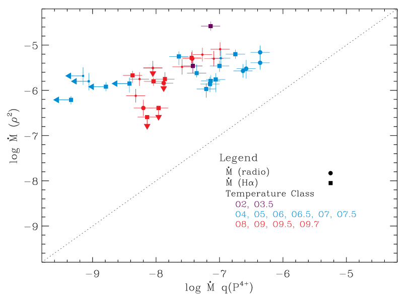
Figure 3: Comparison of $\dot{M}$ with $\dot{M}q$(P ⁴⁺). The shapes of symbols distinguish radio (circles) and H$\alpha$ measurements, while symbol size separates the primary (large) and secondary (small) samples. Upper limits on non-detections are indicated by arrows. Color coding divides the entire sample into early- (O2, O3, O3.5), mid- (O4–O7.5), and late-O types (O8–O9.7). The dotted line denotes a 1–1 correlation between the two measurements.

The published values of $\dot{M}$(radio) [modified as described in §4.2] and $\dot{M}$(H$\alpha$) are listed in Table The Discordance of Mass-Loss Estimates for Galactic O-Type Stars. They are compared with the average values of $\dot{M}q$(P ⁴⁺) in Figure 3 as a function of spectral type, measurement technique, and status as members of the primary or secondary sample. When more than one $\dot{M}$($\rho^{2}$) measurement was available, $\dot{M}$(radio) was preferred, except in cases where the uncertainties associated the $\dot{M}$(H$\alpha$) measurement were substantially smaller. Since only upper limits on both $\dot{M}$($\rho^{2}$) and $\dot{M}q$(P ⁴⁺) are available for HD 46150 and HD 217086, the values for these stars are not plotted in Fig. 3. The position of HD 149757 is not indicated either, since its very small value of $\dot{M}q$(P ⁴⁺) lies beyond the limits of the plot.

Several things are apparent from Figure 3. First, $\dot{M}q$(P ⁴⁺) is systematically smaller than $\dot{M}$($\rho^{2}$) by substantial amounts. Second, the size of the deviation does not depend on whether the fiducial $\dot{M}$($\rho^{2}$) was $\dot{M}$(radio) or $\dot{M}$(H$\alpha$). Third, any biases in the determinations of $\dot{M}$ for stars in the secondary sample are much smaller than the systematic deviations from the line indicating a 1–1 correlation. Finally, a strong dependence on binarity is not evident.

However, systematic trends in the distribution of deviations with spectral class are apparent. The sample can be divided into three parts:

1. The mid O-type stars (O4 – O7.5) with strong wind features (i.e., those with $\log$ $\dot{M}q$(P ⁴⁺) $\geq-8$) exhibit the smallest deviations from the values of $\dot{M}$(H$\alpha$) or $\dot{M}$(radio).

2. The earliest (O2–O3.5) and latest (O8–O9.7) O stars exhibit systematically larger deviations from the 1–1 correlation line.

3. The largest deviations belong to a group of five mid-O dwarfs and giants that have $\dot{M}$(H$\alpha$) measurements, and only upper limits for $\dot{M}q$(P ⁴⁺). These stars are (from left to right in Fig. 3: HD 42088 (O6.5 V), HD 46223 [O4 V((f+))], HD 47839 [O7 V((f))] HD 217086 (O7 Vn), and HD 203064 [O7.5 III:n((f))].

Figure 4 presents an alternate representation of this discrepancy in terms of an empirical estimate of the mean value of $q$(P ⁴⁺),

$$q_{\rm est}\equiv\dot{M}\,q({\rm P^{4+}})/\dot{M}(\rho^{2})~{}.$$ (4)

In Fig. 4, $q_{\rm est}$ is plotted as a function of $T_{\rm eff}$ for different luminosity classes. Although expected to be near unity over some range of $T_{\rm eff}$, it is never more than $\sim$0.11 for supergiants, and becomes progressively smaller for less luminous stars (0.06 for giants; 0.04 for dwarfs). Thus, $\dot{M}$($\rho^{2}$) is systematically larger than $\dot{M}q$(P ⁴⁺), as also indicated in Fig. 3. Since the initial expectation was that $\dot{M}q$(P ⁴⁺) should be nearly equal to $\dot{M}$($\rho^{2}$) for at least some O-type stars, the size and systematic nature of the deviations requires explanation.

5.2 For Which Stars is P ⁴⁺ Dominant?

A crucial assumption implicit in our emphasis on P v is that $q$(P ⁴⁺) $\approx$ 1 for O stars spanning some range of $T_{\rm eff}$. Apart from naive energetic considerations, this assumption is supported by detailed model atmosphere calculations. In particular, smooth-wind models computed with FASTWIND indicate that this temperature range is $\sim$31 – 34 kK, which corresponds to spectral types between O9.7 – O7.5 for supergiants and O9.5 – O8.5 for dwarfs.

However, the distribution of the empirical estimates of $q$(P ⁴⁺) in Fig. 4 suggests that the appropriate range of $T_{\rm eff}$ might be shifted to hotter temperatures. For more luminous objects, $q_{\rm est}$ exhibits a broad maximum between $T_{\rm eff}$ $\sim$34 – 40 kK (i.e., O7.5 – O4; mid-range O stars). A peak near $\sim$41 kK may also be indicated for dwarfs, though the behavior of $q_{\rm est}$ is not very clear for these objects.

A simple interpretation of the distribution of $q_{\rm est}$ with $T_{\rm eff}$ is that it traces the rise and fall of P ⁴⁺ as the dominant ion in the wind. In this case, P ³⁺ would be the dominant ion for $T_{\rm eff}$$\lesssim$ 34 kK, while the balance shifts in favor of P ⁵⁺ for $T_{\rm eff}$$\gtrsim$ 40 kK. For both extremes, $q$(P ⁴⁺) $\ll$ 1, as implied by Fig. 4. However, this straightforward interpretation is complicated by the reliance of $q_{\rm est}$ on $\dot{M}$($\rho^{2}$). For example, biases in the determination of $\dot{M}$($\rho^{2}$) will also bias $q_{\rm est}$. Evidently a more systematic modeling effort will be required to determine the temperature range for which P ⁴⁺ is the dominant ion.

Irrespective of this uncertainty in the appropriate range of $T_{\rm eff}$, we conclude that there is a large, systematic discrepancy between $\dot{M}q$(P ⁴⁺) and the “$\rho^{2}$” determinations, $\dot{M}$(H$\alpha$) and $\dot{M}$(radio), for some O stars.

1. If, as predicted by standard FASTWIND models, P ⁴⁺ is dominant in the winds of O7.5 – O9.7 stars, then Table The Discordance of Mass-Loss Estimates for Galactic O-Type Stars indicates that the median discrepancy for the subset of 15 luminous (i.e., non-dwarf) stars with solid detections corresponds to $\dot{M}$($\rho^{2}$)/$\dot{M}q$(P ⁴⁺) = 129, with minimum and maximum values of 17 and 501 for HD 24912 and HD 209975, respectively.

2. If, as suggested by a straightforward interpretation of the behavior of $q_{\rm est}$ in Fig. 4, P ⁴⁺ is dominant for stars with spectral classes between O4–O7.5, the median discrepancy for the subset of 13 luminous stars with solid detections corresponds to $\dot{M}$($\rho^{2}$)/$\dot{M}q$(P ⁴⁺) = 20, with minimum and maximum values of 9 and 245 for HD 66811 and HD 15558, respectively.

5.3 Stars with weak winds

The extremely large discrepancies for the mid O-type stars with weak winds (i.e., the class III – V stars) are an interesting special case, which might result from systematic measurement errors in $\dot{M}$(H$\alpha$). None of these targets have obvious wind profiles in P v, so only upper limits for $\dot{M}q$(P ⁴⁺) can be estimated. Similarly, none of these stars are detected in the radio, and none exhibit bona fide H$\alpha$ emission profiles. As a result, these determinations of $\dot{M}$(H$\alpha$) depend sensitively on estimates of the degree to which the underlying photospheric profiles are partially filled by wind emission, which in turn relies critically on the accuracy of the photospheric models. Such wind contamination is clearly evident in the H$\alpha$ profiles of HD 203064 (Repolust et al., 2004), though emission from a circumstellar disk is not precluded for this rapid rotator. HD 217086 is also a rapid rotator, though in this case partial filling by emission is not evident, and only an upper limit on $\dot{M}$ was determined (Repolust et al., 2004). Emission is less evident in the H$\alpha$ profiles of HD 47839, which might instead be weakly contaminated by the spectrum of its late-O companion (Gies et al., 1993).

In any case, if the determinations of $\dot{M}$(H$\alpha$) for the less-luminous, mid O-type stars are taken at face value, they yield values that are inconsistent with the non-detection of wind profiles in the resonance lines of P v, at least for the assumed solar abundance of P. Although the magnitude of the discrepancy is indeterminate for these objects, the sense is the same as for the rest of the mid-O stars. The largest value of $\dot{M}q$(P ⁴⁺) for any main sequence O star in our sample is $7.2\times 10^{-8}$ ${\rm M}_{\sun}/{\rm yr}$, and most are less than this by an order of magnitude or more. Thus, if $q$(P ⁴⁺) ever approaches unity for main sequence O stars, then their mass-loss rates are much smaller than theoretical expectations, which are $\gtrsim 10^{-7}$ ${\rm M}_{\sun}/{\rm yr}$ for these stars (Vink et al., 2000).

5.4 Comparison of $\dot{M}$(radio) with $\dot{M}$(H$\alpha$)

Although not a primary motivation of the present study, the compilation of measurements of $\dot{M}$ data in Table The Discordance of Mass-Loss Estimates for Galactic O-Type Stars provides an opportunity to re-examine the agreement between measurements of $\dot{M}$(radio) and $\dot{M}$(H$\alpha$). Detections are available for both diagnostics for a subset of 8 objects. A comparison of the two measurements for these stars indicates a systematic difference between them, with the mean value of $\dot{M}$(H$\alpha$) / $\dot{M}$(radio) $\approx 2.4\pm 0.7$. This is contrary to previous studies (e.g., Lamers & Leitherer, 1993; Puls et al., 1996), which found agreement between the two measures. Blomme et al. (2003) noted a similar – though smaller – discrepancy between $\dot{M}$(radio) and $\dot{M}$(H$\alpha$) determinations for HD 66811 [O4 I(n)f].

6 Discussion

It has been known for some time (see, e.g., Hamann, 1980) that self-consistent wind models produce too much absorption in the P v resonance lines of individual O-types stars. Although the precise range of spectral types where $q$(P ⁴⁺) is dominant is poorly defined at present, the large sample considered here indicates that there is a significant, systematic discrepancy between mass-loss determinations for all objects with spectral types in either of the two possible ranges discussed in §5.2. Thus, the “P v problem” is not limited to a few, possibly peculiar objects. Instead, the discordance between $\dot{M}$ diagnostics indicates that one or more biases must be influencing the analyses in such a way that either $\dot{M}q$(P ⁴⁺) is systematically under-estimated, or that $\dot{M}$(radio) and $\dot{M}$(H$\alpha$) are systematically over-estimated. A combination of biases might also be affecting these diagnostics by different amounts. In the following sections, we examine the biases that might affect mass-loss rates determined by different methods within the context of the standard wind model (i.e., a smooth, steady, and spherically symmetric wind).

6.1 Biases in Measurements of $\dot{M}$(H$\alpha$)

A measurement of $\dot{M}$(H$\alpha$) is complicated, because it requires (a) accurate knowledge of the distribution of wind density in the near-star environment; (b) non-LTE calculations to determine the excitation equilibrium of H; and (c) an accurate model for the underlying photospheric feature, which must also incorporate the blend with He ii $\lambda$6560. The latter two requirements are both sensitive to temperature, with hotter temperatures usually leading to larger values of $\dot{M}$ (Puls et al., 1996). Consequently, values of $\dot{M}$(H$\alpha$) may be systematically over-estimated with old, hotter temperature scale. However, since only one of the older $\dot{M}$(H$\alpha$) measurements was used in Figs. 3 and 4 (see §4.1), this is unlikely to be an important bias. If anything, the reduction in the temperature scale should move values of $\dot{M}$(H$\alpha$) closer to $\dot{M}q$(P ⁴⁺).

A more subtle problem occurs for stars of luminosity class V–III, which typically exhibit a partially filled absorption profile rather than emission above the local continuum. For these stars, estimates of $\dot{M}$(H$\alpha$) depend very sensitively on how well the underlying photospheric profile is reproduced by the adopted model atmosphere. It is possible that small, systematic uncertainties in the strength of the photospheric H$\alpha$ profiles contribute to the large discrepancy between $\dot{M}q$(P ⁴⁺) and $\dot{M}$(H$\alpha$) exhibited by the group of 5 mid-range O dwarfs and giants seen in Fig. 3.

Another potential source of bias in determinations of $\dot{M}$(H$\alpha$) is the high frequency of variability (Ebbets, 1982; Kaper et al., 1998; Markova et al., 2005). Many of these variations are characterized by changes in the equivalent width of the emission, which implies that either the amount of material or its density distribution changes. Consequently, it is difficult to evaluate the extent to which a measurement based on a single profile at a snapshot in time represents the global, time-averaged mass flux. Wind-wind interactions in short-period binary systems also produce complicated variations in H$\alpha$; see, e.g., the series of papers bounded by Gies & Wiggs (1991) and Thaller et al. (2001). Although the effects of colliding winds are not included in the analyses used to compile Table The Discordance of Mass-Loss Estimates for Galactic O-Type Stars, there is no particular evidence that that binaries depart from the general trends evident in Fig. 3.

6.2 Biases in Measurements of $\dot{M}$(radio)

The $\dot{M}$(radio) are usually assumed to be the most reliable, since the physical mechanism responsible for the radio emission (free-free emission) is well understood; ionization corrections are generally insignificant (Lamers & Leitherer, 1993); and contamination from the stellar photosphere is completely negligible. Furthermore, the radio photosphere is typically sufficiently far from the star that the details of the velocity law are not important: only ${v}_{\infty}$ is required, which can be determined accurately from UV resonance lines. In the context of the standard wind model, the only other input to $\dot{M}$(radio) is the distance. Although imperfect knowledge of the distances to Galactic O stars introduces scatter into the derived $\dot{M}$(radio), the uncertainties should be random and are unlikely to result in a systematic bias.

However, it has been recognized for many years that the $\dot{M}$(radio) can be systematically over-estimated if a fraction of the observed radio flux is due to nonthermal emission. Approximately 25% of O-type stars exhibit nonthermal radio emission, which can be recognized either through dramatic variability between epochs or from the frequency dependence of their radio spectra (Bieging et al., 1989). Binarity may play a role in generating nonthermal electrons through wind-wind interactions; see, e.g., the recent discussion of radio observations of HD 93129A by Benaglia & Koribalski (2004). However, other mechanisms may contribute to the nonthermal radio emission from the winds of single stars; see, e.g., Van Loo et al. (2004). Of the 16 stars in our sample with $\dot{M}$(radio) measurements, only 3 are considered “definite” thermal emitters (HD 66811, HD 37742, and HD 152408) by Lamers & Leitherer (1993), and 2 more are considered “probable” thermal emitters (HD 30614 and HD 151804). The remaining 11 stars have measurements at a single frequency, which is insufficient to establish that the emission is thermal. Five of these objects are known or suspected binaries, although these stars do not appear to have systematically larger $\dot{M}$(radio) values compared to similar, single stars. Most of the stars with $\dot{M}$(radio) measurements also have $\dot{M}$(H$\alpha$) measurements that are larger still; see §5.4. Thus, it seems that any biases common to “$\rho^{2}$” diagnostics affect $\dot{M}$(H$\alpha$) more than $\dot{M}$(radio).

6.3 Biases in Measurements of $\dot{M}q$(P ⁴⁺)

Equation (3) shows that $\dot{M}q$(P ⁴⁺) will be systematically under-estimated if either the oscillator strength, $f_{ij}$, or the P abundance, $A_{P}$, is over-estimated. Although random errors in the other parameters required to evaluate equation (3) will introduce uncertainties, the resulting effects are unlikely to be systematic.

Since P ⁴⁺ is a lithium-like ion, it is quite unlikely that its oscillator strength is uncertain by a substantial amount. Morton (2003) does not indicate that there is any controversy related to the value of $f_{ij}$. Consequently, there is no reason to suspect that the oscillator strength biases measurements of $\dot{M}q$(P ⁴⁺).

The Galactic P abundance is more problematic. Some authors (e.g., Pauldrach et al., 1994, 2001) have adopted subsolar values (e.g., P/P_☉ of 0.50–0.67 and 0.05 for HD 66811 and HD 30614, respectively) in order to achieve good fits for wind profiles in the P v resonance doublet. However, there is little evidence to support a systematically reduced abundance of P for Galactic O-type stars. The solar P abundance by number relative to H is $A_{P}=12.00+\log(N_{P}/N_{H})=5.45\pm 0.06$ (Biemont et al., 1994)), which is $\sim$30% smaller than the meteoric abundance ($A_{P}=5.56$;  Anders & Grevesse, 1989). Dufton et al. (1986) measured $A_{P}=5.59$ in the Galactic interstellar medium from a survey of the P ii $\lambda\lambda$1153, 1302 resonance doublet along 51 sight lines and found that it was only modestly depleted (factors of 3 or less) in cold clouds. More recently, Lebouteiller et al. (2005) have also confirmed that the interstellar abundance of P is solar. Similarly, analysis of a FUSE spectrum of HD 207538 (B0 V, though a candidate for a chemically peculiar star) by Catanzaro et al. (2003) shows that the photospheric lines of P iv are well reproduced with solar abundances. Thus, there is no particular evidence that the abundance of P is systematically subsolar in the material from which O stars form, or in their cooler, B-type relatives. It is in principle possible to search for anomalous P abundances more explicitly by determining the photospheric abundance of P v from O-type stars with weak winds (e.g., HD 47839; see Fig. 2).

A more speculative explanation for the systematically small values of $\dot{M}q$(P ⁴⁺) is that $q$(P ⁴⁺) peaks for O stars at a value that is substantially less than 1. Of course, this behavior is not predicted by standard wind models, and would require that some unusual circumstances dominate the ionization balance of P. A candidate mechanism noted by Pauldrach et al. (1994) is the approximate coincidence of the ground-state ionization threshold of P v (65.023 eV; 191 Å) with that of He ii (54.416 eV; 228 Å). As a result, Pauldrach et al. (1994) speculated that $q$(P ⁴⁺) is driven by the behavior of He ⁺. To the best of our knowledge, this idea has not been developed further. Another candidate mechanism is the production of soft X-rays, which is already beyond the strict constraints of the “standard model,” but which could alter the ionization balance in the wind. However, there is no evidence that ions with observable wind lines and ionization states that lie above and below P ⁴⁺ – e.g., S ⁵⁺ and P ³⁺ – are strongly over-populated; see the Appendix A for a plausibility argument in the case of HD 66811.

We conclude that, in the context of the standard wind model, there is no compelling reason why measurements of $\dot{M}q$(P ⁴⁺) should be systematically under-estimated by factors of $\geq 10$.

6.4 Relaxing the Standard Model

The preceding discussion does not clearly identify any processes that could account for the systematic discrepancy of $\dot{M}$ measurements made from what should otherwise be reliable diagnostics. Instead, it would seem that the discordance is an artifact of one or more of the assumptions inherent to the “standard wind model.”

The weakest assumption is that the wind has a smooth density distribution. The rampant variability of UV and H$\alpha$ wind profiles (Prinja & Howarth, 1986; Kaper et al., 1996, 1998; de Jong et al., 2001; Markova et al., 2005); extended “black troughs” and variable blue wings in saturated absorption troughs of P Cygni profiles (Lucy, 1982; Puls et al., 1993); stochastically variable sub-structure in the emission-line profiles of HD 66811 (Eversberg et al., 1998); and the detection of X-rays distributed through the wind (Harnden et al., 1979; Seward et al., 1979; Chlebowski et al., 1989; Cassinelli et al., 2001) all denote the presence of inhomogeneous structures on a variety of spatial scales. Theoretical calculations (Owocki et al., 1988; Feldmeier et al., 1997) also indicate that line-driven stellar winds are subject to strong instabilities, which should redistribute wind material into dense structures.

6.4.1 The effect of clumping on “$\rho^{2}$” diagnostics

The presence of clumping substantially alters the interpretation of “$\rho^{2}$” diagnostics like free-free continuum emission and H$\alpha$ line emission. Since the emission results from the interaction of two particles, it will be produced more strongly from denser regions. Consequently, if a clumped wind is interpreted in terms of the “standard model” (which is smooth and homogeneous), “$\rho^{2}$” diagnostics will necessarily over-estimate the true mass flux, since the excess emission produced in the inhomogeneities will be incorrectly interpreted as arising from a smooth but denser medium. Smooth but aspherical redistributions of wind material such as those caused by rapid rotation (see, e.g., Petrenz & Puls, 1996) also lead to over-estimates of the mass-loss rate by “$\rho^{2}$” diagnostics, again because the standard model provides an incorrect density distribution.

Of course, the sensitivity of “$\rho^{2}$” diagnostics to clumping has been recognized for a long time. It had been previously discounted on the basis of the perceived agreement between $\dot{M}$(H$\alpha$) and $\dot{M}$(radio), which was taken to indicate that either the wind is clumped by the same amounts over huge distances (which was viewed as unlikely) or it is not significantly clumped anywhere (Lamers & Leitherer, 1993). The reassessment of these mass-loss rates, which is partially driven by the lowering of the $T_{\rm eff}$ scale for O-type stars, has challenged the observational basis for this conclusion (Repolust et al., 2004).

Clumping is frequently described in terms a two-component model that consists of dense clumps characterized by density $\rho_{H}$ and a rarefied inter-clump gas with density $\rho_{L}$, which redistributes the material of a smooth flow while preserving its mean density, $\rho_{s}$:

$$\rho_{s}=f\rho_{H}+(1-f)\,\rho_{L}=\rho_{H}\left(f+\left[1-f\right]x\right)$$ (5)

where $f$ is the volume filling factor of the denser component, $0<f\leq 1$; $x$ is the density contrast, $x=\rho_{L}/\rho_{H}$; and where all quantities are understood to be functions of position. Although initial applications of this formulation emphasized continuum processes (see, e.g., Abbott et al., 1981), it has also been used characterize the effect of clumping on line processes (Hillier & Miller, 1998; Crowther et al., 2002; Bouret et al., 2005). Since the physical mechanism responsible for redistributing wind material into dense clumps is not known, most implementations minimize the number of free parameters by further assuming that the dense clumps are separated by vacuum, so that $x=0$ and $\rho_{s}=f\rho_{H}$. To put the present discussion on the same footing, we also follow this approach.

As shown by Abbott et al. (1981), the two-component model for clumping predicts that the $\dot{M}$ determined from measurements of “$\rho^{2}$” diagnostics, $\dot{M}$($\rho^{2}$), will be over-estimated by a factor of

$$\left({\left[f+x\,(1-f)\right]^{2}}\over{f+(1-f)x^{2}}\right)^{1\over 2}.$$ (6)

In the extreme case of dense clumps separate by vacuum, $x=0$ and $\dot{M}$ is over-estimated in a smooth-wind model by $1/\sqrt{f}$; i.e., $\dot{M}$$(\rho^{2})_{c}=\sqrt{f}\,$ $\dot{M}$$(\rho^{2})_{s}$, where the subscripts “c” and “s” denote “clumped” and “smooth,” respectively. In effect, this simplified model for clumping predicts a degeneracy between $f$ and $\dot{M}$$(\rho^{2})$; see Hillier & Miller (1999).

6.4.2 The effect of clumping on UV resonance lines

In contrast to “$\rho^{2}$” diagnostics, determinations of $\dot{M}q$ from the wind profiles of UV resonance lines are quite insensitive to clumping. The analysis of these profiles is essentially a determination of the optical depth (or, equivalently, the column density) of all the material associated with a specific ion along the line of sight that causes the observed P Cygni absorption trough. Since optical depth (or column density) is an integral quantity, these measurements are not sensitive to the distribution of material along the line of sight.

Consequently, as long as the clumps remain optically thin on the spatial scales relevant to line transfer, no material will be hidden and measurements will reliably account for all of it irrespective of its distribution. Thus, from equation (3), ($\dot{M}q$)_s = ($\dot{M}q$)_c. The situation becomes more complicated if the clumps become optically thick, since their shape and distribution must then be specified in order to determine the degree to which the wind is “porous.” Owocki et al. (2004) provide a useful formalism to describe porosity in this context, and discuss how it can affect the predicted mass-loss rates. Massa et al. (2003) describe how porosity can affect the formation of P Cygni lines and, in extreme cases, produce an apparently unsaturated profile for a line that would be extremely saturated if the wind material were distributed smoothly.

On larger spatial scales, inhomogeneities will be directly observable as significant departures from the expected shape of the P Cygni absorption trough. The discrete absorption components (DACs) that are nearly ubiquitous in wind profiles of O-type stars are notable examples of such features; see, e.g., Prinja & Howarth (1986); Howarth & Prinja (1989); Kaper et al. (1996, 1999). The SEI-fitting procedure described in §4.3 will characterize the optical depth of large-scale structures like DACs reliably.

The detailed model-atmosphere analysis of HD 190429A (O4 If+) by Bouret et al. (2005) provides a test of the robustness of SEI fits to small-scale clumping. Our SEI fit to the P v profiles in this star is excellent (Fig. 1), and consequently $\dot{M}q$(P ⁴⁺) is very well determined. Similarly, Bouret et al. (2005) achieved an excellent fit, but only for a “clumped” model with a P abundance reduced to P/P${}_{\sun}=0.5$; see their Fig. 2. Using this value of P/P_☉, their $\dot{M}$ (from their Table 4), and their mean $q$(P ⁴⁺) = 0.5 over the velocity range 100–2000 km s^-1 (estimated from their Fig. 5), we find that the clumped CMFGEN model predicts $\log$$\dot{M}q$(P ⁴⁺) = $-6.08$. For comparison, scaling the results of our SEI profile fitting by their reduced P abundance gives $\log$$\dot{M}q$(P ⁴⁺) = $-6.06$. This remarkable agreement confirms that both techniques determine the same optical depth in the line when clumping is incorporated in the models and all other factors are equal; i.e., clumping does not bias the determination of $\dot{M}q$ from wind-profile fits to UV resonance lines.

However, even though the robustness of wind-profile fitting against clumping ensures that $\dot{M}q$ will be determined reliably, we expect that $q$ will be affected by the presence of significant clumps in the wind. Two-body interactions occur more frequently in denser clumps, so recombination to lower states is favored. In general,

$$\dot{M}_{c}={q_{s}({\rm P^{4+}})\over q_{c}({\rm P^{4+}})}\,\dot{M}_{s}~{}.$$ (7)

The ratio $Q\equiv q_{s}({\rm P^{4+}})/q_{c}({\rm P^{4+}})$ can be greater or less than 1, depending on whether $q_{s}$ is dominant ($q_{c}$ decreases with respect to $q_{s}$; $Q>1$ ) or one stage below dominant ($q_{c}$ increases with respect to $q_{s}$; $Q<1$). For example, the models of HD 190429A by Bouret et al. (2005, (their Fig. 5) show that in the high-velocity region of the wind, $q_{s}\approx 0.1$ and $q_{c}\approx 0.6$; i.e., $Q\approx 0.16$. $Q$ can in principle be exactly 1 if clumping causes the gain in $q$(P ⁴⁺) from P ⁵⁺ to balance the loss to P ³⁺. Unfortunately, it is not possible to determine the relevant populations of these ions in a purely empirical fashion, though we show in Appendix A that some constraints can be inferred for the special case of HD 66811 ($\zeta$ Puppis).

6.5 Reconciling Mass-Loss Estimates

The different behavior of “$\rho^{2}$” diagnostics and the resonance lines of dominant ions in the presence of small-scale clumping implies that concordance between these measurements can in principle be achieved by allowing for inhomogeneities in the wind. In particular, measurements of $\dot{M}$(P v) can be used to break the degeneracy between $\dot{M}$($\rho^{2}$) and $f$ for stars where $q$(P ⁴⁺) $\sim$ 1. In terms of the simplified model for clumping discussed in §6.4.1, concordance between these two estimates can be achieved when $\dot{M}$(P v)${}_{c}=$ $\dot{M}$$(\rho^{2})_{c}\,$; i.e., when the filling factor is

$$f=Q^{2}\left(\dot{M}({\rm P~{}V})_{s}\over\dot{M}(\rho^{2})_{s}\right)^{2}~{}.$$ (8)

Unfortunately, $Q$ is a function of both the degree of clumping and $T_{\rm eff}$. Although this information is well defined in terms of the parameters of specific model atmosphere computations, its behavior is difficult to predict a priori. Thus, for illustrative purposes, we arbitrarily assign $Q$ values between 0.1 and 10. We expect this range to cover most cases where a P v wind profile is observed, irrespective of whether smooth wind models predict P ⁴⁺ to be dominant ($q_{s}\approx 1$; $Q>1$ ) or a level below dominant ($q_{s}\ll 1$; $Q<1$).

Table 6 shows the filling factors implied by these assumptions for the two possible ranges of $T_{\rm eff}$ discussed in §5.2. If smooth wind models correctly predict the $T_{\rm eff}$ range where $q_{s}$(P ⁴⁺) $\approx$ 1, then Q $\gtrsim$ 1; but if the hotter range indicated by $q_{est}$ is appropriate, then $Q\lesssim 1$. In either case, Table 6 shows that substantial degrees of clumping are required to achieve concordance, irrespective of the adopted value of $Q$.

The filling factors associated with the simplified model of clumping introduced in §6.4.1 have also been determined from comprehensive spectroscopic analysis of individual objects. To date, these analyses have been undertaken with CMFGEN (Hillier & Miller, 1998), which implements velocity-dependent filling factors that decrease exponentially from 1 (i.e., smooth) near the photosphere to a “terminal” filling factor, $f_{\infty}$, at great distances from the star. Since the exponential decrease in $f$ is very rapid, the values of $f_{\infty}$ from these analyses should correspond to the mean values of $f$ implied by the mass-loss discrepancy. The values of $f_{\infty}$ derived from detailed spectroscopic fits to O stars in the Small Magellanic Cloud are typically $\sim$0.1 (Crowther et al., 2002; Hillier et al., 2003; Bouret et al., 2003; Evans et al., 2004). Bouret et al. (2005) found that clumped models with values of $f_{\infty}$ = 0.04 and 0.02 were required to fit the UV spectra of two Galactic O stars, HD 190429A (O4 If$+$) and HD 96715 [O4 V((f))], respectively. Although these values of $f$ are not as extreme as the illustrative values provided in Table 6, we conclude that qualitatively, both detailed spectroscopic modeling and a straightforward analysis of the mass-loss discrepancy indicate that the winds of at least some O stars are strongly clumped.

Of course, it remains to be seen whether such small filling factors are physically realistic. The application of the simplified model of clumping described in §6.4.1 to line transfer has not been justified rigorously. Although it likely captures some of the effects associated with density enhancements, it is fundamentally inappropriate for line processes because it does not specify a length scale. As a result, the clumps are assumed to remain optically thin irrespective of their density enhancement, which is unlikely to be appropriate for very small filling factors (which imply very large values of $\rho_{H}/\rho_{s}$). In addition, the usual approximation for the density contrast (i.e., $x=0$) is aphysical (“Nature abhors a vacuum”, etc.), and leads to extreme values of $f$. Finally, observations of stellar-wind profiles indicate that large-scale structures are generally present, and these are likely to contribute their own perturbations to the assumed density structure in addition to small-scale clumping. For all these reasons, the filling factors derived from the simplest version of the “two-component” model are likely to be too small.

7 Conclusions

Comparison of $\dot{M}q$(P ⁴⁺) values determined from wind-profile fitting with mass-loss rates determined from radio and H$\alpha$ emission reveals a large, systematic discrepancy between diagnostics that should be reliable mass-loss estimators. The magnitude of this discrepancy depends crucially on the range of $T_{\rm eff}$ for which P ⁴⁺ is the dominant ion in the wind. If, on the one hand, the predictions of the ionization balance of P based on smooth-wind models are adopted, then P ⁴⁺ is dominant between O7.5 and O9.7. In this case, the median discrepancy is enormous: $\dot{M}$($\rho^{2}$)/$\dot{M}$(P v) $\approx$ 130. If, on the other hand, the “$\rho^{2}$” diagnostics are taken at face value, then $q_{\rm est}$(P ⁴⁺) is observed to peak for temperature classes between O4 and O7 at values of $\sim$11% for supergiants, 6% for giants, and $\sim$4% for dwarfs. The fact that these maximal values are not unity underscores the discordant estimates of $\dot{M}$. The median discrepancy over this subset of our sample is more modest: $\dot{M}$($\rho^{2}$)/$\dot{M}$(P v) $\approx$ 20. Massa et al. (2003) found similar behavior for $q_{\rm est}$(P ⁴⁺) in a sample of O stars in the Large Magellanic Cloud.

Thus, irrespective of the range of $T_{\rm eff}$ for which $q$(P ⁴⁺) $\approx$ 1, we conclude that there is a significant discrepancy in $\dot{M}$ estimates for some Galactic O stars. We interpret the disagreement between these diagnostics as a signature of the presence of significant, small-scale clumping in the winds of some O-type stars (and, by likely extension, all O stars, though perhaps to substantially different degrees). If the winds are clumped, then the values of $\dot{M}$ measured from “$\rho^{2}$” diagnostics are over-estimated, while the values of $\dot{M}q$ measured from a dominant ion like P ⁴⁺ will be modestly affected, if they are affected at all. On the basis of a simple model for clumping, we find that consistent estimates of the mass-loss rate can be recovered if the dense material is characterized by volume filling factors that are very small.

Since previous determinations and calibrations of $\dot{M}$ have relied on “$\rho^{2}$” diagnostics, we conclude that mass-loss rates have been over-estimated for at least some O-type stars. Thus, the primary consequence of the present study is that estimates of the mass-loss rate must be decreased substantially, typically by factors of $\sim$100 [if $q$(P ⁴⁺) $\sim$ 1 between O7.5 and O9.7] or $\sim$20 [if $q$(P ⁴⁺) $\sim$ 1 between O4 and O7]. Even larger decreases are implied for mid-range dwarfs. Interestingly, independent studies of the X-ray emission from O stars – in particular HD 36486A ($\delta$ Orionis A; O9.5 II;  Miller et al., 2002) and $\zeta$ Pup (Kramer et al., 2003) – have found that the cool wind contributes significantly less attenuation than expected for the adopted mass-loss rates, which also suggests that $\dot{M}$ has been over-estimated. Revisions to $\dot{M}$ of the magnitude suggested by the present study will have wide-ranging consequences for both the evolution of massive stars and the feedback they provide to their interstellar environments.

Our conclusions concerning the importance of clumping are similar to those reached in studies of the winds of Magellanic O stars (Crowther et al., 2002; Massa et al., 2003; Hillier et al., 2003; Bouret et al., 2003; Evans et al., 2004); a survey of luminous Galactic B stars (Prinja et al., 2005); and the detailed analysis of two Galactic O4 stars (Bouret et al., 2005). All these studies highlight the utility of unsaturated resonance lines of dominant or near-dominant ions as mass-loss indicators. The P v resonance lines are the crucial diagnostics for O-type stars; Evans et al. (2004) have suggested that the S iv $\lambda\lambda$1073, 1074 doublet plays an analogous role for spectroscopic analysis of late-O and early B-type supergiants. Access to these lines must now be considered essential for detailed spectroscopic studies of early-type stars.

At an even more fundamental level, this work indicates that the “standard model” for hot-star winds needs to be amended, since predictions based on it appear to be inadequate for many purposes. In particular, clumping needs to be incorporated realistically as a general feature. In order to make this feasible, the mechanisms responsible for the formation of clumps must to be understood, as must the evolution of these inhomogeneities under the ambient radiative and hydrodynamic forces. The implication is that knowledge of the time-dependent behavior of line-driven stellar winds on large- and small-spatial scales is required to understand even the basic properties of these outflows, and in particular to interpret their observational signatures correctly.

Appendix A Empirical Constraints on the Ionization of P in the Wind of HD 66811

Ideally, the ionization state of P in a stellar wind could be probed directly through the ratios $q$(P ⁵⁺)/$q$(P ⁴⁺) and $q$(P ³⁺)/$q$(P ⁴⁺). Unfortunately, the resonance lines of P ⁵⁺ lie near 90 Å and are inaccessible. The resonance line of P ³⁺ falls at 951 Å, which is accessible to FUSE but almost always compromised by extinction or blending; see, e.g., the far-UV atlases of Pellerin et al. (2002) and Walborn et al. (2002).

Instead, S ³⁺ and S ⁵⁺ can be used as surrogates for P ³⁺ and P ⁵⁺ to constrain the ionization state of P. Although these matches are not perfect, they are useful indicators of the prevailing ionization conditions in the winds of mid-O stars, because (a) the ionization ranges of the surrogates correspond approximately, and in any case bracket, the range of P ⁴⁺ (see, e.g., Massa et al., 2003, their Fig. 1); and (b) like P, S is a non-CNO element whose abundance does not change over the life of a given star, and is unlikely to exhibit gross abundance differences between stars. Owing to its modest reddening, HD 66811 [$\zeta$ Puppis; O4 I(n)f] is one of the few Galactic O stars for which the S vi resonance doublet can be measured. Consequently, the following plausibility argument is based on the Copernicus spectrum of $\zeta$ Pup (Morton & Underhill, 1977). The salient characteristics of this spectrum are that the S iv wind lines are weaker than those of P v, while the wind lines of S vi are strong but not saturated.

To connect the ionization properties of P and S, consider that for two wind lines of the same star (where the $w(x)$ and $\dot{M}$ are identical for all lines), equation (3) gives

$$\frac{q^{(1)}}{q^{(2)}}=\frac{\tau_{rad}^{(1)}}{\tau_{rad}^{(2)}}\times\frac{\lambda_{0}^{(2)}f_{ij}^{(2)}A_{E}^{(2)}}{\lambda_{0}^{(1)}f_{ij}^{(1)}A_{E}^{(1)}}\;\;\;.$$ (A1)

Since the products of $\lambda_{0}f_{ij}A_{E}$ are known for each resonance line and the values of $\tau_{rad}$ can be determined by wind-profile fitting, the relative strengths of wind lines can be used to infer the relative ion fractions. For solar abundances, the ratios of $\lambda_{0}f_{ij}A_{E}$ for S iv/P v and S vi/P v are approximately 6 and 59, respectively. Then, by using the observed S ions as surrogates for the unobserved P ions:

1. The observation that the S iv doublet is weaker than the P v doublet in the spectrum of HD 66811 implies that $\tau_{rad}$(S iv)/$\tau_{rad}$(P v) $\leq$ 1, and hence $q$(P ⁴⁺) $>$ 6 $q$(S ³⁺) $\approx 6\,q$(P ³⁺).

2. The fact that the S vi doublet is not saturated implies that $\tau_{rad}$(S vi) $\lesssim 5$, while $\tau_{rad}$(P v) $\simeq 1$. Hence $q$(P ⁴⁺) $\gtrsim$ 12 $q$(S ⁵⁺) $\approx 12\,q$(P ⁵⁺).

Thus, in the wind of HD 66811, we infer that $q$(P ⁴⁺) is greater than the ion fractions of either of its adjacent states. While this does not in itself prove that $q$(P ⁴⁺) $\approx$1, it shows that it is not possible to hide significant amounts of P as P ³⁺ or P ⁵⁺, even if the wind is clumped.

Figure 1: Examples of fits to the P v wind profiles of O4–O9.5 supergiants. Since the red component of the doublet is increasingly contaminated by the blend with Si iv $\lambda$1128, the fit to the blue component is given greatest weight for spectral types later than $\sim$O7.

Figure 2: Examples of fits to the P v wind profiles of luminosity class I–V stars with temperature class of O7. In all cases, the red component of the doublet is blended with Si iv $\lambda$1128. The fits to HD 47839 only provide upper limits to the wind contribution to the P v wind profiles, which are dominated by the underlying photospheric component.

Figure 4: $q_{\rm est}\equiv\dot{M}\,q({\rm P^{4+}})/\dot{M}(\rho^{2})$ as a function of $T_{\rm eff}$ for different luminosity classes. Non-detections of P v are indicated by downward-pointing arrows, while upward-pointing arrows represent P v detections divided by upper limits on non-detected radio or H$\alpha$ emission. The upper limit at $T_{\rm eff}$$=$33 kK in panel for dwarfs is for HD 13268, which is a very rapid rotator with a nitrogen-rich atmosphere.

Table 1: Galactic O-Star Sample

HD/HDE	Spectral Type			Derived Parameters				$v\sin i$		${v}_{\infty}$			Notes
	Classification	Ref.		$T_{\rm eff}$ [kK]	$R/R_{\sun}$	Ref.		km s-1		km s-1	Ref.
Primary Sample
13268	ON8 V	01		33.0	10.3	02		309:		2150	03
14947	O5 If+	04		37.5	16.8	02		133:		2350	03
15558	O5 III(f)	04		41.0	18.2	02		123:		2800	03		SB1O
24912	O7.5 III(n)((f))	04		35.0	14.0	02		213:		2450	03		$\xi$ Per
30614	O9.5 Ia	04		29.0	32.5	02		129:		1550	03		$\alpha$ Cam
34656	O7 II(f)	05		34.7	24.1	06		091:		2150	07
36861A	O8 III((f))	04		33.6	15.1	06		074:		2400	03		$\lambda$ Ori A
37043A	O9 III	04		31.4	21.6	06		116:		2450	08		$\iota$ Ori; SB2O
42088	O6.5 V	05		38.6	10.7	06		065:		2200	03
47839	O7 V((f))	04		37.5	09.9	06		067:		2300	08		SB1O
66811	O4 I(n)f	05		39.0	19.4	02		219:		2250	09		$\zeta$ Pup
93129A	O2 If*	10		42.5	22.5	02		180:		3200	03		SB
93250	O3.5 V((f+))	10		46.0	15.9	02		107:		3250	03
149757	O9.5 Vnn	11		32.0	08.9	02		372:		1500	12		$\zeta$ Oph
188209	O9.5 Iab	05		31.0	19.6	06		092:		1650	07
190429A	O4 If+	04		39.2	20.8	06		105:		2300	08
190864	O6.5 III(f)	04		37.0	12.3	02		088:		2500	03		SB1?
191423	O9 III:n	04		32.5	12.9	02		436:		1150	09
192639	O7 Ib(f)	05		35.0	18.7	02		096:		2150	03
193514	O7 Ib(f)	05		34.5	19.3	02		094:		2200	03
193682	O4: III(f)	13		40.0	13.1	02		$\cdots$		2800	09
203064	O7.5 III:n((f))	05		34.5	15.7	02		305:		2550	09		68 Cyg
207198	O9 Ib-II	05		33.0	16.6	02		091:		2150	03
209975	O9.5 Ib	05		32.0	22.9	02		095:		2050	03		19 Cep
210809	O9 Iab	04		31.5	21.2	02		117:		2100	03
210839	O6 I(n)fp	04		36.0	21.1	02		219:		2250	03		$\lambda$ Cep
217086	O7 Vn	04		36.0	08.6	02		332:		2550	03
303308	O4 V((f+))	10		41.0	11.5	02		111:		3100	03		SB1?
Secondary Sample
36486A	O9.5 II	05		30.6	17.7	14		144:		2000	15		$\delta$ Ori A; SB1OE
37742	O9.7 Ib	05		30.5	22.1	14		124:		2100	08		$\zeta$ Ori
46150	O5 V((f))	10		40.9	11.2	14		111:		2900	08		SB2?
46223	O4 V((f+))	10		42.9	12.4	14		082:		2800	08
57061	O9 II	05		30.6	17.7	14		120:		1960	15		$\tau$ CMa; SBE
149038	O9.7 Iab	05		30.5	22.1	14		086:		1750	08		$\mu$ Nor
149404	O9 Ia	04		31.4	21.8	14		100:		2450	15		SB2O
151804	O8 Iaf	04		33.2	21.1	14		104:		1600	08
152408	O8: Iafpe	05		33.2	21.1	14		085:		0960	15
152424	OC9.7 Ia	05		30.5	22.1	14		086:		1760	15		SB1?
164794	O4 V((f))	04		42.9	12.4	14		070:		2950	08		9 Sgr; SB2?
188001	O7.5 Iaf	05		35.0	20.5	14		093:		1800	08		9 Sge; SB1?

References. — (1) Mathys 1989; (2) Repolust et al. 2004; (3) Haser 1995; (4) Walborn 1973; (5) Walborn 1972; (6) Markova et al. 2004; (7) Howarth et al. 1997; (8) Groenewegen et al. 1989; (9) Puls et al. 1996; (10) Walborn et al. 2002; (11) Lesh 1968; (12) this work; (13) Garmany & Vacca 1991; (14) Martins et al. 2005; (15) Prinja et al. 1990.

Table 2: Log of Far-UV Observations

HD/HDE	Spectral Type	Obs.	Data Set	PI	Date Obs.	Int. Time	N(exp.)	Mode	Aperture	Notes
Primary Sample
13268	ON8 V	F	P1020304	Jenkins	1999-11-24	4438	02	TTAG	LWRS
14947	O5 If+	F	E0820201	Massa	2004-09-30	5614	03	TTAG	LWRS
15558	O5 III(f)	F	P1170101	Hutchings	1999-11-28	2472	04	HIST	LWRS
24912	O7.5 III(n)((f))	C	C017-001	$\cdots$	1972-10-30	36.32	18	U2	$\cdots$
30614	O9.5 Ia	C	C021-001	$\cdots$	1972-11-09	51.59	29	U2	$\cdots$
34656	O7 II(f)	F	P1011301	Savage	2000-03-01	4179	07	HIST	LWRS
36861A	O8 III((f))	C	C026-003	$\cdots$	1972-11-27	79.96	32	U2	$\cdots$
37043A	O9 III	C	C033-005	$\cdots$	1972-12-25	70.01	28	U2	$\cdots$
42088	O6.5 V	F	P1021101	Jenkins	2000-11-05	4219	09	HIST	LWRS
47839	O7 V((f))	C	C028-004	$\cdots$	1972-12-04	28.58	19	U2	$\cdots$
66811	O4 I(n)f	C	C044-001	$\cdots$	1973-02-22	71.91	37	U2	$\cdots$
93129A	O2 If*	F	P1170202	Hutchings	2000-01-27	7371	02	TTAG	LWRS
93250	O3.5 V((f+))	F	P1023801	Jenkins	2000-02-04	4140	04	HIST	LWRS
149757	O9.5 Vnn	C	C002-004	$\cdots$	1972-09-05	48.51	42	U2	$\cdots$
188209	O9.5 Iab	F	S5231106	Sahnow	2004-10-08	11542	24	HIST	HIRS
190429A	O4 If+	F	P1028401	Jenkins	2000-07-18	5390	10	HIST	LWRS
190864	O6.5 III(f)	F	E0820501	Massa	2004-05-23	3468	03	TTAG	LWRS
191423	O9 III:n	F	E0821301	Massa	2004-06-09	4795	04	TTAG	LWRS
192639	O7 Ib(f)	F	C1710101	Nichols	2002-09-04	14720	07	TTAG	LWRS
193514	O7 Ib(f)	F	E0820701	Massa	2004-06-08	6478	02	TTAG	LWRS
193682	O4: III(f)	F	E0820301	Massa	2004-06-09	5818	05	TTAG	LWRS
203064	O7.5 III:n((f))	C	C152-004	$\cdots$	1979-07-08	23.29	13	U2	$\cdots$
207198	O9 Ib-II	F	P1162801	Snow	2000-07-23	13180	03	TTAG	LWRS
209975	O9.5 Ib	F	D0140302	Federman	2004-07-26	1294	03	HIST	LWRS
210809	O9 Iab	F	P1223103	Jenkins	2000-08-08	10065	18	HIST	LWRS
210839	O6 I(n)fp	F	P1163101	Snow	2000-07-22	6050	10	HIST	LWRS
217086	O7 Vn	F	E0820801	Massa	2004-07-25	4970	02	TTAG	LWRS
303308	O4 V((f+))	F	P1221602	Jenkins	2000-05-27	7692	12	HIST	LWRS
Secondary Sample
36486A	O9.5 II	C	C025-001	$\cdots$	1972-11-21	70.76	48	U2	$\cdots$
37742	O9.7 Ib	C	C024-004	$\cdots$	1972-11-18	71.94	44	U2	$\cdots$
46150	O5 V((f))	F	P1021401	Jenkins	2001-03-05	4888	09	HIST	LWRS
46223	O4 V((f+))	F	C1680302	Bruhweiler	2004-02-23	7122	14	HIST	LWRS
57061	O9 II	C	C046-001	$\cdots$	1973-03-16	71.37	43	U2	$\cdots$
149038	O9.7 Iab	F	P3032601	Williger	2004-09-11	58	01	HIST	LWRS
149404	O9 Ia	F	P1161702	Snow	2001-08-07	17850	38	HIST	LWRS
151804	O8 Iaf	C	C065-002	$\cdots$	1974-09-05	13.47	11	U2	$\cdots$
152408	O8: Iafpe	C	C067-002	$\cdots$	1974-09-04	9.43	08	U2	$\cdots$
152424	OC9.7 Ia	F	Z9016301	Andersson	2002-04-18	7313	02	TTAG	LWRS
164794	O4 V((f))	B	BEFS1037	$\cdots$	1993-09-16	257	01	TTAG	$\cdots$
188001	O7.5 Iaf	F	E0820901	Massa	2004-05-29	58	01	HIST	LWRS

Table 3: Rescaled Measurements of $\dot{M}$(radio)

HD	Spectral Type	Previous				Revised
		$d_{old}$	$\log$ $\dot{M}$	Ref.		$M_{V}$	Ref.	$d_{new}$	$f_{corr}$	$\log$ $\dot{M}$
		(kpc)	(${\rm M}_{\sun}/{\rm yr}$)					(kpc)		(${\rm M}_{\sun}/{\rm yr}$)
Primary Sample
14947	O5 If+	2.0	$-5.52$	1		$-5.94$	2	2.0	1.0	$-5.52$
30614	O9.5 Ia	1.0	$-5.41$	3		$-7.00$	2	1.2	1.3	$-5.30$
36861A	O8 III((f))	0.5	$-6.04$	3		$-5.85$	4	0.7	1.6	$\leq-5.84$
37043A	O9 III	0.5	$-6.50$	3		$-6.24$	4	0.6	1.3	$-6.39$
66811	O4 I(n)f	0.4	$-5.54$	3		$-6.32$	2	0.5	1.4	$-5.39$
149757	O9.5 Vnn	0.1	$-7.41$	3		$-4.35$	2	0.2	2.8	$-6.96$
190429A	O4 If+	1.7	$-5.34$	1		$-6.51$	4	2.2	1.5	$-5.16$
210839	O6 I(n)fp	0.8	$-5.65$	3		$-6.40$	2	0.9	1.2	$-5.57$
Secondary Sample
36486A	O9.5 II	0.5	$-5.97$	3		$-5.73$	5	0.4	0.7	$-6.12$
37742	O9.7 Ib	0.5	$-5.60$	3		$-6.28$	5	0.4	0.7	$-5.75$
57061	O9 II	1.5	$-5.20$	3		$-5.77$	5	0.9	0.5	$-5.50$
149038	O9.7 Iab	1.3	$-5.36$	3		$-6.28$	5	1.0	0.7	$\leq-5.51$
149404	O9 Ia	1.4	$-4.91$	3		$-6.29$	5	0.9	0.5	$-5.21$
151804	O8 Iaf	1.9	$-5.00$	3		$-6.30$	5	1.2	0.5	$-5.30$
152408	O8: Iafpe	1.9	$-4.87$	3		$-6.30$	5	1.4	0.6	$-5.09$
152424	O7.5 Iaf	1.9	$-5.26$	3		$-6.28$	5	1.4	0.6	$-5.48$

References. — (1) Scuderi et al. 1998; (2) Repolust et al. 2004; (3) Lamers & Leitherer 1993; (4) Markova et al. 2004; (5) Martins et al. 2005.

Table 4: Properties of the P v Resonance Doublet

Property		Value	Ref.	Remarks
Rest Wavelength	$\lambda_{0,blue},\lambda_{0,red}$	1117.977 Å, 1128.008 Å	1
Oscillator Strength	$f_{blue},f_{red}$	0.473, 0.234	1
Abundance by number with respect to H	$12.00+\log(N_{P}/N_{H})$	5.45 $\pm$ 0.06	2	Solar Photosphere

References. — (1) Morton 2003; (2) Biemont et al. 1994.

Table 5: Derived and Adopted Mass-Loss Rates

HD/HDE	Spectral Type	$\beta$	$\log$$\dot{M}q$(P 4+)			$\log$$\dot{M}$(radio)				$\log$$\dot{M}$(H$\alpha$)
			$\log$$\dot{M}q$	$\sigma$		$\log$$\dot{M}$	$\sigma$	Ref.		$\log$$\dot{M}$	$\sigma$	Ref.
Primary Sample
13268	ON8 V	0.7	$-8.14$	$(-0.30,+0.18)$		$\cdots$	$\cdots$	$\cdots$		$\leq-6.59$	$(-0.34,+0.16)$	1
14947	O5 If+	1.0	$-6.58$	$(-0.12,+0.10)$		$-5.52$	$(-0.22,+0.19)$	2		$-5.07$	$(-0.10,+0.10)$	1
15558	O5 III(f)	1.0	$-7.64$	$(-0.30,+0.18)$		$\cdots$	$\cdots$	$\cdots$		$-5.25$	$(-0.19,+0.11)$	1
24912	O7.5 III(n)((f))	0.8	$-7.21$	$(-0.12,+0.10)$		$\cdots$	$\cdots$	$\cdots$		$-5.97$	$(-0.19,+0.12)$	1
30614	O9.5 Ia	1.0	$-7.43$	$(-0.12,+0.10)$		$-5.30$	$\pm 0.18$	3		$-5.22$	$(-0.10,+0.10)$	1
34656	O7 II(f)	1.2	$-7.36$	$(-0.12,+0.10)$		$\cdots$	$\cdots$	$\cdots$		$-5.62$	$(-0.09,+0.19)$	4
36861A	O8 III((f))	0.7	$-7.88$	$(-0.30,+0.18)$		$\leq-5.84$	$\pm 0.18$	3		$-6.01$	$(-0.10,+0.24)$	4
37043A	O9 III	0.7	$-8.20$	$(-0.30,+0.18)$		$-6.39$	$\pm 0.18$	3		$-5.86$	$(-0.10,+0.10)$	4
42088	O6.5 V	1.0	$\leq-9.34$	$\cdots$		$\cdots$	$\cdots$	$\cdots$		$-6.21$	$(-0.10,+0.08)$	4
47839	O7 V((f))	0.7	$\leq-8.79$	$\cdots$		$\cdots$	$\cdots$	$\cdots$		$-5.92$	$(-0.10,+0.10)$	4
66811	O4 I(n)f	0.5	$-6.36$	$(-0.12,+0.10)$		$-5.39$	$\pm 0.15$	3		$-5.06$	$(-0.13,+0.13)$	1
93129A	O2 If*	1.0	$-7.14$	$(-0.12,+0.10)$		$\cdots$	$\cdots$	$\cdots$		$-4.58$	$(-0.10,+0.10)$	1
93250	O3.5 V((f+))	1.0	$-7.42$	$(-0.12,+0.10)$		$\cdots$	$\cdots$	$\cdots$		$-5.46$	$(-0.16,+0.11)$	1
149757	O9.5 Vnn	1.0	$\leq-9.88$	$\cdots$		$-6.96$	$\pm 0.16$	3		$\leq-6.75$	$(-0.66,+0.17)$	1
188209	O9.5 Iab	1.0	$-8.04$	$(-0.30,+0.18)$		$\cdots$	$\cdots$	$\cdots$		$-5.80$	$(-0.10,+0.08)$	4
190429A	O4 If+	0.7	$-6.36$	$(-0.12,+0.10)$		$-5.16$	$(-0.16,+0.15)$	2		$-4.85$	$(-0.10,+0.08)$	4
190864	O6.5 III(f)	0.7	$-7.15$	$(-0.12,+0.10)$		$\cdots$	$\cdots$	$\cdots$		$-5.86$	$(-0.18,+0.16)$	1
191423	O9 III:n	0.7	$-7.96$	$(-0.30,+0.18)$		$\cdots$	$\cdots$	$\cdots$		$\leq-6.39$	$(-0.19,+0.11)$	1
192639	O7 Ib(f)	0.7	$-6.75$	$(-0.12,+0.10)$		$\cdots$	$\cdots$	$\cdots$		$-5.20$	$(-0.10,+0.10)$	1
193514	O7 Ib(f)	0.7	$-7.00$	$(-0.12,+0.10)$		$\cdots$	$\cdots$	$\cdots$		$-5.46$	$(-0.13,+0.12)$	1
193682	O4: III(f)	0.7	$-7.06$	$(-0.12,+0.10)$		$\cdots$	$\cdots$	$\cdots$		$-5.76$	$(-0.28,+0.14)$	1
203064	O7.5 III:n((f))	1.0	$\leq-8.42$	$\cdots$		$\cdots$	$\cdots$	$\cdots$		$-5.85$	$(-0.20,+0.13)$	1
207198	O9 Ib-II	0.7	$-7.86$	$(-0.30,+0.18)$		$\cdots$	$\cdots$	$\cdots$		$-5.75$	$(-0.17,+0.15)$	1
209975	O9.5 Ib	1.0	$-8.37$	$(-0.30,+0.18)$		$\cdots$	$\cdots$	$\cdots$		$-5.67$	$(-0.17,+0.10)$	1
210809	O9 Iab	0.7	$-7.44$	$(-0.12,+0.10)$		$\cdots$	$\cdots$	$\cdots$		$-5.28$	$(-0.12,+0.12)$	1
210839	O6 I(n)fp	0.7	$-6.63$	$(-0.12,+0.10)$		$-5.57$	$\pm 0.15$	3		$-5.16$	$(-0.16,+0.16)$	1
217086	O7 Vn	1.0	$\leq-8.67$	$\cdots$		$\cdots$	$\cdots$	$\cdots$		$\leq-6.64$	$(-0.68,+0.19)$	1
303308	O4 V((f+))	0.7	$-7.14$	$(-0.12,+0.10)$		$\cdots$	$\cdots$	$\cdots$		$-5.79$	$(-0.13,+0.13)$	1
Secondary Sample
36486A	O9.5 II	1.0	$-8.32$	$(-0.30,+0.18)$		$-6.12$	$\pm 0.15$	3		$\cdots$	$\cdots$	$\cdots$
37742	O9.7 Ib	1.0	$-8.26$	$(-0.30,+0.18)$		$-5.75$	$\pm 0.15$	3		$\cdots$	$\cdots$	$\cdots$
46150	O5 V((f))	1.0	$\leq-9.21$	$\cdots$		$\cdots$	$\cdots$	$\cdots$		$\leq-8.00$	$\cdots$	5
46223	O4 V((f+))	1.0	$\leq-9.06$	$\cdots$		$\cdots$	$\cdots$	$\cdots$		$-5.80$	$\cdots$	5
57061	O9 II	1.0	$-8.05$	$(-0.30,+0.18)$		$-5.50$	$\pm 0.15$	3		$\cdots$	$\cdots$	$\cdots$
149038	O9.7 Iab	1.0	$-8.05$	$(-0.30,+0.18)$		$\leq-5.51$	$\pm 0.18$	3		$\cdots$	$\cdots$	$\cdots$
149404	O9 Ia	0.7	$-7.27$	$(-0.12,+0.10)$		$-5.21$	$\pm 0.15$	3		$\cdots$	$\cdots$	$\cdots$
151804	O8 Iaf	1.5	$-7.09$	$(-0.12,+0.10)$		$-5.30$	$\pm 0.17$	3		$\cdots$	$\cdots$	$\cdots$
152408	O8: Iafpe	1.5	$-6.99$	$(-0.12,+0.10)$		$-5.09$	$\pm 0.15$	3		$\cdots$	$\cdots$	$\cdots$
152424	OC9.7 Ia	0.7	$-7.59$	$(-0.30,+0.18)$		$-5.48$	$\pm 0.17$	3		$\cdots$	$\cdots$	$\cdots$
164794	O4 V((f))	1.0	$\leq-9.15$	$\cdots$		$\cdots$	$\cdots$	$\cdots$		$-5.68$	$\cdots$	5
188001	O7.5 Iaf	0.7	$-6.98$	$(-0.12,+0.10)$		$\cdots$	$\cdots$	$\cdots$		$-5.29$	$\cdots$	5

References. — (1) Repolust et al. 2004; (2) Scuderi et al. 1998 revised in Table The Discordance of Mass-Loss Estimates for Galactic O-Type Stars; (3) Lamers & Leitherer 1993 revised in Table The Discordance of Mass-Loss Estimates for Galactic O-Type Stars; (4) Markova et al. 2004; (5) Puls et al., 1996 their Table 11.

Table 6: Estimated Volume Filling Factors

Dominant Ion Predictor	Sp. Type Range	$\dot{M}$ Ratio	Implied $f$
			$Q=0.1$	$Q=1$	$Q=10$
FASTWIND	O7.5 – O9.7	0.008	$\cdots$	$6.4\times 10^{-5}$	$6.4\times 10^{-3}$
$q_{\rm est}$(P 4+)	O4 – O7.5	0.050	$2.5\times 10^{-5}$	$2.5\times 10^{-3}$	$\cdots$

References

- Abbott et al. (1981) Abbott, D. C., Bieging, J. H., & Churchwell, E. 1981, ApJ, 250, 645
- Anders & Grevesse (1989) Anders, E. & Grevesse, N. 1989, Geochim. Cosmochim. Acta, 53, 197
- Benaglia & Koribalski (2004) Benaglia, P. & Koribalski, B. 2004, A&A, 416, 171
- Bianchi & Garcia (2002) Bianchi, L. & Garcia, M. 2002, ApJ, 581, 610
- Bieging et al. (1989) Bieging, J. H., Abbott, D. C., & Churchwell, E. B. 1989, ApJ, 340, 518
- Biemont et al. (1994) Biemont, E., Martin, F., Quinet, P., & Zeippen, C. J. 1994, A&A, 283, 339
- Blomme et al. (2003) Blomme, R., van de Steene, G. C., Prinja, R. K., Runacres, M. C., & Clark, J. S. 2003, A&A, 408, 715
- Bouret et al. (2005) Bouret, J. C., Lanz, T., & Hillier, D. J. 2005, A&A, 438, 301
- Bouret et al. (2003) Bouret, J.-C., Lanz, T., Hillier, D. J., Heap, S. R., Hubeny, I., Lennon, D. J., Smith, L. J., & Evans, C. J. 2003, ApJ, 595, 1182
- Cassinelli et al. (2001) Cassinelli, J. P., Miller, N. A., Waldron, W. L., MacFarlane, J. J., & Cohen, D. H. 2001, ApJ, 554, L55
- Catanzaro et al. (2003) Catanzaro, G., André, M. K., Leone, F., & Sonnentrucker, P. 2003, A&A, 404, 677
- Chlebowski et al. (1989) Chlebowski, T., Harnden, F. R., J., & Sciortino, S. 1989, ApJ, 341, 427
- Crowther et al. (2002) Crowther, P. A., Hillier, D. J., Evans, C. J., Fullerton, A. W., De Marco, O., & Willis, A. J. 2002, ApJ, 579, 774
- de Jong et al. (2001) de Jong, J. A., et al. 2001, A&A, 368, 601
- Dufton et al. (1986) Dufton, P. L., Keenan, F. P., & Hibbert, A. 1986, A&A, 164, 179
- Ebbets (1982) Ebbets, D. 1982, ApJS, 48, 399
- Evans et al. (2004) Evans, C. J., Crowther, P. A., Fullerton, A. W., & Hillier, D. J. 2004, ApJ, 610, 1021
- Eversberg et al. (1998) Eversberg, T., Lepine, S., & Moffat, A. F. J. 1998, ApJ, 494, 799
- Feldmeier et al. (1997) Feldmeier, A., Puls, J., & Pauldrach, A. W. A. 1997, A&A, 322, 878
- Garmany & Vacca (1991) Garmany, C. D. & Vacca, W. D. 1991, PASP, 103, 347
- Gies et al. (1993) Gies, D. R., et al. 1993, AJ, 106, 2072
- Gies & Wiggs (1991) Gies, D. R. & Wiggs, M. S. 1991, ApJ, 375, 321
- Groenewegen et al. (1989) Groenewegen, M. A. T., Lamers, H. J. G. L. M., & Pauldrach, A. W. A. 1989, A&A, 221, 78
- Hamann (1980) Hamann, W.-R. 1980, A&A, 84, 342
- Harnden et al. (1979) Harnden, F. R., et al. 1979, ApJ, 234, L51
- Haser (1995) Haser, S. M. 1995, PhD thesis, Ludwig-Maximilians-Universität München
- Herrero et al. (2002) Herrero, A., Puls, J., & Najarro, F. 2002, A&A, 396, 949
- Hillier et al. (2003) Hillier, D. J., Lanz, T., Heap, S. R., Hubeny, I., Smith, L. J., Evans, C. J., Lennon, D. J., & Bouret, J. C. 2003, ApJ, 588, 1039
- Hillier & Miller (1998) Hillier, D. J. & Miller, D. L. 1998, ApJ, 496, 407
- Hillier & Miller (1999) —. 1999, ApJ, 519, 354
- Howarth & Prinja (1989) Howarth, I. D. & Prinja, R. K. 1989, ApJS, 69, 527
- Howarth et al. (1997) Howarth, I. D., Siebert, K. W., Hussain, G. A. J., & Prinja, R. K. 1997, MNRAS, 284, 265
- Kaper et al. (1998) Kaper, L., Fullerton, A., Baade, D., de Jong, J., Henrichs, H., & Zaal, P. 1998, in ESO Astrophysical Symposia XXII, Cyclical Variability in Stellar Winds, ed. L. Kaper & A. W. Fullerton (Heidelberg: Springer), 103
- Kaper et al. (1996) Kaper, L., Henrichs, H. F., Nichols, J. S., Snoek, L. C., Volten, H., & Zwarthoed, G. A. A. 1996, A&AS, 116, 257
- Kaper et al. (1999) Kaper, L., Henrichs, H. F., Nichols, J. S., & Telting, J. H. 1999, A&A, 344, 231
- Kramer et al. (2003) Kramer, R. H., Cohen, D. H., & Owocki, S. P. 2003, ApJ, 592, 532
- Lamers et al. (1987) Lamers, H. J. G. L. M., Cerruti-Sola, M., & Perinotto, M. 1987, ApJ, 314, 726
- Lamers et al. (1999) Lamers, H. J. G. L. M., Haser, S., de Koter, A., & Leitherer, C. 1999, ApJ, 516, 872
- Lamers & Leitherer (1993) Lamers, H. J. G. L. M. & Leitherer, C. 1993, ApJ, 412, 771
- Lebouteiller et al. (2005) Lebouteiller, V., Kuassivi, & Ferlet, R. 2005, A&A, in press (arXiv: astro-ph/0507404)
- Lesh (1968) Lesh, J. R. 1968, ApJS, 17, 371
- Lucy (1982) Lucy, L. B. 1982, ApJ, 255, 278
- Maíz-Apellániz et al. (2004) Maíz-Apellániz, J., Walborn, N. R., Galué, H. Á., & Wei, L. H. 2004, ApJS, 151, 103
- Markova et al. (2004) Markova, N., Puls, J., Repolust, T., & Markov, H. 2004, A&A, 413, 693
- Markova et al. (2005) Markova, N., Puls, J., Scuderi, S., & Markov, H. 2005, A&A, 440, 1133
- Martins et al. (2002) Martins, F., Schaerer, D., & Hillier, D. J. 2002, A&A, 382, 999
- Martins et al. (2005) —. 2005, A&A, 436, 1049
- Massa et al. (2005) Massa, D., Fullerton, A. W., & Prinja, R. K. 2005, in ASP Conf. Ser. XX, Astrophysics in the Far Ultraviolet, ed. G. Sonneborn, H. W. Moos, & B-G Andersson (San Francisco: ASP), in press
- Massa et al. (2003) Massa, D., Fullerton, A. W., Sonneborn, G., & Hutchings, J. B. 2003, ApJ, 586, 996
- Mathys (1989) Mathys, G. 1989, A&AS, 81, 237
- Miller et al. (2002) Miller, N. A., Cassinelli, J. P., Waldron, W. L., MacFarlane, J. J., & Cohen, D. H. 2002, ApJ, 577, 951
- Moos et al. (2000) Moos, H. W., et al. 2000, ApJ, 538, L1
- Morton (2003) Morton, D. C. 2003, ApJS, 149, 205
- Morton & Underhill (1977) Morton, D. C. & Underhill, A. B. 1977, ApJS, 33, 83
- Owocki et al. (1988) Owocki, S. P., Castor, J. I., & Rybicki, G. B. 1988, ApJ, 335, 914
- Owocki et al. (2004) Owocki, S. P., Gayley, K. G., & Shaviv, N. J. 2004, ApJ, 616, 525
- Pauldrach et al. (2001) Pauldrach, A. W. A., Hoffmann, T. L., & Lennon, M. 2001, A&A, 375, 161
- Pauldrach et al. (1994) Pauldrach, A. W. A., Kudritzki, R. P., Puls, J., Butler, K., & Hunsinger, J. 1994, A&A, 283, 525
- Pellerin et al. (2002) Pellerin, A., et al. 2002, ApJS, 143, 159
- Petrenz & Puls (1996) Petrenz, P. & Puls, J. 1996, A&A, 312, 195
- Prinja et al. (1990) Prinja, R. K., Barlow, M. J., & Howarth, I. D. 1990, ApJ, 361, 607
- Prinja & Howarth (1986) Prinja, R. K. & Howarth, I. D. 1986, ApJS, 61, 357
- Prinja et al. (2005) Prinja, R. K., Massa, D., & Searle, S. C. 2005, A&A, 430, L41
- Puls et al. (1996) Puls, J., et al. 1996, A&A, 305, 171
- Puls et al. (1993) Puls, J., Owocki, S. P., & Fullerton, A. W. 1993, A&A, 279, 457
- Puls et al. (2005) Puls, J., Urbaneja, M. A., Venero, R., Repolust, T., Springmann, U., Jokuthy, A., & Mokiem, M. R. 2005, A&A, 435, 669
- Repolust et al. (2004) Repolust, T., Puls, J., & Herrero, A. 2004, A&A, 415, 349
- Sahnow (2002) Sahnow, D. J. 2002, Proc. SPIE, 4854, 1
- Sahnow et al. (2000) Sahnow, D. J., et al. 2000, ApJ, 538, L7
- Scuderi et al. (1998) Scuderi, S., Panagia, N., Stanghellini, C., Trigilio, C., & Umana, G. 1998, A&A, 332, 251
- Seward et al. (1979) Seward, F. D., Forman, W. R., Giacconi, R., Griffiths, R. E., Harnden, F. R., Jones, C., & Pye, J. P. 1979, ApJ, 234, L55
- Thaller et al. (2001) Thaller, M. L., Gies, D. R., Fullerton, A. W., Kaper, L., & Wiemker, R. 2001, ApJ, 554, 1070
- Van Loo et al. (2004) Van Loo, S., Runacres, M. C., & Blomme, R. 2004, A&A, 418, 717
- Vink et al. (2000) Vink, J. S., de Koter, A., & Lamers, H. J. G. L. M. 2000, A&A, 362, 295
- Walborn (1972) Walborn, N. R. 1972, AJ, 77, 312
- Walborn (1973) —. 1973, AJ, 78, 1067
- Walborn et al. (2002) Walborn, N. R., Fullerton, A. W., Crowther, P. A., Bianchi, L., Hutchings, J. B., Pellerin, A., Sonneborn, G., & Willis, A. J. 2002, ApJS, 141, 443