Universal fitting formulae for baryon oscillation surveys

Abstract

The next generation of galaxy surveys will attempt to measure the baryon oscillations in the clustering power spectrum with high accuracy. These oscillations encode a preferred scale which may be used as a standard ruler to constrain cosmological parameters and dark energy models. In this paper we present simple analytical fitting formulae for the accuracy with which the preferred scale may be determined in the tangential and radial directions by future spectroscopic and photometric galaxy redshift surveys. We express these accuracies as a function of survey parameters such as the central redshift, volume, galaxy number density and (where applicable) photometric redshift error. These fitting formulae should greatly increase the efficiency of optimizing future surveys, which requires analysis of a potentially vast number of survey configurations and cosmological models. The formulae are calibrated using a grid of Monte Carlo simulations, which are analyzed by dividing out the overall shape of the power spectrum before fitting a simple decaying sinusoid to the oscillations. The fitting formulae reproduce the simulation results with a fractional scatter of $7\%$ ($10\%$) in the tangential (radial) directions over a wide range of input parameters. We also indicate how sparse-sampling strategies may enhance the effective survey area if the sampling scale is much smaller than the projected baryon oscillation scale.

1 Introduction

Baryon oscillations in the galaxy power spectrum have recently emerged as a promising standard ruler for cosmology, potentially enabling precise measurements of the dark energy parameters with a minimum of systematic errors (Cooray et al. 2001; Eisenstein 2002; Blake & Glazebrook 2003; Seo & Eisenstein 2003; Linder 2003). The large-scale linear clustering pattern contains a series of small-amplitude, roughly sinusoidal, modulations in power of identical physical origin to the acoustic peaks observed in the Cosmic Microwave Background (CMB) (see Eisenstein & Hu 1998; Meiksin, White & Peacock 1999 and references therein). These oscillations encode a characteristic scale – the sound horizon at recombination – which can be accurately calibrated using the linear physics of the CMB. The apparent value of this preferred scale, deduced from a slice of a galaxy spectroscopic redshift survey, depends on the assumed cosmological distance and expansion rate at the slice redshift $z$, which control the mapping of redshifts to physical co-ordinates in the tangential and radial directions, respectively. The baryon oscillations can therefore be used to measure the angular diameter distance $D_{A}(z)$ and Hubble parameter $H(z)$ in units of the sound horizon, over a series of redshift slices. The acoustic signature may also be measured from photometric redshift surveys (Blake & Bridle 2005), although the smearing of radial information implies that only $D_{A}(z)$ may be determined with any confidence. The preferred scale was recently identified in the clustering pattern of Luminous Red Galaxies in the Sloan Digital Sky Survey (Eisenstein et al. 2005) and used to constrain cosmological parameters for the first time. A power spectrum analysis of the final 2-degree Field Galaxy Redshift Survey produced consistent results (Cole et al. 2005).

A number of techniques have been employed to estimate the accuracy with which the baryon oscillation scales may be determined by future galaxy surveys. Blake & Glazebrook (2003, hereafter BG03) used a Monte Carlo, semi-empirical approach in which realizations of spectroscopic redshift surveys were created from an underlying linear power spectrum. The acoustic scale was recovered for each realization by first dividing out the overall shape of the measured power spectrum, then fitting a simple empirically-motivated decaying sinusoid to the baryon oscillations, up to a maximum wavenumber determined by a conservative estimate of the extent of the linear regime at the redshift in question. The scatter in the best-fitting values of the acoustic ‘wavelength’ across the realizations represents the accuracy with which the preferred scale may be extracted in such an experiment. Blake & Bridle (2005) extended this methodology to photometric redshift surveys.

A feature of this ‘model-independent’ approach is that the information contained in the oscillations is decoupled from that encoded by the overall shape of the power spectrum, which is divided out prior to fitting the sinusoid, and which may be subject to smooth broad-band systematic tilts from such effects as poorly-modelled redshift-space distortions, scale-dependent bias and non-linear growth of structure. On the other hand, the power spectrum shape does also depend on the cosmological parameters, and combined measurements in the tangential and radial directions permit an Alcock-Paczynski test (Yamamoto, Bassett & Nishioka 2005). BG03 discard this potentially useful information for the benefit of simulated measurements that are more ‘robust’ against the presence of systematic errors. Furthermore the BG03 analysis contains various approximations, as discussed below.

Various other studies predicting the standard ruler accuracies from baryon oscillation surveys have fitted a full power spectrum template in order to estimate the cosmic distance scale. Several papers (Seo & Eisenstein 2003; Hu & Haiman 2004; Amendola, Quercellini & Giallongo 2005; Huetsi 2005) employ Fisher matrix techniques to recover predicted errors in the cosmological quantities. In addition, galaxy catalogues extracted from N-body simulations, and therefore incorporating realistic non-linear and galaxy biasing effects, have been analyzed by Angulo et al. (2005), Springel et al. (2005), Seo & Eisenstein (2005) and White (2005). In these studies the power spectrum is typically ‘linearized’ using a polynomial function, and is then fitted with a linear-regime model using normal chi-squared techniques. Whilst the initial results from these investigations are encouraging, it appears that redshift-space distortions slightly degrade the baryon oscillation accuracy in the radial direction when fitting a full power spectrum template (Seo & Eisenstein 2005). Larger simulations are required in order to quantify accurately the potential influence of low-level systematic errors from redshift-space distortions, scale-dependent bias and non-linear growth of structure in the baryon oscillations technique.

The ‘model-independent’ and ‘full template’ methods are complementary, with the minimal sinusoid-fitting providing an effective lower limit to the efficacy of the technique, and the full power spectrum shape fit indicating what may be achieved with more assumptions. In fact, in the regime where the oscillations are measured with high statistical confidence, they encode most of the potential for constraining cosmology (Hu & Haiman 2004) and the accuracies predicted by the two techniques agree reasonably well (Glazebrook & Blake 2005).

The simplicity of the ‘model-independent’ technique of BG03 implies that the resulting baryon oscillation accuracies scale in a relatively predictable manner with the spectroscopic and photometric survey parameters: central redshift, survey volume, galaxy number density and (where applicable) photometric redshift error. The purpose of this study is to provide accurate fitting formulae for these standard ruler accuracies in terms of the survey parameters. We consider baryon oscillation measurements in both the tangential and radial directions for spectroscopic redshift surveys, and in the tangential direction alone for photometric redshift surveys. These formulae will be considerably more efficient to implement than full Monte Carlo power spectrum realizations, and should prove useful for planning future galaxy surveys with the goal of measuring the dark energy parameters. The general design optimization of such surveys involves consideration of a potentially vast parameter space of survey configurations and cosmological models (see Bassett 2005; Bassett, Parkinson & Nichol 2005), and in this context a fitting formula is invaluable.

We assume a fiducial $\Lambda$CDM flat cosmological model with matter density $\Omega_{\rm m}=0.3$ although, as discussed in Section 5, our results apply more generally.

2 Simulated galaxy surveys

2.1 Starting assumptions

We begin by emphasizing some approximations inherent in our analysis:

• We utilize no information encoded in the overall shape of the power spectrum, which is divided out by a smooth polynomial prior to the baryon oscillation fit.

• We assume that the power spectrum errors can be described by (correlated) Gaussian statistics for wavenumbers $k$ up to a maximum $k_{\rm max}$, specified by a conservative estimate of the extent of the linear regime at the redshift in question, and that modes with scales $k>k_{\rm max}$ provide no information.

• We employ an approximate parameterized fit (a decaying sinusoid) for the baryon oscillation signature (see BG03). We neglect the small scale-dependent phase shifts of the acoustic peaks and troughs.

• We assume that shot noise can be described by Poisson statistics at the per cent level. This may not be the case, and planned galaxy surveys may require slightly higher galaxy number densities in order to be cosmic-variance limited.

The measurements of future galaxy surveys should be fitted with accurate templates, marginalizing over model uncertainities, rather than empirical sinusoids. However, we believe that the approximations contained in our current analysis are acceptable because:

• Comparing our results with full Fisher matrix simulations, such as those of Seo & Eisenstein (2003, 2005), our inferred standard ruler accuracies are comparable (albeit $30-50\%$ larger, reflecting our more conservative approach).

• A major simulation effort is still required to model halo bias, non-linear structure formation and redshift-space distortions to the required accuracy (together with their effects on power spectrum mode correlations). Using this information in our templates at this stage would create the possibility of additional systematic error.

• Our approach enables us to explore a very large number of survey configurations and cosmological models.

2.2 The simulation grid

In order to explore the scalings of baryon oscillation accuracies with galaxy survey parameters, we created a large grid of simulated spectroscopic and photometric redshift surveys. For each survey configuration we used Monte Carlo realizations to determine the accuracy with which the standard ruler could be measured, as described below. For spectroscopic surveys, we derived accuracies in the tangential and radial directions. For photometric surveys, the damping of radial information implies that baryon oscillations may only be measured in the tangential direction (Seo & Eisenstein 2003, Blake & Bridle 2005).

In cosmological terms, the measurement accuracies of the tangential and radial baryon oscillation scales determine the precision with which the quantities $r(z)/s$ and $r^{\prime}(z)/s$ may be inferred, where $r(z)$ is the co-moving distance to the redshift slice $z$, $r^{\prime}(z)\equiv dr/dz=c/H(z)$ where $c$ is the speed of light and $H(z)$ is the Hubble parameter measured by an observer at redshift $z$, and $s$ is the (co-moving) sound horizon at recombination. Given that $s=\theta_{\rm A}\times r({\rm CMB})$, where $\theta_{\rm A}$ is the (accurately-known) angular scale of the first CMB acoustic peak and $r{(\rm CMB)}$ is the inferred distance to the surface of last scattering, then the acoustic oscillations may be thought of as measuring the quantities $r(z)/r({\rm CMB})$ and $r^{\prime}(z)/r({\rm CMB})$ (see Eisenstein et al. 2005).

Our grid of Monte Carlo simulations was generated by varying four survey parameters: the central redshift $z$, the survey area $A$ (in $10^{3}$ deg²), the survey width $\delta z$ (such that the survey ranges between redshifts $z-\delta z$ and $z+\delta z$) and the number density of galaxies $n$ (in $10^{-3}\,h^{3}$ Mpc^-3). For photometric redshift surveys, a fifth parameter was added: the r.m.s. error in redshift $\sigma_{z}$, expressed via the parameter $\sigma_{0}=\sigma_{z}/(1+z)$. Given the potential complexity of target selection techniques for these surveys, we do not consider realistic galaxy redshift distributions, but instead populate the survey volume uniformly with number density $n$. This will be a good approximation for any relatively narrow survey redshift slice (or for high-enough number density the measurements will be cosmic-variance limited and independent of $n$). Further details of our simulations of spectroscopic and photometric redshift surveys are given below.

2.3 Spectroscopic redshift surveys

The trial parameter values for the simulated spectroscopic redshift surveys were:

$$z = 0.2\rightarrow 3.4\hskip 8.5359pt{\rm in\>steps\>of\>0.2}$$

$$A = 0.1,0.25,0.5,0.75,1.0,1.5,2.0,3.0,4.0,5.0$$

$$\delta z = 0.025,0.05,0.075,0.1,0.125,0.15,0.2,0.3,0.4,0.5$$

$$n = 0.04,0.08,0.16,0.32,0.64,1.3,2.6,5.1,10.2,20.6$$

i.e., $16{,}600$ configurations were analyzed (given that cases with $\delta z>z$ are excluded).

The Monte Carlo methods utilized to analyze the simulated spectroscopic redshift surveys were similar to those employed by BG03 and described in more detail by Glazebrook & Blake (2005). However, some improvements in speed were required to process such a large grid of surveys. In BG03, Monte Carlo realizations of surveys were generated by performing Gaussian realizations of the underlying power spectrum, and Poisson sampling the resulting density fields. The covariance matrix of the power spectrum bins was effectively determined numerically by averaging over the Monte Carlo realizations. This process is too time-consuming for exploring a large grid of surveys. Therefore in this study we determined the covariance matrix analytically from the Fourier transform of the survey window function, by evaluating the sums given in Feldman, Kaiser & Peacock (1994), who present an optimal estimator for the power spectrum. Our analysis assumes a full conical survey geometry, and hence includes the convolution of the underlying power spectrum with the survey geometry and the correlations between the Fourier bins.

In more detail: for a given survey configuration we enclosed the survey cone (sampled by a uniform number density $n$) with a cuboid of volume $V_{\rm cub}$, and determined the Fourier transform of the window function, which we write as $W_{k}$. We assumed a model linear power spectrum given by the fitting formula of Eisenstein & Hu (1998), using fiducial cosmological parameters $\Omega_{\rm m}=0.3$, $\Omega_{\Lambda}=0.7$, $h=0.7$, $\Omega_{\rm b}/\Omega_{\rm m}=0.15$, $n_{\rm s}=1$ and $\sigma_{8}=1$. We scaled this power spectrum to redshift $z$ using the linear growth factor $D(z)$ of Carroll, Press & Turner (1992). We convolved the input power spectrum with the survey window function. We restricted our analysis to scales larger than a maximum wavenumber $k$ corresponding to a conservative estimate of the transition scale between the linear and non-linear clustering regimes (see BG03). Our surveys assume a linear bias factor $b_{0}=1$ for galaxies with respect to matter, which is likely to be conservative at high redshifts. Our fitting formulae can be simply adapted for $b_{0}\neq 1$ as explained below.

In order to obtain the power spectrum covariance matrix, we note that equation $2.5.2$ in Feldman, Kaiser & Peacock (1994) reduces to the expression (see also Tadros & Efstathiou 1996):

$$C_{ij}\equiv\frac{<\delta P_{i}\,\delta P_{j}>}{(P+\frac{1}{n})^{2}}=\frac{2}{N_{\rm sum}}\frac{\sum_{k,k^{\prime}}|W_{k-k^{\prime}}|^{2}}{\sum_{k}|W_{k}|^{2}}$$ (1)

where $P\equiv P(k)$ is the power spectrum amplitude typical of bins $i$ and $j$, the summation in the numerator is evaluated between all $N_{\rm sum}$ separate pairs of modes $(k,k^{\prime})$ in bins $i$ and $j$, and the summation in the denominator is evaluated over all Fourier modes and is equal to $(V/V_{\rm cub})^{2}$ for a window function which is either a uniform value or zero. The factor of 2 reflects the fact that only half of the measured Fourier modes are independent, owing to the reality condition of the density field. For a survey in a uniform box, $W_{k}=0$ unless $k=0$ and equation 1 reduces to $C_{ii}=2/m$, where $m$ is the total number of Fourier modes in bin $i$. We evaluated the double sum in equation 1 using a Monte Carlo integration scheme. We binned the power spectrum into a 2-dimensional grid of radial and tangential components (if the $x$-axis is the radial direction, then $k_{\rm rad}=|k_{x}|$ and $k_{\rm tan}=\sqrt{k_{y}^{2}+k_{z}^{2}}$). We used Fourier bin widths $\Delta k_{\rm rad}=\Delta k_{\rm tan}=0.01\,h$ Mpc^-1, unless a survey dimension $L$ was sufficiently small that the corresponding spacing of the Fourier modes $2\pi/L>0.005\,h$ Mpc^-1, in which case we set $\Delta k=4\pi/L$ (i.e., the minimum thickness of a bin in our analysis is 2 Fourier modes). Given that the acoustic ‘wavelength’ in Fourier space is $k_{\rm A}\approx 0.06\,h$ Mpc^-1, we rejected a survey configuration if $\Delta k>0.03\,h$ Mpc^-1. We tested our code using an analytically-tractable survey window function for which the sums in equation 1 could be evaluated in closed form.

Having determined the covariance matrix, we created many Gaussian realizations of correlated power spectrum measurements using the technique of Cholesky decomposition. The acoustic ‘wavelengths’ in the tangential and radial directions were fit to these realizations via a simple empirical decaying sinusoid, using the same method as Glazebrook & Blake (2005), and the accuracies with which these scales could be measured was inferred using the scatter in the resulting best-fitting ‘wavelengths’ across the realizations. Tests repeating the analysis for identical survey configurations showed that the scatter in determination of the standard ruler accuracy $y$ owing to numerical noise, due to the approximate summation scheme for equation 1 and the finite number (400) of power spectrum realizations, was about $5\%$ of $y$ ($7\%$ of $y$) in the tangential (radial) direction.

2.4 Photometric redshift surveys

The trial parameter values for the simulated photometric redshift surveys were:

$$z = 0.5,0.75,1.0,1.25,1.5,1.75,2.0,2.5,3.0$$

$$A = 0.5,0.75,1.0,2.0,5.0,10.0$$

$$\delta z = 0.1,0.2,0.3,0.4,0.5$$

$$n = 0.1,0.2,0.5,1.0,2.0,5.0,10.0$$

$$\sigma_{0} = 0.01,0.02,0.03,0.04,0.05$$

i.e., $9{,}450$ configurations were analyzed.

For this set of Monte Carlo simulations a flat-sky approximation was assumed, as described by Blake & Bridle (2005). Therefore, unlike for the spectroscopic survey analysis, no window function effects are considered. The photometric redshift error distribution was assumed to be a Gaussian function, hence the power spectrum was assumed to be damped in the radial direction by a factor $\exp{[-(k_{\rm rad}\sigma_{r})^{2}]}$, where $\sigma_{r}=\sigma_{0}(1+z)\times dr/dz$ (Blake & Bridle 2005, equations 3 and 4).

In order to speed up the computation in the same style as described above for spectroscopic surveys, the error in the power spectrum measurement for photometric redshift surveys was not determined via radially-smeared Monte Carlo realizations of the density field (as in Blake & Bridle 2005) but instead using an analytical approximation. The error in the power spectrum measured in a Fourier cell centred at $(k_{\rm tan},k_{\rm rad})$ of width $(\delta k_{\rm tan},\delta k_{\rm rad})$ was assumed to be the usual combination of cosmic variance and shot noise:

$$\delta P=\frac{1}{\sqrt{m}}\left(P\exp{[-(k_{\rm rad}\sigma_{r})^{2}]}+\frac{1}{n}\right)$$ (2)

where $P\equiv P(k)=P(\sqrt{k_{\rm tan}^{2}+k_{\rm rad}^{2}})$ is the (undamped) value of the model power spectrum in the bin, taken from the fitting formula of Eisenstein & Hu (1998), and $m$ is the number of Fourier modes contributing (i.e. those contained in an annulus of radius $k_{\rm tan}$, radial thickness $\delta k_{\rm tan}$ and length $\delta k_{\rm rad}$). The value of $m$ was determined from the density-of-states in $k$-space, $\rho_{k}=V/(2\pi)^{3}$: $m=\rho_{k}\times 2\pi k_{\rm tan}\times\delta k_{\rm tan}\times\delta k_{\rm rad}$.

For each survey configuration, we generated a large number of Monte Carlo realizations of noisy power spectra by adding a Gaussian variable of standard deviation $\delta P$ (given by equation 2) to the damped model power spectrum $P\exp{[-(k_{\rm rad}\sigma_{r})^{2}]}$. We binned each power spectrum realization in tangential Fourier bins of width $\delta k_{\rm tan}=0.01\,h$ Mpc^-1 by averaging cells in the radial direction up to a maximum value of $k_{\rm rad}=1.5/\sigma_{r}$, beyond which the power spectrum contains very little signal owing to the damping. For each realization, we then divided the binned power spectrum by a smooth ‘reference spectrum’ and fitted the result with the empirical decaying sinusoid used in BG03. As in the case of the spectroscopic redshift surveys, the scatter in the best-fitting values of the sinusoidal ‘wavelength’ across the Monte Carlo realizations was taken as the tangential baryon oscillation accuracy for this survey configuration. Tests repeating the analysis for identical configurations showed that the scatter in the determination of the standard ruler accuracy $y$ owing to numerical noise was about $5\%$ of $y$.

3 The fitting formula

Table 1: Best-fitting coefficients for the fitting formula, defined by equations 6 to 9, for the three types of standard ruler accuracy. The first set of parameters, from $x_{0}$ to $b$, apply only to high-accuracy baryon oscillation measurements where the simple scalings described by equation 6 are valid (i.e., $x\ll x_{t}$). The second set of parameters, from $p$ to $\beta$, describe the worsening standard ruler performance in the regime where the oscillations are just being resolved (see equation 8). The r.m.s. difference in the predictions of the fitting formulae and Monte Carlo simulations is listed separately for measurements of all accuracies $(y<10\%)$ and of just high accuracy ($y<2\%$).

Parameter	Spec-$z$	Spec-$z$	Photo-$z$
	Tangential	Radial	Tangential
$x_{0}$ (per cent)	0.85	1.48	1.23
$n_{0}(\times 10^{-3}\,h^{3}\,{\rm Mpc}^{-3})$	0.82	0.82	0.71
$z_{\rm m}$	1.4	1.4	1.4
$\gamma$	0.5	0.5	0.61
$b$	0.52	0.52	0.52
$p$	2	2	4
$a$	7.3	10.6	4.2
$\alpha$	0.26	0.49	0.11
$\beta$	0.27	1.00	0.42
r.m.s. error in fitting formula ($y<10\%$)	7.1% of $y$	9.9% of $y$	6.9% of $y$
r.m.s. error in fitting formula ($y<2\%$)	5.5% of $y$	7.4% of $y$	4.0% of $y$

In this Section we develop an analytic expression for the accuracy of measurement of the baryon oscillation scale in terms of the survey configuration: central redshift $z$, total volume $V$ (in $h^{-3}$ Gpc³), average number density of galaxies $n$ (in $10^{-3}\,h^{3}$ Mpc^-3) and, in the case of photometric redshift surveys, the r.m.s. error in co-moving co-ordinate $\sigma_{r}$ (in $h^{-1}$ Mpc). The fitting formula contains free parameters whose values are calibrated using the grids of simulated surveys described in Section 2. Different fitting formula coefficients were derived for standard ruler accuracies resulting from spectroscopic redshift surveys (separately for the tangential and radial directions) and photometric redshift surveys (in the tangential direction only).

As a first approximation for the fitting formula, we assumed that the accuracy $x$ with which the acoustic scale can be measured is proportional to the average fractional error $\delta P/P$ in the power spectrum, given by the usual sampling formula (e.g. Tegmark 1997):

$$x\propto\frac{\delta P}{P}=\frac{1}{\sqrt{m}}\left(1+\frac{1}{nP}\right)$$ (3)

where $m$ is the total number of independent Fourier modes contributing to the measurement, and $P\equiv P(k^{*})$ (in $h^{-3}$ Mpc³) is the value of the power spectrum amplitude at an average scale $k^{*}\simeq 0.2\,h$ Mpc^-1 characteristic of the baryon oscillations. The two terms in equation 3 represent the effects of cosmic variance and shot noise, respectively. Given a fixed amount of observing time, optimal measurements of the power spectrum follow from a survey of depth such that $nP\sim 1$. This requirement is readily achieved by $\sim 1$ hr integrations with 8-m class ground-based telescopes.

The number of measured Fourier modes scales with the total survey volume $V$, which determines the density-of-states in Fourier space $\rho_{k}$: $m\propto\rho_{k}\propto V$. In addition, $m$ is proportional to the contributing volume in $k$-space. For a fiducial survey spanning $1000$ deg² from $z=0.6$ to $z=1.4$ (i.e. $A=1$, $\delta z=0.4$), we find $V=2.16\,h^{-3}$ Gpc³ for our fiducial cosmological parameters. The number of independent modes contained in an angle-averaged Fourier bin at $k=0.2\,h$ Mpc^-1 of width $\delta k=0.01\,h$ Mpc^-1 is then $m\approx 2.2\times 10^{4}$, yielding a measurement of the power spectrum in this bin with an accuracy of about $1\%$ using equation 3. As the baryon oscillations have a fractional amplitude of roughly $5\%$, this constitutes a high-significance detection.

For photometric redshift surveys, the radial smearing damps out the useful signal in all Fourier modes with small-scale radial $k$-values $k_{\rm rad}\ga 1/\sigma_{r}$. Therefore, $m\propto 1/\sigma_{r}$. For a typical photometric redshift performance, $1/\sigma_{r}\sim 0.02\,h$ Mpc^-1. Comparing this scale with the extent of the available linear regime, $k\la 0.2\,h$ Mpc^-1, we find that the number of usable Fourier modes is diminished by roughly an order of magnitude for photometric surveys.

If we also include the scaling of the power spectrum with redshift as the linear growth factor $D(z)$ and a linear bias parameter $b_{0}$, we can re-write equation 3 as:

$$x\propto\frac{\sqrt{\sigma_{r}}}{\sqrt{V}}\left(1+\frac{n_{\rm eff}}{n}\frac{D(z_{0})^{2}}{b_{0}^{2}D(z)^{2}}\right)$$ (4)

where $n_{\rm eff}$ ($\sim 1/P(k^{*})$ at $z=z_{0}$) is a fiducial number density (a fitted parameter) and $D(z_{0})$ is the linear growth factor at a fiducial redshift $z=z_{0}$. The factor $\sqrt{\sigma_{r}}$ only appears for photometric redshift surveys. The assumption of a linear scale-independent bias factor $b_{0}$ will be incorrect in detail. However, given that in our simulations the overall shape of the power spectrum is divided out prior to fitting the sinusoidal function, our results are not sensitive to such details. The value of $b_{0}$ may be interpreted as the boost in the power spectrum of galaxies with respect to that of dark matter at the characteristic scale of the baryon oscillations, $k^{*}\simeq 0.2\,h$ Mpc^-1: $b_{0}=\sqrt{P_{\rm gal}(k^{*})/P_{\rm dm}(k^{*})}$. We note that the quantity $b_{0}\times D(z)$ in equation 4 is observed to be roughly constant with redshift for $L^{*}$ galaxies (Lahav et al. 2002).

We normalize equation 4 to an accuracy $x=x_{0}$ for a fiducial survey of volume $V=V_{0}$ and (where applicable) redshift error $\sigma_{r}=\sigma_{r,0}$:

$$x=x_{0}\sqrt{\frac{V_{0}}{V}}\sqrt{\frac{\sigma_{r}}{\sigma_{r,0}}}\left(1+\frac{n_{\rm eff}}{n}\frac{D(z_{0})^{2}}{b_{0}^{2}D(z)^{2}}\right)$$ (5)

We take $z_{0}=1$ and the same fiducial survey as above ($A=1$, $\delta z=0.4$) such that $V_{0}=2.16\,h^{-3}$ Gpc³ and $D(z_{0})=0.61$ (Carroll, Press & Turner 1992). We also assume $\sigma_{r,0}=34.1\,h^{-1}$ Mpc, corresponding to a redshift error $\sigma_{z}=0.01(1+z)$ at $z=z_{0}$.

The fitting formula must also reflect the increase with redshift of the extent of the linear regime (i.e. the number of acoustic peaks which may be fitted), which enables a more accurate determination of the acoustic scale for a fixed power spectrum precision (see Glazebrook & Blake 2005, Figure 7). This is accomplished via an empirical power-law in $z$, which is cut off at a maximum redshift $z=z_{\rm m}$ at which all of the high-amplitude peaks are visible:

$$x = x_{0}\sqrt{\frac{V_{0}}{V}}\sqrt{\frac{\sigma_{r}}{\sigma_{r,0}}}\left(1+\frac{n_{\rm eff}}{n}\frac{D(z_{0})^{2}}{b_{0}^{2}D(z)^{2}}\right)\left(\frac{z_{\rm m}}{z}\right)^{\gamma}\hskip 2.84544ptz<z_{\rm m}$$ (6)

$$= x_{0}\sqrt{\frac{V_{0}}{V}}\sqrt{\frac{\sigma_{r}}{\sigma_{r,0}}}\left(1+\frac{n_{\rm eff}}{n}\frac{D(z_{0})^{2}}{b_{0}^{2}D(z)^{2}}\right)\hskip 34.14322ptz>z_{\rm m}$$

where $\gamma>0$ is a fitted parameter. In addition, given that the amplitude of the power spectrum decreases with increasing $k$, the variation in the extent of the linear regime with $z$ changes the average amplitude of $P(k)$ included in the analysis, and hence the value of $n_{\rm eff}$. We described this variation by

$$n_{\rm eff} = n_{0}\left[1-b\left(1-\frac{z}{z_{\rm m}}\right)\right]\hskip 14.22636ptz<z_{\rm m}$$ (7)

$$= n_{0}\hskip 89.626ptz>z_{\rm m}$$

The fitting formulae of equations 6 and 7, containing five free parameters ($x_{0}$, $n_{0}$, $b$, $\gamma$, $z_{\rm m}$), work well for high-precision measurements of the acoustic scale. However, in the regime where the oscillations are just being resolved, the scaling of the ‘model-independent’ accuracy with (for example) survey volume is more rapid than $V^{-1/2}$. We therefore modified the accuracy $x$ to a new value $y$ where

$$y=\frac{x}{1-\left(\frac{x}{x_{t}}\right)^{p}}$$ (8)

where $x_{t}$ is a characteristic accuracy and $p>0$ is a free parameter. Equation 8 is designed such that $y\rightarrow x$ as $x\rightarrow 0$. The quantity $y$ is the final predicted standard ruler accuracy of the fitting formula.

Empirically, we found that the quantity $x_{t}$ has a dependence on survey volume $V$ and redshift $z$:

$$x_{t} = a\left(\frac{V}{V_{0}}\right)^{\alpha}\left(\frac{z_{\rm m}}{z}\right)^{\beta}\hskip 14.22636ptz<z_{\rm m}$$ (9)

$$= a\left(\frac{V}{V_{0}}\right)^{\alpha}\hskip 45.52458ptz>z_{\rm m}$$

Equations 8 and 9 hence introduce another four parameters ($p$, $a$, $\alpha$ and $\beta$) which describe the departure from the simple scaling in the high-accuracy regime.

We emphasize that planned baryon oscillation surveys should aim to reach the regime in which the acoustic features have been properly resolved and the high-accuracy scalings of equation 6 apply (i.e., $x\ll x_{t}$). Otherwise, the detection of oscillations will be of poor significance in many Monte Carlo realizations of the planned survey. The modifications represented by equations 8 and 9 are included to ensure that equation 6 is not applied in the regime where the oscillations are poorly detected, which would result in over-optimistic predictions of the standard ruler accuracies. Equation 6 has some elements in common with the formula suggested by Bernstein (2005, equation 42) for the tangential baryon oscillation accuracy.

4 Fitting formula coefficients

We varied the free parameters of the fitting formulae to obtain the best fit to the grid of Monte Carlo simulated surveys (in the sense of the lowest standard deviation of the fractional variation). If the Monte Carlo accuracy of the acoustic scale was poorer than $10\%$ for a grid point, then that survey configuration was assumed to provide no measurement of the baryon oscillations and was ignored in the fitting process. Of the $16{,}600$ spectroscopic survey configurations, $5{,}441$ ($4{,}576$) were included in the determination of the fitting formula coefficients in the tangential (radial) direction. Of the $9{,}450$ photometric survey configurations, $3{,}765$ were included.

Results are listed in Table 1 for the cases of spectroscopic surveys (tangential and radial directions) and photometric surveys (tangential direction). Considering the whole regime of standard ruler accuracies better than $10\%$ ($y<0.1$), the r.m.s. difference in the predictions of the fitting formulae and Monte Carlo simulations is about $7\%$ of $y$ ($10\%$ of $y$) in the tangential (radial) direction. For high-precision measurements with accuracies better than $2\%$ ($y\approx x<0.02$) the formulae perform significantly better: in this regime the fitting formulae recover the baryon oscillation accuracies to better than $\pm 0.1\%$. Given that the numerical noise in the grid of simulated surveys, resulting from the Monte Carlo realizations, is approximately $5\%$ of $y$ ($7\%$ of $y$) in the tangential (radial) directions, thus constituting a significant fraction of the scatter, these fitting formulae perform remarkably well.

The parameter $z_{\rm m}$, which is the redshift at which the improvement in the baryon oscillation accuracy (for fixed survey volume and number density) saturates, was constrained to have the same value for all types of survey. For the best-fitting value, $z_{\rm m}=1.4$, a conservative estimate of the extent of the linear regime (see BG03) is $k_{\rm lin}=0.25\,h$ Mpc^-1, encompassing essentially the whole range of high-amplitude acoustic peaks. The parameters $n_{0}$ and $b$ were also constrained to be equal in the tangential and radial directions for spectroscopic surveys. The best-fitting value, $n_{0}=8.2\times 10^{-4}\,h^{3}$ Mpc^-3, corresponds to an effective power spectrum $P\sim 1/n_{0}\approx 1200\,h^{-3}$ Mpc³. This is very reasonable, given that for $z=z_{0}=1$ (see equation 4) the amplitude of the power spectrum is $P(k,z)=P(k,0)D(z)^{2}\approx 1200\,h^{-3}$ Mpc³ at $k=0.19\,h$ Mpc^-1.

Comparing the accuracies of measuring the tangential acoustic scale with spectroscopic and photometric galaxy surveys we find that, assuming an identical number density and redshift range, the photometric survey (with r.m.s. error in radial co-ordinate $\sigma_{r}$) must cover an area exceeding the spectroscopic survey by a factor $\simeq 2.1(\sigma_{r}/34.1\,h^{-1}\,{\rm Mpc})$ to produce the same level of tangential accuracy. Blake & Bridle (2005) present a wider range of comparisons.

Figures 1 to 3 compare the accuracies predicted by the fitting formulae with those obtained from the grid of simulated surveys for the three types of baryon oscillation measurement, illustrating the tightness of the fits. Figure 4 plots a histogram of the fractional difference in the fitting formula and Monte Carlo accuracies for the case of the tangential acoustic scale from spectroscopic surveys, demonstrating that the scatter approximately follows a Gaussian distribution. There is a small systematic offset in the mean difference; when determining the fitting formula coefficients we require that this offset is less than $3\%$ of $y$.

Figure 1: Comparison of the fitting formula and Monte Carlo simulation accuracies of measuring the tangential acoustic scale from spectroscopic redshift surveys. A significant fraction of the scatter is due to numerical noise in the simulations.

Figure 2: Comparison of the fitting formula and Monte Carlo simulation accuracies of measuring the radial acoustic scale from spectroscopic redshift surveys. A significant fraction of the scatter is due to numerical noise in the simulations.

Figure 3: Comparison of the fitting formula and Monte Carlo simulation accuracies of measuring the tangential acoustic scale from photometric redshift surveys. A significant fraction of the scatter is due to numerical noise in the simulations.

Figure 4: Distribution of the fractional difference ($\Delta y/y$) between the fitting formula and Monte Carlo simulation accuracies of measuring the tangential acoustic scale from spectroscopic redshift surveys. The scatter is well-described by a Gaussian distribution, with very few outliers. The overall r.m.s. difference in accuracies is $7\%$ of $y$ (see Figure 1). There is a small offset in the mean difference ($2\%$ of $y$).

In order to demonstrate further the performance of the fitting formulae, Figure 5 compares the predictions of the formulae with the Monte Carlo data points for measurements of tangential baryon oscillations from spectroscopic surveys at $z=1$, as a function of survey volume. The various curves (and point styles) correspond to different values of number density $n$. The agreement in the shape and offset of the curves is excellent.

Figure 5: Comparison of the fitting formula (lines) and Monte Carlo simulation accuracies (data points) of measuring the tangential acoustic scale from spectroscopic surveys at $z=1$, plotted as a function of survey volume. The different lines and data point styles correspond to the 10 different values of the number density $n$ listed in Section 2.3, ranging from low density (upper right) to high density (lower left). The agreement between the fitting formula and Monte Carlo simulations is excellent.

Figure 6 plots the fitting formulae accuracies for spectroscopic surveys against pairs of survey parameters: $(A,n)$ and $(z,\delta z)$. Figures 7 to 10 plot the accuracies against survey area for some more specific configurations of interest. For these last four figures we assume a number density of objects such that shot noise is unimportant (‘$nP=3$’, see Glazebrook & Blake 2005 Figure 1 for the required number density as a function of redshift). Figure 7 considers spectroscopic redshift surveys covering the redshift ranges $0.5<z<1.3$ and $2.5<z<3.5$, which are naturally probed using optical spectrographs. Figures 8 and 9 display tangential and radial accuracies for a more general range of spectroscopic survey configurations in redshift slices of thickness $0.2$ from $z=0.4$ to $z=2.0$. As redshift increases, the gain in survey volume with $z$ saturates and thus the curves converge. Figure 10 plots baryon oscillation accuracies from photometric redshift surveys (with redshift error parameter $\sigma_{0}=0.03$) in redshift slices of thickness $0.5$ from $z=0.5$ to $z=3.5$.

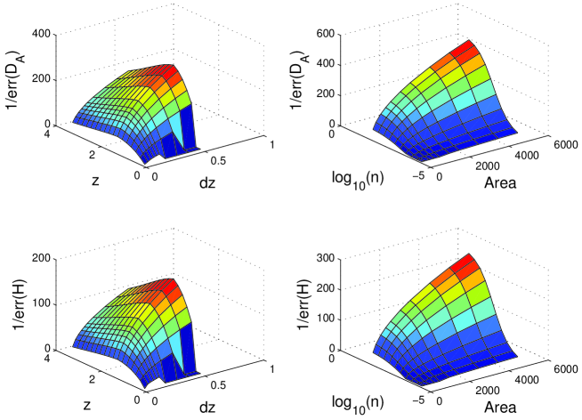
Figure 6: Dependence of the fitting formulae accuracies for spectroscopic surveys on pairs of survey parameters. For the left-hand plots we vary $z$ and $\delta z$, fixing $A=2$ and $n=5.1$. For the right-hand plots we vary $A$ and $n$, fixing $z=1$ and $\delta z=0.5$. The accuracy is plotted as $1/y$.

Figure 7: Tangential and radial baryon oscillation accuracies for spectroscopic redshift surveys as a function of survey area. We illustrate cases corresponding to the redshift windows that are naturally probed by optical spectrographs, $0.5<z<1.3$ and $2.5<z<3.5$. We have assumed a sufficient number density of galaxies that shot noise is unimportant. A reference line Accuracy $\propto$ Area^-1/2 is plotted. The dependence of accuracy on area becomes steeper for small areas because the baryon oscillations are no longer being adequately resolved by the data.

Figure 8: The tangential baryon oscillation accuracy for spectroscopic redshift surveys as a function of survey area for a series of redshift slices of width $0.2$. We have assumed a sufficient number density of galaxies that shot noise is unimportant. A reference line Accuracy $\propto$ Area^-1/2 is plotted. The dependence of accuracy on area becomes steeper for small areas because the baryon oscillations are no longer being adequately resolved by the data.

Figure 9: The same as Figure 8, plotting the radial baryon oscillation accuracy.

Figure 10: The tangential baryon oscillation accuracy for photometric redshift surveys as a function of survey area for a series of redshift slices of width $0.5$. We have assumed a photometric redshift error $\sigma_{0}=0.03$ and a sufficient number density of galaxies that shot noise is unimportant. A reference line Accuracy $\propto$ Area^-1/2 is plotted. The dependence of accuracy on area becomes steeper for small areas because the baryon oscillations are no longer being adequately resolved by the data.

Comparing the predictions of the fitting formulae with results from the full Monte Carlo method of BG03 (e.g. Glazebrook & Blake 2005, Table 1) we find that the mean difference is about $5\%$ of $y$ and the standard deviation of the difference is roughly $10\%$ of $y$. We can also compare the fitting formulae prediction with the accuracy of measurement of the acoustic scale by the SDSS LRG sample (Eisenstein et al. 2005). This survey covers sky area $3816$ deg² and redshift range $0.16<z<0.47$ ($V=0.72\,h^{-3}$ Gpc³). The galaxy number density varies with redshift, but we take an effective value $n_{\rm eff}=10^{-4}\,h^{3}$ Mpc^-3 and a galaxy bias corresponding to $\sigma_{8}=1.8$ (Eisenstein et al. 2005). The fitting formulae predict measurement accuracies of $6.4\%$ ($8.5\%$) in the tangential (radial) direction, using just the oscillatory information. Eisenstein et al. determined a $4\%$ measurement of the acoustic scale when the clustering pattern was averaged over angles, using the full information contained in the shape. Our combined tangential and radial measurements suggest an overall accuracy of about $5\%$ from just the oscillatory component, which appears broadly consistent.

5 Changing the cosmological parameters

These fitting formula coefficients have been derived from a grid of simulated surveys assuming a fiducial $\Lambda$CDM cosmology. However, the scaling arguments presented in Section 3 apply more generally. As a result, it is a good approximation to use the fitting formula of equation 6 for a range of cosmological parameters, if we compute the volume $V$, linear growth factor $D(z)$ and (where applicable) the radial position error $\sigma_{r}$ using the new set of parameters. The coefficients $x_{0}$, $V_{0}$, $\sigma_{r,0}$ and $D(z_{0})$ should remain unaltered at their $\Lambda$CDM calibrations. However, two further changes are required:

• The amplitude and shape of the input power spectrum $P$ depend on the cosmological parameters. Our technique is largely insensitive to these dependences because we divide out the overall power spectrum shape before fitting the baryon oscillations. However, the balance between cosmic variance and shot noise will be affected (i.e. the value of $nP$ in equation 3). For a new set of parameters, the coefficient $n_{\rm eff}$ should be scaled inversely with the characteristic power spectrum amplitude for the scales of interest, relative to its value in the fiducial case.

• We should re-estimate the cut-off redshift $z_{\rm m}$ at which all of the high-amplitude acoustic peaks become visible: the location of the non-linear transition scale at a given redshift depends on the growth of density perturbations, which is determined by the cosmological parameters.

6 Sparse-sampling strategies

Thus far, our formulae refer to surveys covering a fully contiguous sky area. However, the optimal strategy for measuring acoustic oscillations given a fixed observing time may not be to survey a contiguous area, but rather to sparsely-sample a larger area: gathering a larger density-of-states in Fourier space at the expense of an increased convolution of the input power spectrum (i.e. more smoothing of the acoustic oscillations) and increased correlations between adjacent Fourier bins (i.e. less statistical significance for an observed peak or trough in power). In practice, sparse-sampling could be achieved by a non-contiguous pattern of telescope pointing centres or, for a wide-field multi-object spectrograph, by distributing the fibres non-uniformly across the field-of-view.

In the first approximation, the effectiveness of a sparse-sampling strategy depends on the angular size $\theta$ of the observed survey patches (e.g. the field-of-view of the optical spectrograph) compared to the angular scale of the baryonic features in the power spectrum $\sim s/r(z)=2.6$ deg at $z=1$. If $\theta\sim 1$ deg then $W_{k}$ will contain structure on scales similar to the acoustic preferred scale, and an unacceptable degree of convolution will result. If $\theta\ll 1$ deg, then a sparse-sampling strategy will usually be preferred.

Figure 11: Effective area gain for a series of sparsely-sampled survey strategies at $z=1$, varying the filling factor $f$ of equation 10 and the survey patch size $\theta$. The area gains are evaluated using equation 12 and are compared with the simple increase in survey performance neglecting the effects of convolution and mode correlations (the dashed line). The cases analyzed are indicated by the solid circles.

We investigated this trade-off by simulating a series of sparse-sampling strategies with $\theta=2,5,10,30$ arcmin, considering spectroscopic redshift surveys only, and measuring the power spectrum in angle-averaged bins of constant wavenumber $k=\sqrt{k_{x}^{2}+k_{y}^{2}+k_{z}^{2}}$. For each value of $\theta$ we considered a series of survey ‘filling factors’ $1/f$ such that

$$f=\frac{{\rm Sparsely\,\,sampled\,\,area}}{{\rm Observed\,\,area}}$$ (10)

For the purposes of this simple investigation we assumed that the survey window function was a regular grid of square patches of size $\theta\times\theta$ (we note that other sampling strategies may be preferred, such as a random distribution of pointings or a logarithmic spiral). For each $(\theta,f)$ we determined an ‘effective area gain’ for the sparsely-sampled survey, by which we should multiply our observed (sparsely-sampled) area to produce the approximate input to the baryon oscillation fitting formulae.

The Fourier transform grid required to analyze a volume large enough to ensure a high-accuracy measurement of the baryon oscillations, whilst maintaining a resolution several times better than the sparse sampling scale of a few arcmin, is prohibitively large. Therefore we adopted a different approach, estimating the effective area gain by quantifying three competing effects:

• The average decrease in the amplitude $A$ of the acoustic oscillations due to convolution with the window function.

• The average decrease in the power spectrum error $\sigma$ in each Fourier bin (i.e. the diagonal elements of the covariance matrix) due to the increased number of Fourier modes analyzed.

• The increased correlation of each Fourier bin with its neighbours, defined by quantifying an ‘effective number of independent modes’ $m_{i}$ for each bin $i$ using the covariance matrix $C_{ij}$ of equation 1. For a uniform survey window function in a cuboid, $m_{i}=1/(\delta P_{i})^{2}=(P+\frac{1}{n})^{2}/C_{ii}$, where $P$ is the power spectrum amplitude in bin $i$. For a general window function we defined:

  $$m_{i}=\frac{(P+\frac{1}{n})^{2}}{\sum_{j}C_{ij}}$$ (11)

  such that the off-diagonal covariance matrix elements decrease the independence of the bins. We take the sum over $j$ up to the non-linear transition scale, and then define the average across the bins, $m=\overline{m_{i}}$.

We initially measured these quantities for a fiducial contiguous ($f=1$) survey of $100$ deg² spanning redshift range $0.75<z<1.25$. We then repeated our analysis for each pair of values of $(\theta,f)$ defining in each case

$${\rm Effective\,\,area\,\,gain}=\left(\frac{A/\sigma}{A_{0}/\sigma_{0}}\right)^{2}\frac{m}{m_{0}}$$ (12)

where the subscript ‘0’ indicates values for the fiducial survey. The relative powers of the quantities are chosen in accordance with their scaling with the number of Fourier modes $m$: Area $\propto m$ and $\sigma\propto 1/\sqrt{m}$. For the cases with small values of $\theta$, the convolution involves small-scale power from the non-linear clustering regime, thus we modified our input linear power spectrum using the non-linear prescription of Peacock & Dodds (1994).

The results are displayed in Figure 11. As expected, large survey patches $\theta\ga 30$ arcmin do not favour sparse-sampling strategies because of the consequent serious smoothing of the acoustic oscillations. If $\theta\la 10$ arcmin then sparse-sampling strategies are preferred, although we note that the resulting performance plotted in Figure 11, which includes the window function effects, is not as good as that which would be inferred by using the entire ‘sparsely-sampled area’ as the input area in the fitting formula, thus neglecting the window function effects (as indicated by the ‘simple area gain’ line plotted in Figure 11). We emphasize that our calculations here are only a first approximation and this is a subject requiring further study.

7 Summary

We have developed a fitting formula for the accuracy with which the characteristic baryon oscillation scale may be extracted from future spectroscopic and photometric redshift surveys in the tangential and radial directions, using heuristic scaling arguments calibrated using an accelerated version of the ‘model-independent’ method of Blake & Glazebrook (2003). The formula is given in equations 6 to 9 with the values of the parameters listed in Table 1, and reproduces the simulation results with a fractional scatter of $7\%$ ($10\%$) in the tangential (radial) direction, over a wide grid of survey configurations. Simple modifications allow the fitting formula to be applied for a range of cosmological parameters. We have also investigated how a simple sparse-sampling strategy may be used to enhance the effective survey area if the sampling scale $\theta$ is much smaller than the characteristic angular acoustic scale ($\theta\ll 1$ deg). This may be implemented for a wide-field multi-object spectrograph by clustering the fibres in the field-of-view.

References

- [1] Amendola L., Quercellini C., Giallongo E., 2005, MNRAS, 357, 429
- [2] Angulo R., Baugh C.M., Frenk C.S., Bower R.G., Jenkins A., Morris S.L., 2005, MNRAS, 362L, 25
- [3] Bassett B.A., 2005, PhRvD, 71, 3517
- [4] Bassett B.A., Parkinson D., Nichol R.C., 2005, ApJ, 626, 1
- [5] Bernstein G., 2005, ApJ, submitted (astro-ph/0503276)
- [6] Blake C.A., Bridle S.L., 2005, MNRAS, in press (astro-ph/0411713)
- [7] Blake C.A., Glazebrook K., 2003, ApJ, 594, 665
- [8] Carroll S.M., Press W.H., Turner E.L., 1992, ARA&A, 30, 499
- [9] Cole S. et al., 2005, MNRAS, 362, 505
- [10] Cooray A., Hu W., Huterer D., Joffre M., 2001, ApJ, 557L, 7
- [11] Eisenstein D.J., Hu W., 1998, ApJ, 496, 605
- [12] Eisenstein D.J., 2002, ‘Large-scale structure and future surveys’ in ‘Next Generation Wide-Field Multi-Object Spectroscopy’, ASP Conference Series vol. 280, ed. M.Brown & A.Dey (astro-ph/0301623)
- [13] Eisenstein D.J. et al., 2005, ApJ, in press (astro-ph/0501171)
- [14] Feldman H.A., Kaiser N., Peacock J.A., 1994, ApJ, 426, 23
- [15] Glazebrook K., Blake C., 2005, ApJ, 631, 1
- [16] Hu W., Haiman Z., 2003, Phys. Rev. D, 68, 063004
- [17] Huetsi G., 2005, A&A, submitted (astro-ph/0505441)
- [18] Lahav O. et al., 2002, MNRAS, 333, 961
- [19] Linder E.V., 2003, Phys. Rev. D, 68, 083504
- [20] Meiksin A., White M., Peacock J.A., 1999, MNRAS, 304, 851
- [21] Peacock J.A., Dodds S.J., 1994, MNRAS, 267, 1020
- [22] Seo H.-J., Eisenstein D.J., 2003, ApJ, 598, 720
- [23] Seo H.-J., Eisenstein D.J., 2005, ApJ, in press (astro-ph/0507338)
- [24] Springel V. et al., 2005, Nature, 435, 629
- [25] Tadros H., Efstathiou G.P., 1996, MNRAS, 282, 1381
- [26] Tegmark M., 1997, PRL, 79, 3806
- [27] White M., 2005, Astroparticle Physics, in press (astro-ph/0507307)
- [28] Yamamoto K., Bassett B.A., Nishioka H., 2005, PRL, 94, 51301