Physical implication of the KRL pulse function of gamma-ray bursts

Abstract

Kocevski, Ryde & Liang (2003, hereafter Paper I) proposed a semi-empirical function (the KRL function) of gamma-ray burst (GRB) pulses, which could well describe those pulses comprising a fast rise and an exponential decay (FRED) phases. Meanwhile, a theoretical model which could give rise to this kind of pulse based on the Doppler effect of the expanding fireball surface was put froward in details in Qin (2002) and Qin et al. (2004, hereafter Paper II). To provide a physical explanation to the parameters of the KRL function, we try to fit light curves of the Doppler model (Qin 2002; Paper II) with the KRL function so that parameters in both models can be directly related. We pay our attention only to single GRB pulses whose profiles are that of FRED and hence employ the sample presented in Paper I (the KRL sample) to study this issue. We find from our analysis that, for light curves, which arise from exponential rise and exponential decay local pulses, of the Doppler model, the ratio of the rise index $r$ to the decay index $d$, derived when fitted by the KRL function, increases quickly first, and then keeps nearly invariant with the relative width (relative to the timescale of the initial fireball radius $R_{c}/c$) of local pulses when the width exceeds 2 (the relative width is dimensionless). The rise and decay times of pulses are found to be related with the Lorentz factor by a power law, where the power law index associated with the rise time is less than that of the decay one and both of them are close to -2. In addition, the mean asymmetry shows a slightly trend of decreasing with lorentz factors. In plots of decay indexes versus asymmetry, there is a descending phase and after the phase there is a rising portion. We find that these long GRBs of the KRL sample are mainly associated with those light curves arising from co-moving pulses with the relative width being larger than 0.1. Shown in our analysis, the effect of the co-moving pulse shape on the KRL function parameters of the resulting pulses is considerable and can be distinguished by the decay index $d$ when the relative co-moving pulse width is less than 2 (when the relative width is larger than 2, it would be difficult to discern the difference in the resulting pulse shapes).

1 Introduction

Light curves of gamma-ray bursts (GRBs) exhibit very complex and distinct morphologies, without any systematic temporal features (Fishman & Meegan 1995). A single spectrum, generally the Band function spectrum, seems to be a universal characteristic of GRBs (Piran et al. 1997). The highly variable temporal structure of GRBs may provide the clue to disclose the puzzle about the spectrum observed (Sari et al. 1997). It was previously found that some individual peaks decay more gradually than they rise (e.g. Fishman et al., 1994; Fenimore E. E., 1999). Many GRBs can well be decomposed into fundamental pulses (Norris et al. 1996; Lee, Bloom, & Petrosian 2000a, 2000b), which comprise a fast rise and an exponential decay (FRED) phases in general. The pulse-shape light curves as the elementary events of GRBs probably provide the intrinsical information. Time asymmetry in GRB light curves has been discussed by several authors (see Barat et al. 1984; Norris et al. 1986; Kouveliotou et al. 1992; Link, Epstein, & Priedhorsky 1993; Nemiroff et al. 1994). The rise time ($t_{r}$), decay time ($t_{d}$), and full width at half maximum ($FWHM$) are the main factors concerned (McBreen et al. 2002; Ryde et al. 2003; Kocevski, Ryde & Liang 2003, hereafter Paper I). Norris et al. (1996) utilized a single flexible empirical function to represent pulses in long bright GRBs, and found the ratio of rise-to-decay times of pulses to be unity or less. Shown in Ryde & Svensson (2000, 2002) are some other fitting profiles.

To fully model the FRED light curves or individual pulse shapes, Kocevski et al. (2003) (Paper I) put forward an empirical function (the KRL function) described by

$$F(t)={F_{m}}(\frac{t}{t_{m}})^{r}[\frac{d}{d+r}+\frac{r}{d+r}(\frac{t}{t_{m}})^{(r+1)}]^{-\frac{r+d}{r+1}},$$ (1)

where $t_{m}$ is the time of the maximum energy flux, $F_{m}$, of the pulse. The shapes of single GRB pulses are confined by the two parameters $r$ and $d$. It is a very functional and flexible model based on the physical first principle and the well-established empirical correlation between $E_{p}$ and flux. This function could be adopted to characterize some GRB pulses such as FRED light curves. However, what can parameters $r$ and $d$ reveal if the FRED pulses described by the KRL function arise from fireball sources?

Recently, a theoretical pulse model (called the Doppler model) was proposed (see section 2 below) to relate the observed characteristics of GRB pulses with parameters of the intrinsic radiation in the framework of fireballs, where the Doppler effect associated with the expanding fireball surface is the key factor to be concerned (Qin 2002; Qin et al. 2004, hereafter Paper II). Illustrated in this model, the profile of an observed pulse would mainly be determined by the intensity of co-moving pulses, $\widetilde{I}(\tau_{\theta})$ (see Paper II). It was revealed that most of the resulting pulses possess a characteristic of FRED, even though the co-moving pulses concerned are diverse significantly.

Hinted by the common FRED feature shown in the two models, a primary goal of this paper is born. We want to know how parameters $r$ and $d$ would be associated with intrinsic quantities such as the Lorentz factor $\Gamma$ and the co-moving pulse width $\Delta\tau_{\theta}$ (see below), once co-moving pulses are provided (see Paper II). Some prevenient investigations did’t take into account the influence of co-moving pulses on the observed light curve (see, e.g., Ryde 2004). However, as mentioned above, it was shown in the Doppler model that the observed pulse shape (especially its peakedness) is mainly associated with the co-moving pulse shape and width.

In the following, we will investigate the impacts of exponential rise and exponential decay co-moving pulses on the observed light curve in detail. In section 2 we will introduce formulas of the Doppler model to describe the observed FRED pulses. In section 3, we will give a reason for choosing the types of co-moving pulse and will simulate a lot of resulting pulses and then will fit them with equation (1), and in doing so, some parameters associated with the observed light curve will be presented. In section 4, we will contrast our results with those derived from observation. Our results will be discussed and summarized in section 5.

2 Formulas of the Doppler model employed in this paper

We list in this section basic formulas, which were derived and presented in Paper II, of the Doppler model so that it would be convenient for us to employ or refer to them in the following analysis.

Adopting the same symbols assigned and used in Paper II, the count rate equation derived from the expected flux emitted from an expanding fireball surface is expressed as (see Paper II)

$$C(\tau)=C_{0}\frac{\int\limits_{\widetilde{\tau}_{\theta,min}}^{\widetilde{\tau}_{\theta,max}}\widetilde{I}(\tau_{\theta})(1+\beta\tau_{\theta})^{2}(1-\tau+\tau_{\theta})d\tau_{\theta}\int\limits_{\nu_{1}}^{\nu_{2}}\frac{g_{0,\nu}(\nu_{0,\theta})}{\nu}d\nu}{\Gamma^{3}(1-\beta)^{2}(1+\frac{\beta}{1-\beta}\tau)^{2}},$$ (2)

where $\beta=\sqrt{\Gamma^{2}-1}/\Gamma$, $\Gamma$ is the Lorentz factor, $C_{0}$ is a constant which includes the luminosity distance $D$ between the fireball and the observer and other factors (see Paper II), $\widetilde{I}(\tau_{\theta})$ represents the development of the intensity of the co-moving emission (in this paper, the co-moving pulse), $g_{0,\nu}(\nu_{0,\theta})$ describes the rest-frame radiation mechanism, and $\nu_{0,\theta}$ is the rest frame emission frequency which is related with the observed frequency $\nu$ by the Doppler effect. In equation (2), the count rate concerned is defined within an energy channel of [$\nu_{1}$, $\nu_{2}$]. As shown in Paper II, letter “$t$” denotes an absolute value of time which is normally defined (it is always in units of $s$), and the Greek letter “$\tau$” represents a relative time scale (in units of 1) corresponding to “$t$”. The two types of quantity are related by (see Paper II)

$$\tau\equiv\frac{t-t_{c}-D/c+R_{c}/c}{R_{c}/c},$$ (3)

$$\tau_{\theta}\equiv\frac{t_{\theta}-t_{c}}{R_{c}/c},$$ (4)

$$\tau_{\theta,min}\equiv\frac{t_{\theta,min}-t_{c}}{R_{c}/c},$$ (5)

and

$$\tau_{\theta,max}\equiv\frac{t_{\theta,max}-t_{c}}{R_{c}/c},$$ (6)

where $t_{c}$ and $R_{c}$ are constants, and we assign $t_{\theta,min}\leq t_{\theta}\leq t_{\theta,max}$ (and hence $\tau_{\theta,min}\leq\tau_{\theta}\leq\tau_{\theta,max}$). The limits of the integral of $\tau_{\theta}$ in formula (2) are $\widetilde{\tau}_{\theta,min}=max\{\tau_{\theta,min},(\tau-1+\cos\theta_{max})/(1-\beta\cos\theta_{max})\}$ and $\widetilde{\tau}_{\theta,max}=min\{\tau_{\theta,max},(\tau-1+\cos\theta_{min})(1-\beta\cos\theta_{min})\}$, where $\theta_{min}$ and $\theta_{max}$ are the lower and upper limits of angle $\theta$, respectively (see Paper II). One could find from these definitions that $\tau$ and $\tau_{\theta}$ are dimensionless quantities.

Note that, the value of $t_{c}$ could be arbitrarily chosen (it depends on the time we assign to that moment). For the sake of simplicity, we take

$$t_{c}=(R_{c}-D)/c$$ (7)

in the following analysis, where $R_{c}$ is the initial radius of the fireball (measured at time $t_{c}$). In this way, one gets

$$\tau=\frac{t}{R_{c}/c}.$$ (8)

Substituting this relation into formula (2), the count rate as a function of observation time $t$ could then be plainly illustrated, so long as $R_{c}$ is available (or assumed).

In this paper, we take the generally adopted spectral form proposed by Band et al. (1993), the so-called Band function

$$$$g_{0,\nu,B}(\nu_{0,\theta})=\left\{\begin{array}[]{cc}(\frac{\nu_{0,\theta}}{\nu_{0,p}})^{1+\alpha_{0}}exp[-(2+\alpha_{0})\frac{\nu_{0,\theta}}{\nu_{0,p}}],&\ \ (\frac{\nu_{0,\theta}}{\nu_{0,p}}\leq\frac{\alpha_{0}-\beta_{0}}{2+\alpha_{0}})\\ (\frac{\alpha_{0}-\beta_{0}}{2+\alpha_{0}})^{\alpha_{0}-\beta_{0}}exp(\beta_{0}-\alpha_{0})(\frac{\nu_{0,\theta}}{\nu_{0,p}})^{1+\beta_{0}}&\ \ ({\rm}\frac{\nu_{0,\theta}}{\nu_{0,p}}>\frac{\alpha_{0}-\beta_{0}}{2+\alpha_{0}})\\ \end{array}\right.$$,$$ (9)

as the rest frame spectrum $g_{0,\nu}(\nu_{0,\theta})$.

One might observe that the profile of the KRL function are determined by parameters $r$ and $d$. However, in the Doppler model, the characteristics of an observed pulse would be obviously influenced by the Lorentz factor and the co-moving intensity of radiation (see Paper II). Thus, by fitting light curves of formula (2) with function (1), one might be able to tell how parameters $r$ and $d$ and various widths of the KRL function are related with the Lorentz factor and co-moving pulses, assuming that the sources observed are undergoing a fireball stage.

3 General analysis on the pulses of fireball sources

In this section, we study the light curve of formula (2) in a particular case: the adopted co-moving pulse is an exponential rise and an exponential decay one. Various sets of parameters $r$ and $d$ of the KRL function would be obtained when fitting light curves of formula (2) associated with different Lorentz factors and different widths of the co-moving pulse with equation (1). In this process, we consider the radiation from the whole spherical surface of the fireball, although the contribution from the area of $\theta>1/\Gamma$ is insignificant. (Impacts of different emission areas in the fireball surface on the resulting pulses were shown in Paper II.) Thus, we adopt $\theta_{min}=0$ and $\theta_{max}=\pi/2$. Not losing the generality, we assign $C_{0}=1$. In addition, we take $\nu_{1}=50\nu_{0,p}$ and $\nu_{2}=100\nu_{0,p}$, where $\nu_{0,p}$ is the break frequency of the rest frame Band function spectrum, so that when assigning $\nu_{0,p}=1keVh^{-1}$ the energy range would correspond to the second channel of BATSE.

It is supposed that a very violent collision of two shells gives rise to the observed GRB pulse behavior, and the increase (or decrease) of co-moving emission is proportional to the total radiation in the rise (or decay) phase of the co-moving pulse, namely

$$$$dI(\tau_{\theta})=\left\{\begin{array}[]{cc}\frac{1}{\sigma_{r}}I(\tau_{\theta})d\tau_{\theta}&\ \ (in\ the\ rise\ phase)\\ -\frac{1}{\sigma_{d}}I(\tau_{\theta})d\tau_{\theta}&\ \ (in\ the\ decay\ phase)\\ \end{array}\right.$$,$$ (10)

where $\sigma_{r}$ and $\sigma_{d}$ are two positive constants. Integrating this equation leads to

$$$$I(\tau_{\theta})=I_{0}\left\{\begin{array}[]{cc}exp[(\tau_{\theta}-\tau_{\theta,0})/\sigma_{r}]&\ \ (\tau_{\theta,min}\leq\tau_{\theta}\leq\tau_{\theta,0})\\ exp[-(\tau_{\theta}-\tau_{\theta,0})/\sigma_{d}]&\ \ (\tau_{\theta,0}<\tau_{\theta}\leq\tau_{\theta,max})\\ \end{array}\right.$$,$$ (11)

where $I_{0}$ and $\tau_{\theta,0}$ are the integral constants. Associated with the well-known mechanisms, the rising part of this co-moving pulse might connect to the shell crossing time and the decay portion might relate to the cooling time. (It is interesting that a pulse form with an exponential rise and an exponential decay phases was previously adopted as an empirical function to describe some observed GRB pulses by Norris et al. 1996). The spiky form of this co-moving pulse implies that the physical interaction processes of shells are greatly impetuous and rapid.

In the process of the shell collision, two intrinsic timescales, the cooling timescale of electrons and the shell crossing timescale, should be considered simultaneously, and they together would cause the width of the co-moving pulse. In terms of the Doppler model, co-moving pulses would be significantly altered by the expanding fireball surface and then would lead to the observed forms of pulses (see Paper II). An alternative interpretation to this is that the two timescales together with the curvature timescale which is due to the relativistic kinematics of expanding shell would give rise to the observed pulses. In many cases, the curvature time and the shell crossing time dominate over the cooling time (See, Ryde et al. 2003). Spada et al. (2000) suggested that this case will occur at a distance $R<5\times 10^{14}cm$, but for larger radii the radiative cooling time will become the dominant contribution to the pulse duration (in the first case the cooling timescale would be relatively small while in the last case it would be relatively large).

For convenience, the width of co-moving pulse (11) is defined as

$$\Delta\tau_{\theta}=\tau_{\theta,max}-\tau_{\theta,min}.$$ (12)

Note that the quantity $\Delta\tau_{\theta}$ determined by eqs. (5) and (6) is also dimensionless. In the following analysis we assign $\tau_{\theta,min}=-\sigma_{r}$, $\tau_{\theta,max}=\sigma_{d}$ and $\tau_{\theta,0}=0$ in order to check whether the ratio of the rise time to the decay time of co-moving pulses can influence the observed light curves. Here we consider two kinds of spiky co-moving pulses. One concerns $\sigma_{r}=\sigma_{d}$ (case 1) and the other is associated with $\sigma_{r}=4\sigma_{d}$ (case 2).

3.1 In the case of $\sigma_{r}=\sigma_{d}$

Here, we consider co-moving pulse (11) with $\sigma_{r}=\sigma_{d}$, which implies that the cooling time and the shell crossing time are comparable.

3.1.1 Impact of the co-moving pulse width

To investigate how parameters $r$ and $d$ are related with the co-moving pulse width, we calculate various light curves of formula (2), arising from co-moving pulse (11) with $\Delta\tau_{\theta}$ = 0.001, 0.002, 0.005, 0.01, 0.02, 0.05, 0.1, 0.2, 0.5, 1, 2, 5, 10 respectively (The reason to choose these values is discussed in Appendix B.), and then fit them with the KRL function. For the rest frame Band function spectrum we take $\alpha_{0}=-1$ and $\beta_{0}=-2.25$, and for the Lorentz factor we consider $\Gamma$ = 2, 5, 10, 100, 1000, and 10000. Parameters $r$ and $d$ are directly obtained from the fit. The rising width $t_{r}$ and the decaying width $t_{d}$ of the observed pulse would be obtained from equation (1) when the fitting parameters are applied. (Note that, quantities $t_{r}$ and $t_{d}$ are consistent with those denoted respectively in Paper I.) We define the asymmetry of the observed pulse as $t_{r}/t_{d}$, the ratio of the rise fraction timescale of the pulse to the decay fraction timescale.

(i) Relations between these parameters ($r$, $d$, $r/d$, $t_{r}$, $t_{d}$, $t_{r}/t_{d}$) and the co-moving pulse width $\Delta\tau_{\theta}$ are shown in Fig. 1. Shown in panel (a), there lie minimums of $d$ between $\Delta\tau_{\theta}=0.03$ and 0.1. From panels (a), (b), (c) and (f), we find that $d$, $r$, $r/d$ and $t_{r}/t_{d}$ are independent of $\Delta\tau_{\theta}$ when $\Delta\tau_{\theta}$ is larger than 2. In terms of the KRL function, the result suggests that profiles of the observed light curves would not be distinguishable when the width of co-moving pulses is large enough (say $\Delta\tau_{\theta}>2$), which is in agreement with what revealed in Paper II (see Paper II Fig. 3). According to equation (4), a large value of $\Delta\tau_{\theta}$ suggests a relatively small value of the radius of the fireball, and this in turn indicates that the curvature timescale is relatively small. In this situation, it would be reasonable when the cooling time plus the shell-crossing time dominate far over the curvature timescale. However, as shown in panel (f), the pulse asymmetry would decease rapidly with the decreasing of the co-moving pulse width when $\Delta\tau_{\theta}<2$. Panels (d) and (e) indicate that $t_{r}$ increases with the increasing of $\Delta\tau_{\theta}$ at all time, while $t_{d}$ is sensitive to $\Delta\tau_{\theta}$ only when $\Delta\tau_{\theta}$ is large enough (say $\Delta\tau_{\theta}>0.1$). This must be due to the fact that when the curvature timescale dominates far over the two other timescales, the decay phase of the light curve would be determined by the curvature effect and its profile would remain unchanged when $\Delta\tau_{\theta}<0.1$(approaching the so-called standard form defined in Paper II; see also Paper II Fig. 3). A contrast between panels (c) and (f) suggests that the ratio of $r$ to $d$ doesn’t adapt to characterize the asymmetry of the observed pulses.

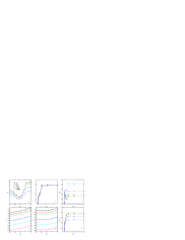
Figure 1: Relations of parameters ($d$, $r$, $t_{r}$, $t_{d}$, $r/d$, and $t_{r}/t_{d}$) of the observed light curves and the co-moving pulse width ($\Delta\tau_{\theta}$) for different lorentz factors ($\Gamma$ = 2, 5, 10, 100, 1000, 10000) respectively. Symbols corresponding to different values of $\Gamma$ are displayed in panel (a).

(ii) Displayed in Fig. 2 are the relations between parameters $d$, $r$, $r/d$, $t_{r}/t_{d}$, $FWHM$, and $t_{r}/FWHM$. Shown in panel (a), the smallest value of index $d$ could be detected in the range of $0.5<r<1$. Panels (b) and (f) also demonstrate the existence of a minimum of $d$, with the minimum corresponding to smaller values of $t_{r}/t_{d}$ and $t_{r}/FWHM$ when the Lorentz factor becomes larger. One finds from panel (e) that, for a given Lorentz factor, the pulse asymmetry is very sensitive to the co-moving pulse width when the latter is very small, and when the latter becomes large enough, the asymmetry would become invariant. This is in good agreement with what illustrated above. In addition, panel (e) shows that the larger the Lorentz factor the narrower the pulse observed, which is in consistent with what previously known (see, e.g., Fenimore et al. 1993).

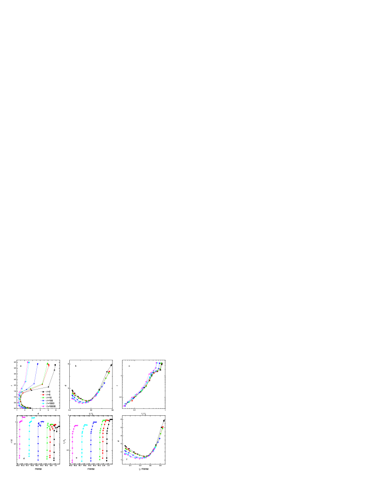
Figure 2: Relations between parameters $d$, $r$, $r/d$, $t_{r}/t_{d}$, $FWHM$, and $t_{r}/FWHM$, where we adopt $\Gamma$ = 2, 5, 10, 100, 1000, 10000 respectively. Symbols associated with different Lorentz factors are denoted in panel (a).

We find that characteristics of the relationships displayed in Figs. 1 and 2 are the same for different Lorentz factors.

3.1.2 Impact of the Lorentz factor

Here, we study how parameters $d$, $r$, $r/d$, $t_{r}$, $t_{d}$ and $t_{r}/t_{d}$ are related with $\Gamma$ when different values of $\Delta\tau_{\theta}$ are adopted. We take $\Gamma$ = 2, 5, 10, 70, 100, 150, 200, 500, 1000, 10000 respectively. Five typical values of the co-moving pulse widths, $\Delta\tau_{\theta}$ = 0.001, 0.01, 0.1, 1, and 10, are adopted. The indexes of the rest frame Band function spectrum are the same as those adopted above. In the same way, light curves of (2) associated with various sets of these intrinsic parameters are calculated and then are fitted with equation (1).

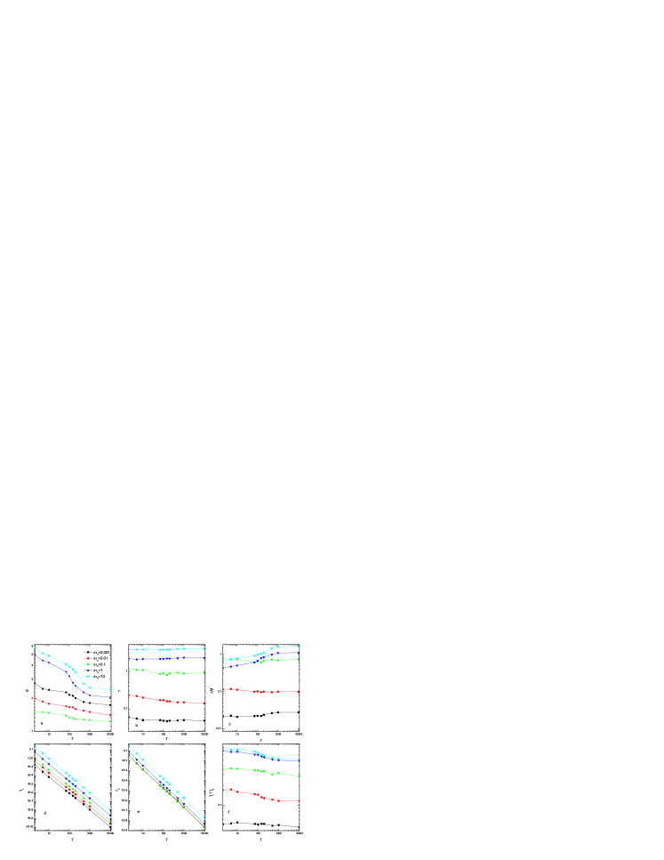
Figure 3: Relations of parameters ($d$, $r$, $t_{r}$, $t_{d}$, $r/d$, $t_{r}/t_{d}$) of the observed light curves and the Lorentz factor $\Gamma$ associated with different values of the co-moving pulse width ($\Delta\tau_{\theta}$ = 0.001, 0.01, 0.1, 1, 10) respectively. Symbols are denoted in panel (a).

Shown in Fig. 3 are the relations of parameters of the KRL function associated with the observed light curves and the Lorentz factor. As shown in panel (f), the effects of $\Gamma$ on the pulse asymmetry are negligible, although a weak anti-correlation between $t_{r}/t_{d}$ and $\Gamma$ is visible. The following relations could be concluded from panels (d) and (e):

$$t_{r}\propto\Gamma^{\alpha_{r}}$$ (13)

and

$$t_{d}\propto\Gamma^{\alpha_{d}}.$$ (14)

Values of $\alpha_{r}$ and $\alpha_{d}$ could be obtained by performing a linear fit to the logarithmic format data of the two panels. The results are listed in Table 1. The relation $\Delta\tau_{FWHM}\propto\Gamma^{-2}$ was obtained by Qin et al. (2004) (Paper II) when an extremely narrow co-moving pulse is concerned. The index of $-2$ is nothing but merely a result of time compression effect caused by the forward motion of the ejecta (see Appendix A). The values of $\alpha_{r}$ and $\alpha_{d}$ presented in Table 1 are close to $-2$, which must be due to the same time compression effect. Note that the observed timescale lasts a little longer (as the indexes are slightly larger than $-2$) than what the time compression effect suggests. This could be understood when one recalls that what we consider in this paper is a fireball surface rather than an ejecta moving towards the observer (in the latter case, $\theta=0$) and the emission of the surface lasts an interval of time (if the emission is extremely short, we come to Paper II equation [44]). Shown in Table 1 we observe that $\alpha_{d}$ is slightly larger than $\alpha_{r}$. This suggests that the rising part of the observed pulse is less affected by the fireball surface than the decay portion is (the less affected by the fireball surface the closer the index to $-2$).

Table 1: Power law indices $\alpha_{r}$ and $\alpha_{d}$ derived for cases 1 and 2

case	$\Delta\tau_{\theta}$	$\alpha_{r}$	$\chi^{2}/\nu$	$\alpha_{d}$	$\chi^{2}/\nu$
	0.001	-1.95	2.7	-1.92	3.1
	0.01	-1.98	3.0	-1.93	2.6
$\sigma_{r}=\sigma_{d}$	0.1	-1.97	2.7	-1.93	2.9
	1	-1.99	3.2	-1.94	2.8
	10	-1.99	3.0	-1.94	2.7
	0.001	-1.90	2.7	-1.87	2.8
	0.01	-1.91	2.9	-1.87	2.7
$\sigma_{r}=4\sigma_{d}$	0.1	-1.90	3.0	-1.87	2.8
	1	-1.94	2.9	-1.89	3.0
	10	-1.93	3.0	-1.88	3.0

(ii) Relations between parameters shown in Fig. 2, the characters of the observed light curves (ie., $d$, $r$, $r/d$, $t_{r}/t_{d}$, $FWHM$, and $t_{r}/FWHM$), are displayed in Fig. 4, where different data points correspond to different values of $\Gamma$ (data points associated with the same value of $\Delta\tau_{\theta}$ are denoted by the same symbol).

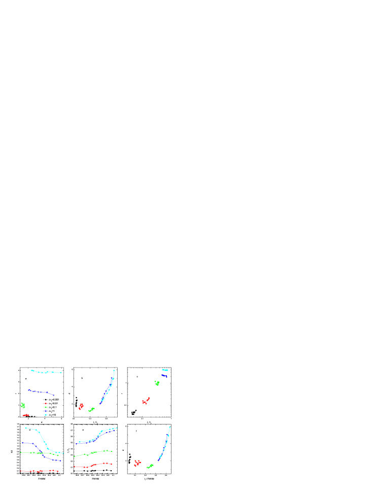
Figure 4: Relations between parameters of the observed light curves associated with $\Delta\tau_{\theta}$ = 0.001, 0.01, 0.1, 1, 10 respectively. Symbol are denoted in panel (a).

Panel (e) shows that, for very narrow co-moving pulses, asymmetry of the observed pulses would keep to be invariant with $FWHM$, while for wider co-moving pulses, the asymmetry would decrease first and then would keep to be invariant with the decreasing of $FWHM$ (here, since the co-moving pulse width is fixed, the decreasing of $FWHM$ would be caused by the increasing of the Lorentz factor). Panels (b), (c) and (f) are similar to the corresponding panels in Fig. 2. They implies that: (1) there is a correlation between parameters $d$ and $t_{r}/FWHM$ in $t_{r}/FWHM\geq 0.2$ (or $\Delta\tau_{\theta}\geq 0.1$) and an anti-correlation between the two quantities in $t_{r}/FWHM\leq 0.2$ (or $\Delta\tau_{\theta}\leq 0.1$) (see section 4 for a detailed discussion), no matter what the Lorentz factors are. (2) a power law relation probably exists between parameters $r$ and $t_{r}/t_{d}$. Let us assume

$$t_{r}/t_{d}\propto r^{\epsilon}.$$ (15)

Fitting the logarithmic format data with a linear function, we obtain $\epsilon=0.578$. It shows that index $r$ and the pulse asymmetry tie in, and the former can measure the latter as long as the co-moving pulse is known.

The result that the pulse asymmetry for long bursts will decrease as the $FWHM$ narrows supports previous conclusions found by Norris et al. (1996) (see also e.g. Reichart et al. 2001). As shown in Paper II, a small value of $FWHM$ could be caused by a small co-moving pulse width, or a small fireball radius, or a large Lorentz factor. Of the three factors, the third is the most sensitive one according to the Doppler model.

3.2 In the case of $\sigma_{r}=4\sigma_{d}$

Now we study the case of adopting co-moving pulse (11) with $\sigma_{r}=4\sigma_{d}$ (case 2), which corresponds to a relatively fast cooling timescale of electrons.

In order to find out whether there is any difference between the two cases, we perform the same analysis as that in case 1. The only difference in this analysis is that we replace $\sigma_{r}=\sigma_{d}$ with $\sigma_{r}=4\sigma_{d}$ for co-moving pulse (11). It is surprised that characteristics shown in the corresponding relations in the two cases are very similar. Conclusions drawn from case 1 holds in case 2. However, parameter $d$ shows a difference in the two cases, which is illustrated in Fig. 5 (presented in this figure is also the comparison between the values of $r$ for the two cases). To produce the data of this figure, we take $\Gamma=100$. As suggested by the figure, index $d$ is more sensitive to the co-moving pulse than $r$ is. This enables us to relate an observed pulse with the corresponding co-moving pulse by parameter $d$ so long as $\Delta\tau_{\theta}$ is smaller than 2. It suggests that a lager value of $d$ may correspond to a faster cooling process. Once $\Delta\tau_{\theta}$ becomes larger than 2, it would be difficult to discern different co-moving pulses from $d$.

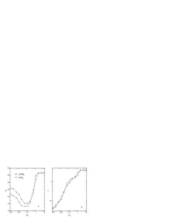
Figure 5: Relations between parameters ($d$ and $r$) of the observed light curve and the co-moving pulse width for cases 1 and 2. Here we take $\Gamma$ = 100. Relations associated with $d$ and $r$ are presented in panels (a) and (b), respectively. Symbols are denoted in panel (a).

The analysis shows that parameters $\alpha_{r}$ and $\alpha_{d}$ in case 2 are larger than those in case 1. This indicates that the influence of the co-moving pulse in case 2 on observations is greater than that in case 1.

In case 2, regarding relation (15) we get $\epsilon=0.464$ by a linear fit. It shows that the same conclusion obtained in case 1 holds in this case.

4 Comparison with the observed data

Let us contrast Fig. 4 panel (f) with Paper I Fig. 12 to provide a direct comparison between the observed data and the expectation of the Doppler model in the relationship between $d$ and $t_{r}/FWHM$. In Fig. 4 panel (f), data in the decaying portion of the relationship curve (the data associated with $\Delta\tau_{\theta}<0.1$) are defined as sample 1, while those in the rising portion (the data associated with $\Delta\tau_{\theta}\geq 0.1$) are called sample 2. The corresponding sets of data in case 2 are also called sample 1 (the data associated with $\Delta\tau_{\theta}<0.1$) and sample 2 (the data associated with $\Delta\tau_{\theta}\geq 0.1$) respectively. The data presented in Paper I include 77 individual pulses with time profiles longer than 2 seconds, which we define as sample 3.

One might observe that analysis performed in the previous sections is based on the concept of $\tau$ which is dimensionless. Relation between this quantity and the observed time $t$ is shown in equation (8). As $\tau$ is proportional to $t$, parameter $t_{r}/FWHM$ would be the same in both definitions. Fortunately, $d$ is dimensionless. We therefore can directly compare data of samples 1 and 2 with those of sample 3. Plots of $d$ vs. $t_{r}/FWHM$ for cases 1 and 2 together with the data of sample 3 are shown in Fig. 6 panels (a) and (b) respectively. Presented in the figure is also the division (at $t_{r}/FWHM\simeq 0.2$) between samples 1 and 2.

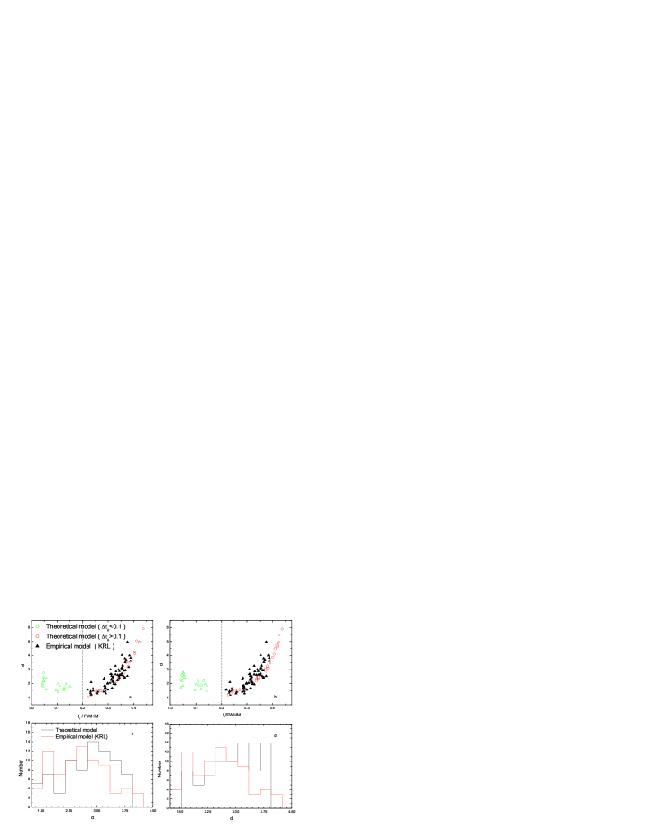
Figure 6: Comparison between sample 3 and samples 1 and 2 in the planes of $d$ vs. $t_{r}/FWHM$ and number vs. $d$, where 1) panel (a) is associated with case 1 while panel (b) corresponds to case 2. [Note that, data of samples 1 and 2 plotted in panel (a) are merely the replicate of Fig. 4 panel (f).] The vertical line denotes the position of $t_{r}/FWHM\simeq 0.2$ (or $\Delta\tau_{\theta}\simeq 0.1$) which divides data of sample 1 from those of sample 2. Symbols are denoted in panel (a). 2) Panels (c) and (d) shows distributions of index $d$ for case 1 and case 2 respectively. The assumed lognornmal distribution of $\Delta\tau_{\theta}$ [see eq.(16)] yields the theoretical $d$ distribution as the lorentz factor is taken one typical value, say, $\Gamma=100$. Same symbol meanings as in panel(c).

We find in surprise that sample 3 is well within the range of sample 2, while it is completely irrelevant to sample 1. In addition, sample 3 shows a positive correlation between $d$ and $t_{r}/FWHM$ just as what sample 2 shows. To investigate whether samples 2 and 3 have indeed the same distribution on a certain significance level, we take a general K-S test to the two-dimensional distributions of the two samples. We adopt the effective D definition of two-dimensional K-S statistic D as the average of two values obtained by above samples individually.(see, Press et al.(1992)) The K-S statistic and the indicated probability (significance level) are listed in Table 2.

Table 2: Parameters gained by two- and one-dimensional K-S test for respective cases 1 and 2

Panels	KS	Probability	Degrees of freedom
a	0.3075	0.0475	n1=30, n2=76
b	0.4145	0.0022	n1=30, n2=76
c	0.2237	0.0376	n1=n2=76
d	0.2895	0.0026	n1=n2=76

Above results in both case 1 and case 2 imply that sample 2 and sample 3 are not significantly different in terms of statistics. Based on the fact that sample 3 is composed of 77 individual pulses with durations longer than 2 seconds, we thus deduce that long GRBs could be mainly superposed by wider rest-frame radiation pulses with $\Delta\tau_{\theta}\geq 0.1$. Motivated by the viewpoint that the short bursts with $T_{90}<2.6s$ have different temporal behaviors compared with the long ones and they may actually constitute a different class of GRBs (e.g. Norris, Scargle, & Bonnell 2001), we suppose sample 1 with $\Delta\tau_{\theta}<0.1$ might hold the characteristic of short GRBs. The fact that sample 2 associated with $\Delta\tau_{\theta}\geq 0.1$ is consistent with sample 3 in distributions seems to demonstrate at least some of sources in sample 3 could be described by Qin’s theoretical model in a sense of practice.

To check if the distribution of index $d$ in sample 3 is indeed expectable, we plot the distribution of $d$ that is found from Fig. 1a for a assumed distribution of $\Delta\tau_{\theta}$. The rise times ($t_{r}$), fall times ($t_{d}$), FWHM, as well as the time intervals between pulses had been measured and found to be consistent with lognormal distributions for both short and long GRBs [McBreen et al. 2002]. Now, let us also consider Gaussian distribution of the logarithmic format of quantity $\Delta\tau_{\theta}$:

$$p(log\Delta\tau_{\theta})\propto\exp[-\frac{1}{2}(\frac{log(\Delta\tau_{\theta})+0.15}{0.85})^{2}],$$ (16)

So, many random values of $\Delta\tau_{\theta}$ could be yielded so long as the reasonable range of $\Delta\tau_{\theta}$ can well be determined. In Fig. 1a, suppose we take $\Gamma=100$, a correlation between $d$ and $\Delta\tau_{\theta}$ within the range of $0.1\leq\Delta\tau_{\theta}\leq 2$ (Note that, resulting pulses within this range are correlated with sample 3 and can then be distinguished with parameter $d$ in KRL function) offers us an opportunity to gain the index $d$ corresponding with $\Delta\tau_{\theta}$. Plots of distribution of $d$ for cases 1 and 2 together with the data of sample 3 are shown in Fig. 6 panels (c) and (d) respectively. Likewise, the K-S test to above distributions is also made to give the statistic and indicated probability listed in Table 2. We find the two distributions are not significantly different from viewpoint of statistics.

5 Conclusions and discussions

According to above-mentioned analyses, we can draw the underlying conclusions:

First, effects of different sorts of spikier co-moving pulses on the observed pulse shapes could be distinguished by shape parameter $d$ provided $\Delta\tau_{\theta}$ is less than 2 or so. However, parameter $r$ in KRL function and pulse asymmetry could be bound with the relationship $t_{r}/t_{d}\propto r^{\epsilon}$. Secondly, the asymmetry of observed pulses exhibits a slight trend of decrease with the increasing of $\Gamma$, whereas it increases quickly with the increasing of $\Delta\tau_{\theta}$ when $\Delta\tau_{\theta}\leq 2$, beyond this range, it will keep invariant with $\Delta\tau_{\theta}$. In observer framework, we find the asymmetry increase quickly first with $FWHM$ and then behaves nearly independent of $FWHM$ for an assumed $\Gamma$ or a lager $\Delta\tau_{\theta}$. Thirdly, two power law relations, $t_{r}\sim\Gamma^{\alpha_{r}}$ and $t_{d}\sim\Gamma^{\alpha_{d}}$ have been surprisingly found to show the width of observed pulse is highly sensitive to lorentz factors. Along with previous result (Paper II eq.[4]), we attribute these properties to the so-called time compression effect, which is purely kinematical and independent of physical mechanism, as long as the emission comes from an expanding fireball. Further, the difference of indexes $\alpha_{r}$ and $\alpha_{d}$ in case 1 from those in case 2 suggests that diverse intrinsic emission processes may cause distinct influences on observed profiles.

Following from the discussion in $\S 4$, for reasons not presently understood, the result that there is a decay portion (sample 1) in plot of $d$ vs. $t_{r}/FWHM$ which disappears in Kocevski’s plot (Paper I, Fig. 12) is rather surprising. We believe that there might be some bursts arising from short co-moving pulses associated with $\Delta\tau_{\theta}<0.1$ and their corresponding pulses would be observed if our sample is large enough, and in this case the corresponding data would be located within the descending portion in this plot. The two sub-classes of GRBs show completely different behaviors though they can be explained with the same emission mechanism, which in general being ascribed to synchro-Compton radiation via internal shocks, not the external shocks (see, Piran et al. 1997, Nakar et al. 2001 & McBreen et al. 2001, 2002). Based on this comprehension, we infer that the decay portion probably encompasses the short bursts or at least some of them.

As mentioned above, our whole investigations are built on the assumptions of the fireball-model and the isotropic radiation. Further, all the co-moving pulses concerned in this paper have a certain width, that is $\Delta\tau_{\theta}>0$. Previous studies on light curves of a co-moving $\delta$-function pulse (see, Paper II) found that this very narrow pulse will lead to a standard form light curve, which has only decay phase in the resulting pulses due to pure curvature effect. As it shows in Fig. 1 that the difference in contribution of $\Delta\tau_{\theta}$ to rise times and decay times of light curves is visible. This shows the rise phase of pulses as a result of the contribution of $\Delta\tau_{\theta}$ would reflect not only the energizing of the shell but also the radiative cooling of electrons, while the decay portion of the observed pulse could be fully characterized by all above-mentioned timescales (namely, curvature time , shell-crossing time and radiative cooling time). In the case of $\Delta\tau_{\theta}\gg 0.1$, the Doppler model is not the major contributor of the pulse shape and indeed the co-moving behavior could be important. The conclusion is just in excellent agreement with that of Spada et al.(2000)

By simulating many resulting pulses with several sorts of co-moving pulses, We find the resulting pulses modelled by Qin’s model are mainly determined by their corresponding co-moving forms and lorentz factors. Assuming one monotonic rise (or decay) function is selected to stand for the co-moving form, the resulting pulses will show concave (or convex) in phase of rise. In addition, we find the kurtosis especially the rise part of resulting pulses mainly originates from the spiky co-moving forms as long as $\Delta\tau_{\theta}$ is not very narrow enough, otherwise, these peaked resulting pulses will behave greatly similar to the so-called standard forms. In other cases, we can always achieve the flat-peaked resulting pulses provided that the decay phase of co-moving pulses is in existence.

From an viewpoint of observation, how to choose the co-moving pulse form for an observed GRB is an urgent issue. Within the range of $0.001\leq\Delta\tau_{\theta}<2$ (namely, 0.5 s $\leq$“t” $\leq$1000 s), the shape of resulting pulses could be well distinguished by shape-related parameter $d$. This may enables us to regard $d$ as a probe to speculate on what the detailed co-moving forms are. On the other hand, we also need synthetically take into account the special physical process. Motivated by these considerations, we might give the relatively correct co-moving pulse form which is then utilized to fit to observed data of GRBs. With the best fit-of-goodness, the likely parameters in rest-frame such as $\Gamma$, $\Delta\tau_{\theta}$ and $R_{c}$ could be derived. Once the co-moving pulse shape is adopted, it can be applied not only to derive some parameters in co-moving framework, but also to constrain physical emission mechanism and improving other theoretical models. In this paper, we primarily focus on the theoretic analysis of pulses. Some results could be primary and need to be approved by more observations.

Appendix A Time compression effect

Here we show how the index of the power law relation between an observed timescale and the Lorentz factor is $-2$.

Let us consider an ejecta moving towards the observer with a velocity of $v=c\beta$, which emits two photons at different times. Suppose the ejecta emits the first photon from distant $D$ at its co-moving time $t_{\theta,1}$, and emits the second one from distant $D-v(t_{\theta,2}-t_{\theta,1})$ at time $t_{\theta,2}$. It is obvious that the observer receives the two photons at its observed time $t_{1}=t_{\theta,1}+D/c$ and $t_{2}=t_{\theta,2}+[D-v(t_{\theta,2}-t_{\theta,1})]/c$, respectively. This leads to

$$t_{2}-t_{1}=t_{\theta,2}-t_{\theta,1}-\beta(t_{\theta,2}-t_{\theta,1}).$$ (17)

Applying $1-\beta\simeq 1/2\Gamma^{2}$ one gets

$$t_{2}-t_{1}\simeq\frac{t_{\theta,2}-t_{\theta,1}}{2\Gamma^{2}}.$$ (18)

Appendix B Discussion about taking the value of co-moving pulse width($\Delta\tau_{\theta}$)

Since the fireball becomes optically thin when radiation of $\gamma$-ray begins, the size of it can be estimated, in general, to be $10^{13-17}$cm (Piran, 1999). Thus

$$R_{c}/c\sim 10^{3-7}sec$$ (19)

From (4), we can get

$$\Delta\tau_{\theta}=\frac{\Delta t_{\theta}}{R_{c}/c}$$ (20)

By using another relation

$$\Delta t_{\theta}=\frac{\Delta t}{1-\beta\cos\theta}$$ (21)

[Qin et al. 2004]
we can deduce

$$\Delta\tau_{\theta}=\frac{\Delta t}{R_{c}/c(1-\beta\cos\theta)}$$ (22)

Norris et al.(1993, 1996) had pointed the entire range of all pulse widths is $\sim 10ms-2s$, that is to say

$$\Delta t\sim 10ms-2s$$ (23)

Consequently

$$\frac{\Delta t}{R_{c}/c}\leq\Delta\tau_{\theta}\equiv\tau_{\theta,max}-\tau_{\theta,min}\leq\frac{\Delta t}{R_{c}/c(1-\beta)}$$ (24)

where the relation $0\leq\cos\theta\leq 1$ has been applied. Combining (B1), (B5) and (B6), the range of $\Delta\tau_{\theta}$ is limited by

$$10^{-9}\leq\Delta\tau_{\theta}\leq\frac{2}{1000(1-\beta)}$$ (25)

For one typical value of $\Gamma$, namely $\Gamma$=100, then $1-\beta=(\Gamma-\sqrt{\Gamma^{2}-1})/\Gamma\simeq 0.00005$ is decided, therefore

$$10^{-9}\leq\Delta\tau_{\theta}\leq 40$$ (26)

Under this approximation, $\Delta\tau_{\theta}$ is allowed to take some representative values such as $\Delta\tau_{\theta}$=0.001, 0.01, 0.1, 1, 10 and so on.

References

- [Band et al. 1993] Band, D., et al. 1993, APJ, 413, 281
- [Barat et al. 1984] Barat, C., Haylse, R.I., Hurly, K.,Niel, M., Vedrenne, G., Estulin, I. V., & Zenchenko, V. M. 1984, APJ, 285, 791
- [Fenimore et al. 1993] Fenimore, E. E., Epstein, R. I., and Ho, C. 1993, A&AS, 97,59
- [Fenimore, E. E. 1999] Fenimore, E. E. 1999, ApJ, 518, 375
- [Fishman et al. 1994] Fishman, G. J., et al. 1994, American Institute of Physics Conf. Proc. (AIPC), 307, 648
- [Fishman et al. 1995] Fishman, Gerald, J.; Meegan, Charles A., 1995, 1995ARA&A..33..415F
- [Kocevski et al. 1992 ] Kouveliotou, Chryssa; Paciesas, William S.; Fishman, Gerald J.; Meegan, Charles A.; Wilson, Robert B., 1992, como.work…61K
- [Kocevski et al. 2003 ] Kocevski D. , Ryde F. &Liang E., 2003, APJ, 596, 389 (Paper I)
- [Lee & Bloom 2000] Lee A. & Bloom E. D. 2000, ApJs, 131, 1
- [Link et al. 1993] Link, B., Epstein, R. I., & Priedhorsky, W. C., 1993, APJ, 408, L81
- [McBreen et al. 2001] Mcbreen, S., et al., 2001, A&A, 380, L31
- [McBreen et al. 2002] Mcbreen, S., Quilligan, F., Mcbreen, B., Hanlon, L., Watson, D., 2003, AIP Conf.Proc., 662, 280. Or astro-ph/0206294
- [Norris et al. 1994] Nemiroff R. J., Norris J. P., Kouveliotou C., Fishman G. J., Meegan C. A. and Paciesas W. S., 1994, APJ, 423, 432
- [Norris et al. 1986] Norris, J. P., et al., 1986, Adv space Res., 6, 19
- [Norris et al. 1996] Norris J. P., Nemiroff J. T., Scargle J. D., Kouveliotou C., Paciesas W. S., Meegan C. A. and Fishman G. J. 1996, APJ, 459, 393
- [Norris et al. 2001] Norris, J. P., Scargle, J. D., & Bonnell, J. T. 2001, in Gamma-Ray Bursts in the Afterglow Era, ed. E. Costa, F. Frontera, & J. Hjorth(Berlin: Springer), 40
- [Piran et al. 1997] Piran,T., Sari, R., astro-ph/9702093
- [Piran, T. 1999] Piran, T., 1999, Phys. Rep., 314, 575
- [Press et al. 1992] Press, W. H. et al., 1992, Numerical Recipies in FORTRAN. Cambridage Univ. Press, P. 640.
- [Qin 2002] Qin, Y. P., 2002, A&A, 396, 705
- [Qin 2002] Qin, Y. P., 2003, CJAA, Vol.3, No. 1, 38
- [Qin et al. 2004] Qin, Y. P., Zhang Z. B., Zhang F. W. and Cui X. H. 2004, APJ, 617, 439 (Paper II)
- [Reichart et al. 2001] Reichart, D. E., Lamb, D. Q.,Fenimore, E. E., et al. 2001, APJ, 552, 57
- [Ryde & Svensson 2000] Ryde F. & Svensson R., 2000, APJL, 529, 13
- [Ryde & Petrosian 2002] Ryde F. & Petrosian V. 2002, APJ, 578, 290
- [Ryde & Svensson 2002] Ryde F. & Svensson R., 2002, APJ, 566, 210
- [Ryde et al. 2003] Ryde F., Borgonovo, L., Larsson S., Lund, N., Kienlin, A., Lichti, G., 2003, A&A, 411, L331
- [Ryde 2004] Ryde F., APJ, in press, astro-ph/0406674, 2004
- [Sari et al. 1997] Sari, R., & Piran, T., astro-ph/9701002, 1997
- [Spada et al. 2000] Spada, M., & Panaitescu, A., & Mészáros, P., 2000, APJ, 537, 824