The Fundamental Manifold of Spheroids

Abstract

We present a unifying empirical description of the structural and kinematic properties of all spheroids embedded in dark matter halos. We find that the stellar spheroidal components of galaxy clusters, which we call cluster spheroids (CSphs) and which are typically one hundred times the size of normal elliptical galaxies, lie on a “fundamental plane” as tight as that defined by ellipticals (rms in effective radius of $\sim$ 0.07), but that has a different slope. The slope, as measured by the coefficient of the $\log\sigma$ term, declines significantly and systematically between the fundamental planes of ellipticals, brightest cluster galaxies (BCGs), and CSphs. We attribute this decline primarily to a continuous change in $M_{e}/L_{e}$, the mass-to-light ratio within the effective radius $r_{e}$, with spheroid scale. The magnitude of the slope change requires that it arises principally from differences in the relative distributions of luminous and dark matter, rather than from stellar population differences such as in age and metallicity. By expressing the $M_{e}/L_{e}$ term as a function of $\sigma$ in the simple derivation of the fundamental plane and requiring the behavior of that term to mimic the observed nonlinear relationship between $\log M_{e}/L_{e}$ and $\log\sigma$, we simultaneously fit a 2-D manifold to the measured properties of dwarf ellipticals, ellipticals, BCGs, and CSphs. The combined data have an rms scatter in $\log r_{e}$ of 0.114 (0.099 for the combination of Es, BCGs, and CSphs), which is modestly larger than each fundamental plane has alone, but which includes the scatter introduced by merging different studies done in different filters by different investigators. This “fundamental manifold” fits the structural and kinematic properties of spheroids that span a factor of 100 in $\sigma$ and 1000 in $r_{e}$. While our mathematical form is neither unique nor derived from physical principles, the tightness of the fit leaves little room for improvement by other unification schemes over the range of observed spheroids.

1. Introduction

Given the differences in how, where, and when galaxies form, there are some relationships among galaxy parameters that appear impossibly tight. The importance of such relationships is that they must evince deeper and yet unknown laws of galaxy formation. The principal example of such a relationship is that relating scale $r_{e}$, surface brightness $I_{e}$, and velocity dispersion $\sigma$ for elliptical galaxies (Dressler et al., 1987; Djorgovski & Davis, 1987). In the 3-space defined by these parameters, elliptical galaxies lie on a plane with modest scatter ($\sim$ 0.1 dex; Jørgensen et al, 1996; Bernardi et al., 2003). Although the origin of this remarkable result is not fully understood, this relationship is widely known as the “Fundamental Plane” (hereafter, FP).

There have been previous efforts to place all dynamically hot systems onto the FP, or related relationships (e.g., Kormendy, 1985; Burstein et al., 1997). Although systems from globular clusters (Burstein et al., 1997) to galaxy clusters (Schaeffer et al., 1993) do obey general relationships similar to the elliptical FP, the slopes and intercepts are often significantly different, suggesting differences in the role of dissipation, the distribution of angular momentum, and the relative distributions of light and dark matter. Although we have yet to untangle the clues provided by these relationships, probing the extremes of the family of FPs — where spheroids must arise from qualitatively different formation processes — may provide a breakthrough. For example, while dissipation is clearly important in boosting the central phase space density of normal Es (Lauer, 1985; Carlberg, 1986), the hierarchical accretion that produces the largest spheroids, the intracluster light component of galaxy clusters, is mostly dissipationless (Murante et al., 2004; Willman et al., 2004; Sommer-Larsen et al., 2005). Differences may then arise in how spheroids across these scales populate $(r_{e},I_{e},\sigma)$-space.

Originally identified by Matthews et al. (1964), the light in excess of the standard $r^{1/4}$ surface brightness profile observed at large radii in some brightest cluster galaxies (BCGs) is generally referred to as the “cD envelope”, although specialists have a wider range of terminology (Oemler, 1973, 1976; Schombert, 1986, 1987, 1988). More recent work (Uson et al., 1990, 1991; Scheick & Kuhn, 1994; Gonzalez et al., 2000) questioned the existence of such a component and suggested that difficulties in background subtraction at such low surface brightness levels might have skewed measurements. However, the latest efforts (Feldmeier et al., 2002, 2004; Gonzalez et al., 2005; Zibetti et al., 2005) have all found excess luminosity above the r^1/4 profile of BCGs, although at a surface brightness well below that associated with classical “cD envelopes”. This luminosity is attributed to intracluster stars (hereafter, ICS), a stellar population that is gravitationally bound to the cluster but unbound to any individual cluster galaxy. The ICS component is well described by an $r^{1/4}$ surface brightness profile and satisfies a relationship between $r_{e}$ and $I_{e}$ that is similar to that of normal elliptical galaxies (Gonzalez et al., 2005, hereafter Paper I). As such, the stellar component associated with the cluster as a whole appears to be an extremely large version of normal spheroids, so we designate it as the cluster spheroid (CSph).

To examine the place of CSphs among more traditional spheroids requires a measurement of the CSph velocity dispersion in clusters where we have already observed the ICS (Paper I). Although the ideal experiment would involve measuring the velocity dispersion of the ICS directly, that task is quite difficult because of its low surface brightness (see Kelson et al., 2002) and is not possible for our large sample of clusters without a tremendous investment of large telescope time. Therefore, we adopt the cluster galaxy velocity dispersion as the CSph dispersion and discuss possible shortcomings of this approach. We review briefly the status of the ICS measurements and present our cluster kinematic measurements in §2. In §3 we discuss the connection between the BCG and ICS, the FP populated by the CSphs, and a new relationship between the FPs of ellipticals, BCGs, and CSphs. In §5 we summarize our findings.

2. Data

In Paper I we present observations of 24 clusters and rich groups that span a range of velocity dispersions and Bautz-Morgan types (Bautz & Morgan, 1970). The sample consists of nearby systems ($0.03<z<0.13$) that contain a dominant BCG with a major axis position angle that lies within 45^∘ of the east-west axis (the drift scan direction). We present details of these unique data and the reduction procedure in Paper I. Here we discuss the 23 of those clusters for which we obtained kinematic data (Abell 2376 is the one cluster from Paper I that is omitted here). All calculated quantities in this paper are for a concordance cosmology model: $\Omega_{m}=0.3$, $\Omega_{\Lambda}=0.7$, and $H_{0}=70$ km sec^-1 Mpc^-1.

We obtained spectra of galaxies in the fields of the 12 clusters from Paper I with insufficient kinematic data in the literature. We observed those galaxies with the Hydra spectrograph at the CTIO Blanco 4m telescope on the nights of 28 July 2003 to 31 July 2003 using the KPGL1 grating, which has 632 lines mm^-1 and provides a dispersion of 0.59 Å  pixel^-1. The measured spectra span 3700 to 6084 Å. In combination with the bare fibers (no slit plate was used), the resulting spectral resolution is 4.1 Å. Targets were selected from our optical imaging (described in Paper I) to satisfy the simple criteria that they be fainter than the BCG and lie within a projected distance of 1.5 Mpc from the BCG. Priority for fiber assignments was based on galaxy magnitude. We obtained flat fields and wavelength calibrations through the fibers at each target position and typically observed each cluster field for 1800 sec, three to four times. Total exposure times vary due to variable weather conditions, but the above numbers are representative.

Table 1Measured Cluster Parameters

Cluster	$M_{ICS}$	$r_{e,ICS}$	$M_{BCG}$	$r_{e,BCG}$	$M_{e,GAL}$	Source	No.	Range	$\bar{v}$	$\sigma$
		[kpc]		[kpc]					[km s-1]
A0122	$-25.56$	$107.9$	$-22.97$	$4.7$	$-24.97$	H	28	[32410,35611]	$34020\pm 130$	$680^{+110}_{-90}$
	$\pm 0.01^{0.06}_{-0.06}$	$\pm 2.9^{9.3}_{-7.4}$	$\pm 0.03^{0.05}_{-0.05}$	$\pm 0.1^{0.2}_{-0.2}$
A1651	$-24.95$	$477.2$	$-25.21$	$48.2$	$-25.76$	N	28	[23338,27324]	$25400\pm 190$	$990^{+110}_{-100}$
	$\pm 0.07^{0.48}_{-0.53}$	$\pm 53.1^{239.1}_{-130.5}$	$\pm 0.01^{0.00}_{-0.02}$	$\pm 0.5^{0.6}_{-0.2}$
A2400	$-24.61$	$184.6$	$-24.19$	$20.4$	$-24.37$	H	50	[25147,27660]	$26380\pm 90$	$650^{+60}_{-60}$
	$\pm 0.04^{0.19}_{-0.44}$	$\pm 44.9^{169.7}_{-75.2}$	$\pm 0.08^{0.17}_{-0.11}$	$\pm 1.0^{0.8}_{-1.4}$
A2401	$-24.48$	$27.6$	$-22.30$	$1.8$	$-20.13$	N	24	[16123,18207]	$17120\pm 100$	$460^{+100}_{-80}$
	$\pm 0.01^{0.02}_{-0.02}$	$\pm 0.4^{2.3}_{-1.9}$	$\pm 0.03^{0.10}_{-0.12}$	$\pm 0.1^{0.2}_{-0.2}$
A2405	$-23.38$	$93.9$	$-22.89$	$3.8$	$-19.09$	H	8	[10778,11308]	$11020\pm 70$	$140^{+80}_{-60}$
	$\pm 0.02^{0.25}_{-0.40}$	$\pm 4.7^{67.3}_{-33.5}$	$\pm 0.01^{0.06}_{-0.05}$	$\pm 0.1^{0.2}_{-0.2}$
A2571	$-25.11$	$107.7$	$-23.89$	$5.4$	$-21.49$	H	41	[31103,34517]	$32710\pm 110$	$670^{+80}_{-70}$
	$\pm 0.01^{0.17}_{-0.22}$	$\pm 5.0^{43.5}_{-27.9}$	$\pm 0.02^{0.08}_{-0.09}$	$\pm 0.1^{0.4}_{-0.4}$
A2721	$-25.02$	$47.9$	$-23.14$	$18.1$	…	N	67	[32452,36859]	$34300\pm 100$	$840^{+80}_{-70}$
	$\pm 0.03^{0.04}_{-0.04}$	$\pm 0.8^{1.8}_{-1.3}$	$\pm 0.14^{0.08}_{-0.08}$	$\pm 1.6^{1.2}_{-1.1}$
A2730	$-26.00$	$245.9$	$-23.85$	$8.1$	$-25.18$	N	13	[34281,37767]	$36000\pm 300$	$1020^{+150}_{-140}$
	$\pm 0.03^{0.25}_{-0.32}$	$\pm 13.5^{121.9}_{-78.4}$	$\pm 0.03^{0.19}_{-0.16}$	$\pm 0.2^{1.2}_{-1.3}$
A2811	$-25.53$	$139.5$	$-23.59$	$5.5$	$-24.72$	N	35	[30365,34227]	$32350\pm 150$	$860^{+110}_{-100}$
	$\pm 0.03^{0.22}_{-0.23}$	$\pm 8.6^{59.7}_{-44.4}$	$\pm 0.03^{0.22}_{-0.15}$	$\pm 0.2^{0.8}_{-1.0}$
A2955	$-25.22$	$93.5$	$-22.61$	$3.4$	$-24.24$	H	22	[27539,29118]	$28260\pm 70$	$320^{+90}_{-70}$
	$\pm 0.01^{0.08}_{-0.08}$	$\pm 2.3^{11.3}_{-9.8}$	$\pm 0.03^{0.09}_{-0.08}$	$\pm 0.1^{0.3}_{-0.3}$
A2969	$-25.35$	$232.0$	$-23.90$	$19.7$	$-24.64$	N	21	[35684,40268]	$37740\pm 220$	$980^{+190}_{-160}$
	$\pm 0.03^{0.27}_{-0.49}$	$\pm 26.7^{203.6}_{-83.2}$	$\pm 0.10^{0.11}_{-0.06}$	$\pm 0.8^{1.8}_{-1.7}$
A2984	$-25.79$	$202.7$	$-23.04$	$6.1$	$-25.22$	H	29	[29882,32379]	$31230\pm 90$	$490^{+110}_{-90}$
	$\pm 0.01^{0.01}_{-0.09}$	$\pm 5.4^{23.2}_{-2.4}$	$\pm 0.02^{0.01}_{-0.04}$	$\pm 0.1^{0.2}_{-0.0}$
A3112	$-25.74$	$102.1$	$-22.95$	$8.3$	$-23.79$	N	59	[19957,24560]	$22560\pm 120$	$940^{+140}_{-120}$
	$\pm 0.01^{0.06}_{-0.06}$	$\pm 1.7^{12.4}_{-9.4}$	$\pm 0.04^{0.16}_{-0.17}$	$\pm 0.2^{0.9}_{-0.7}$
A3166	$-24.65$	$69.2$	$-21.92$	$1.7$	$-21.73$	H	12	[34794,35511]	$35190\pm 70$	$210^{+40}_{-40}$
	$\pm 0.02^{0.07}_{-0.08}$	$\pm 2.6^{8.6}_{-6.4}$	$\pm 0.04^{0.08}_{-0.08}$	$\pm 0.1^{0.2}_{-0.1}$
A3693	$-25.46$	$314.5$	$-23.56$	$4.9$	$-24.81$	H	31	[33500,38657]	$36840\pm 190$	$1030^{+150}_{-130}$
	$\pm 0.05^{0.20}_{-0.21}$	$\pm 24.4^{61.5}_{-65.4}$	$\pm 0.02^{0.10}_{-0.04}$	$\pm 0.1^{0.3}_{-0.5}$
A3705	$-24.27$	$30.8$	$-21.99$	$2.1$	$-22.57$	N	53	[25110,29106]	$26820\pm 140$	$1010^{+80}_{-80}$
	$\pm 0.01^{0.03}_{-0.01}$	$\pm 1.0^{10.9}_{-2.6}$	$\pm 0.07^{0.02}_{-0.25}$	$\pm 0.1^{1.5}_{-0.3}$
A3727	$-24.97$	$215.2$	$-23.07$	$6.1$	$-24.16$	H	25	[33295,36030]	$34760\pm 120$	$580^{+110}_{-100}$
	$\pm 0.05^{0.19}_{-0.21}$	$\pm 17.1^{54.6}_{-43.7}$	$\pm 0.03^{0.05}_{-0.04}$	$\pm 0.1^{0.2}_{-0.3}$
A3809	$-23.85$	$126.8$	$-24.14$	$20.8$	$-22.79$	N	69	[17550,20192]	$18680\pm 70$	$540^{+60}_{50}$
	$\pm 0.03^{0.13}_{-0.16}$	$\pm 17.2^{31.4}_{-22.0}$	$\pm 0.03^{0.02}_{-0.02}$	$\pm 0.4^{0.1}_{-0.2}$
A3920	$-24.80$	$45.6$	$-23.48$	$5.4$	…	H	17	[37120,39232]	$38000\pm 110$	$430^{+140}_{-100}$
	$\pm 0.01^{0.01}_{-0.04}$	$\pm 3.2^{4.4}_{-3.2}$	$\pm 0.10^{0.07}_{-0.05}$	$\pm 0.4^{0.1}_{-0.2}$
A4010	$-25.56$	$186.3$	$-23.52$	$13.7$	$-24.49$	N	31	[26957,30069]	$28620\pm 120$	$630^{+150}_{-120}$
	$\pm 0.02^{0.19}_{-0.28}$	$\pm 10.7^{107.4}_{-58.1}$	$\pm 0.06^{0.37}_{-0.28}$	$\pm 0.6^{2.8}_{-3.0}$
APMC020	$-24.34$	$180.2$	$-24.40$	$17.6$	$-23.41$	H	10	[32477,33228]	$32940\pm 80$	$240^{+60}_{-50}$
	$\pm 0.04^{0.25}_{-0.62}$	$\pm 34.4^{259.1}_{-71.3}$	$\pm 0.03^{0.07}_{-0.08}$	$\pm 0.4^{0.9}_{-0.7}$
AS0084	$-25.33$	$72.0$	$-21.94$	$2.0$	$-23.60$	N	24	[31436,34068]	$32390\pm 120$	$520^{+160}_{-120}$
	$\pm 0.01^{0.03}_{-0.05}$	$\pm 1.6^{5.4}_{-3.9}$	$\pm 0.04^{0.08}_{-0.10}$	$\pm 0.1^{0.2}_{-0.2}$
AS0296	$-24.89$	$46.1$	$-23.99$	$10.0$	$-20.36$	H	34	[20082,21872]	$20860\pm 90$	$480^{+80}_{-70}$
	$\pm 0.01^{0.01}_{-0.01}$	$\pm 1.2^{7.5}_{-3.1}$	$\pm 0.04^{0.39}_{-0.12}$	$\pm 0.3^{0.9}_{-0.3}$

The data were reduced in a standard manner, including bias subtraction using both overscan regions and bias frames, and flat fielding using continuum lamp exposures taken through the fibers. We used these same flat field exposures to define and trace the apertures, allowing a spatial shift on the detector to best fit the position of the spectra in each individual exposure. We measured redshifts using cross-correlation techniques, specifically the IRAF tasks within the RVSAO package, XCSAO and EMSAO. We visually inspected all spectra both to reject marginal cases and to add systems with emission line redshifts that were missed by the cross-correlation. Most absorption line redshifts come from cross correlations with $R>4$. For spectra with both absorption and emission line redshifts, we give the average of the two measurements. For the remaining 11 cluster fields from Paper I that were not targeted spectroscopically, we obtained redshifts from the literature (using the NASA Extragalactic Database, NED) for galaxies projected within 1.5 Mpc of the BCG.

The kinematic results from our observations and literature search are given in Table 1. To determine cluster membership, we employ a pessimistic 3$\sigma$ clipping algorithm (Yahil & Vidal, 1977) using biweight estimators (Beers et al., 1990) of location and scale for the cluster mean velocity and velocity dispersions, respectively (cf. Zabludoff & Mulchaey, 1998). The resulting number of cluster members, their velocity range, mean velocity, and line-of-sight velocity dispersion are presented in Table 1, with the source entry referring to whether the data come from our own Hydra (H) observations or from NED (N). Throughout the rest of this study, we use the line-of-sight velocity dispersion for the velocity dispersion of the CSphs, assuming that the conversion factor is the same for all clusters and hence absorbed into the constant term in $\log-\log$ relations (see §3.2, 3.4, and 3.5).

Finally, we present the total luminosity of the resolved galaxies within the ICS $r_{e}$ in Table 1. We include this measurement because we will explore whether various relationships are strengthened when using the entire luminous content of clusters. We compute a background-subtracted luminosity within $r_{e}$, including all galaxies fainter than the BCG down to $m=19.5$. We use the SExtractor (Bertin & Arnouts, 1996) stellarity index, which is robust down to this magnitude, to exclude stars, and compute the background level using galaxies located at distances of 23.3$\arcmin-46.6$′(2000-4000 pixels) from the BCG. We also apply a completeness correction to account for the contribution of faint cluster galaxies at $m>19.5$. For this correction we adopt $\alpha=-1.21$ and $M_{*,R}=-21.96$ (Christlein & Zabludoff, 2003) and $R-I=0.82$ to convert from $R$ to $I$.

3. Results and Discussion

3.1. Effective Radius and Surface Brightness

A key to the existence of the FP is the inverse relationship between $r_{e}$ and $I_{e}$, the effective radius and the mean surface brightness within that radius, respectively. In Paper I, we demonstrate that both the inner component of brightest cluster galaxies, which we associate with the BCG itself, and the outer component, which we refer to as the intracluster light or intracluster stars (ICS), exhibit a tight relationship between $r_{e}$ and $I_{e}$, although the slopes of these relationships for the BCG and ICS components differ slightly. We adopt the general practice of expressing $r_{e}$ in units of kpc and $I_{e}$ in units of L${}_{\odot}/$pc².

Because the luminosity within the ICS $r_{e}$ comes from at least three components (BCG, ICS, and resolved galaxies), there is some ambiguity in deciding which luminosity to use in the calculation of $r_{e}$ and $I_{e}$ for the CSph. In all four panels of Figure 1, we choose to plot $r_{e}$ for the ICS component, but alter our choice of the luminosity used to calculate $I_{e}$. In the upper left panel, we include only the surface brightness of the ICS. By construction for a $r^{1/4}$ profile, half of the total ICS luminosity is enclosed within $r_{e}$. In the upper right panel, we have added the entire BCG luminosity to that of the ICS enclosed within $r_{e}$. The addition of the two luminosities means that the adopted $r_{e}$ no longer encloses half the total light. However, the BCG component is typically a small fraction of the total light of the combined system (Paper I) and so does not drastically affect $r_{e}$, i.e., the half-light radius for the combined two components is typically 20 to 30% smaller than the ICS $r_{e}$. In the few cases where the BCG component dominates, the combined light $r_{e}$ is several times smaller than the ICS $r_{e}$. Because 1) the ICS generally dominates, 2) $r_{e}$ and $I_{e}$ are correlated, and 3) this correlation tends to slide the data along the $r_{e}-I_{e}$ relationship when $r_{e}$ changes, our use of the combined light $r_{e}$, instead of the ICS $r_{e}$, does not significantly alter the slope or scatter of the various relationships we discuss. Regardless of which $r_{e}$ is adopted, including the BCG component in the calculation of $I_{e}$ decreases the scatter. Lastly, we include the luminosity from resolved cluster members within $r_{e}$ (lower left panel of Figure 1). The empirical result, for which we will discuss a possible interpretation below, is that the $r_{e}-I_{e}$ relation is tightest when we combine the luminosity from the central BCG and the ICS to describe the CSph. This result is supported by a quantitative measure of the scatter and does not rest on a few deviant points. When the BCG luminosity is included, the eight clusters with a residual that is $>0.1$ in the ICS $r_{e}-I_{e}$ correlation all drop to below $0.1$ and no clusters increase their residual to $>0.1$.

Figure 1.— The relationship between $r_{e}$ and $I_{e}$ for different definitions of $I_{e}$. In all panels we use $r_{e}$ measured from the ICS. In the upper left panel we use only the ICS luminosity within $r_{e}$ to calculate $I_{e}$. In the upper right panel, we add the BCG luminosity to the calculation of $I_{e}$. In the lower left panel, we add both the BCG luminosity and that of the resolved cluster galaxies within $r_{e}$. In the lower right panel, we only use the luminosity of resolved cluster galaxies within $r_{e}$.

Figure 2.— The relationship between $r_{e}$ and $I_{e}$ for both ICSs and BCGs. In both panels the open circles represent the data for the BCGs. In the left panel, the filled circles represent the data for the ICS. In the right panel, the filled circles represent the calculated $I_{e}$ using the sum of the ICS and BCG luminosities within the ICS $r_{e}$. The solid line illustrates the direction along which errors in the measurement of $r_{e}$ will scatter the data.

A difficulty in interpreting the $r_{e}-I_{e}$ relationship is that $I_{e}$ depends directly on the determination of $r_{e}$. This degeneracy does not render the relationship meaningless because there is additional information in $I_{e}$ regarding the luminosity profile. However, the degeneracy does imply that errors in $r_{e}$ will translate into correlated errors in $I_{e}$. The observed relationship is close in slope to that arising from correlated errors and is therefore somewhat suspect (Figure 2). At this point one must either have confidence in the quoted errors or provide independent measurements demonstrating that $r_{e}$ and $I_{e}$ are not spurious. Although our uncertainties are indeed sufficiently small that we claim not to have confused a large $r_{e}$ ICS component with a small one (see the original Figure 9 in Paper I or Table 1), these are difficult measurements that are susceptible to systematic errors, particularly in the sky determination (see Paper I). Given both the random and systematic errors, we cannot easily rule out the possibility that some luminosity is artificially taken from one component and placed into the other by our fitting.

We first examine whether another measurement can indirectly validate our measurement of $r_{e}$. For example, our measurement of $r_{e}$ for the ICS correlates with the velocity dispersion of the cluster, $\sigma$, sufficiently well that we can rule out at the 97% confidence level that such a correlation arose randomly. This correlation suggests that there is real information in the $r_{e}$ measurements (a lack of a correlation would not conversely suggest that the $r_{e}$ values were dominated by errors). In contrast to this ICS result, the $r_{e}$ values for the BCG correlate only weakly with $\sigma$ and there is a 13% chance that such a correlation could arise at random.

Next we examine whether the measurement of the ICS luminosity correlates with cluster velocity dispersion. We find again that there is a strong correlation (98% confidence level). Given the large uncertainties in $\sigma$ (Figure 3), the underlying correlation must be significantly tighter, which once again suggests that errors in the sky determination are not sufficiently large to disrupt our measurements of the ICS. As with $r_{e}$, the correlation for the BCG component is much weaker (a 20% chance of random).

Figure 3.— Cluster velocity dispersion versus ICS magnitude. Errorbars in $M_{ICS}$ represent the potential systematic error due to a $1\sigma$ systematic sky error. The formal fitting errors in $M_{ICS}$ are significantly smaller than the plotted systematic errors.

Figure 4.— Magnitude of summed cluster galaxies inside $r_{e}$ versus the magnitude of the ICS.

Finally, we compare the ICS magnitude to that of the summed cluster galaxies inside $r_{e}$ (Figure 4). We find a strong correlation (99.97% confidence level) between these two quantities, and again the correlation is much weaker between the BCG and the resolved galaxy luminosity (27% chance of random). We conclude that our measurements of $r_{e}$ and $L_{e}$, which in turn define $I_{e}$, for the ICS are reliable and that the range of these values does have physical meaning. Nevertheless, when deriving quantitative measurements we take care to account for the correlated errors through Monte-Carlo simulations.

We conclude from these tests that our structural measurements, particularly those for the ICS, accurately reflect the properties of the cluster. We are left with two families of interpretations for the measured improvement in the $r_{e}-I_{e}$ relation when the combination of the BCG and ICS luminosity is used. The improvement may simply arise because our partition of luminosity between the BCG and ICS is poor, and therefore the correlation using the sum of components has less scatter than that using one poorly determined component. Alternatively, the improvement may indicate some deeper connection between the BCG and ICS and that the two together properly reflect the CSph. We favor the latter because (1) adding the BCG luminosity reduces the scatter both for systems with too little and too much luminosity within $r_{e}$, (2) there is no relationship between the scatter in the $r_{e}-I_{e}$ relation and the estimated systematic error, and (3) the decomposition of components in Paper I was based not solely on a surface brightness profile, but also on ellipticity and position angle variations. We also favor the latter because there are external arguments for a connection between the properties of BCGs and the global cluster environment. These connections include the finding that BCGs are not drawn from the luminosity function of other cluster ellipticals (Tremaine & Richstone, 1977; Dressler, 1978), and that there is a correspondence between the BCG optical luminosity and the cluster X-ray luminosity (Hudson & Ebeling, 1997; Burke et al., 2000; Nelson et al., 2002). In the final analysis, none of these arguments is definitive, and one could prefer to simply fall back to the empirical improvement in the scatter to adopt the joint BCG and ICS luminosity. While we choose to use that combination as the best description of the CSph, we also present results using only the ICS luminosity, and show that this choice does not materially affect any of our findings and conclusions. Unless otherwise noted, from now on we use the sum of the BCG and ICS components for the CSph.

3.2. Defining the CSph Fundamental Plane

Emboldened by the strong $r_{e}-I_{e}$ relationship for the CSphs, and following the example of the FP for elliptical galaxies, we examine whether the cluster velocity dispersion helps further refine the portion of parameter space occupied by our cluster spheroids. While the most appropriate analog would be the velocity dispersion of the ICS component itself, the low surface brightness of the ICS precludes measurement of $\sigma$ in all but a few clusters (see Kelson et al. (2002)). We showed above that various properties of the ICS are correlated with the cluster velocity dispersion as measured from the galaxies, and so the use of the cluster velocity dispersion as a proxy for the dispersion of the ICS is not without reason. The data are so far inconclusive on the question of whether this is a good assumption. In one cluster the ICS dispersion is consistent with that measured from galaxies at large radius (Kelson et al., 2002), and in another it is not (Gerhard et al., 2005). A further departure of our work from a direct analogy with the study of ellipticals is that the velocity dispersions of ellipticals are measured within $r_{e}$, or corrected to represent the dispersion within $r_{e}$. Because there are typically few cluster galaxies within $r_{e}$, we adopt the global cluster velocity dispersion as our velocity measurement with no correction. All of these departures should weaken any underlying CSph FP relation, and as such our results will be conservative.

Figure 5.— Connecting $r_{e}$, $L$, and $\sigma$ for the CSphs. Left panel shows the correlation between ICS $r_{e}$ and CSph (ICS+BCG) magnitude. The solid line represents the best fit line to those data. The right panel shows the correlation between the cluster velocity dispersion $\sigma$ and the residuals to the best fit line from the left panel.

Before proceeding to the FP analysis, we ask if $\sigma$ is correlated with the residuals of any of the correlations examined so far. If so, such a correlation would further suggest that the cluster velocity dispersion is related to the structural properties of the CSph and provide additional motivation to proceed with an examination of the FP. In Figure 5, we show the $r_{e}-L_{e}$ relationship, and the residuals about that relationship, $\Delta$, versus $\sigma$. We examine residuals about the $r_{e}-L_{e}$ relationship rather than about the $r_{e}-I_{e}$ relationship because $r_{e}$ and $L_{e}$ ($\equiv L/2$) are independently measured quantities. The $\Delta-\sigma$ relationship is highly significant (99.2% confidence level) and demonstrates that the velocity dispersion does provide additional information on the structure of these systems.

The strong relation between the ICS effective radius and the combined mean surface brightness of the CSph (upper right panel of Figure 1, with a scatter of 0.15 in the plotted units) already suggests that the principal extension of the CSph fundamental plane, if there is one, is primarily along these two axes. As is generally done for ellipticals, and to facilitate comparison with them, we include $\sigma$ as the third axis and fit

$$A\log{\sigma}+B\log{I_{e}}-\log{r_{e}}+C=0.$$

The fitting of a plane to these data is complicated for several reasons. First, in a typical fitting problem, the independent variables are much less uncertain than the dependent variables, and hence errors in the independent variables can be safely ignored. In this case, however, not only are the uncertainties comparable for all three variables, but the uncertainties in two of these variables are highly correlated. Second, there are multiple ways in which one can define residuals about a plane. In the direct method (for a more detailed discussion of the nomenclature see Bernardi et al. (2003)), one minimizes the residuals along an axis (typically, residuals in $r_{e}$ are quoted), while in the orthogonal method one minimizes the 3-D distance between the data and the plane. These two methods appear to give roughly the same answer for $B$ in Eq. 1 when fitting Es, but differ by about 25% in their determination of $A$ in Eq. 1 (Bernardi et al., 2003). Although the choice of method is important for quantitative measurements, the prime consideration when comparing results from various studies is whether the same method is used throughout. We choose to focus on results from the direct method for continuity throughout the paper and for the technical reasons that develop below. Therefore, we will refit some previously published data that were fit originally with the orthogonal method. For our exploration of the CSph FP alone, we present both direct and orthogonal fits in Table 2.

Figure 6.— Fundamental Plane for CSphs. We show projections of the FP for the ICS only (left panel), ICS+BCG (middle panel), and ICS+BCG+Galaxies (right panel) components. The line is the 1:1 line, which is the plane in these appropriately scaled axes. The numerical values for $A,B$, and $C$ are given in Table 2.

Although the fitting problem has been solved analytically for Gaussian errors (see Bernardi et al., 2003), we opt for a numerical fitting method so that we can experiment with asymmetric error distribution, and eventually move beyond planar fits in a straightforward way (§3.4). We fit a plane to our data, using $r_{e}$ as measured from the ICS surface brightness profile, $I_{e}$ as calculated from the adopted luminosity profile (ICS, ICS+BCG, or ICS+BCG+galaxies, see below), and $\sigma$ as measured from member galaxies. To account for measurement uncertainties, and the correlated errors of $r_{e}$ and $I_{e}$, we randomly draw errors for $r_{e}$, $L$, and $\sigma$ from the uncertainties given in Table 1 and then recalculate $L_{e}$ and $I_{e}$. We use the estimated systematic uncertainties resulting from a 1$\sigma$ global error in the background sky determination because these are larger than the statistical errors for the measured parameters. Where errors are asymmetric, we adopt Gaussians of different dispersions in the two directions. We repeat the fitting 1000 times and then determine uncertainties in the fitted parameters by identifying the range that encloses two-thirds of the results from the 1000 trials. These fits, particularly in cases where the errors are asymmetric, will not result in the same fitted parameters as a direct fit to the original data because the mean value of the distribution is not equal to the observed value. In general, the resulting difference between the fitted parameters is undetectable.

Table 2CSph Fundamental Plane Coefficients

Method	Components	$A$	$B$	$C$	$r_{e}$ RMS
Direct
	ICS	0.26${}^{+0.06}_{-0.08}$	$-0.48^{+0.02}_{-0.02}$	1.66${}^{+0.22}_{-0.18}$	0.106
	ICS+BCG	0.21${}^{+0.02}_{-0.02}$	$-0.56^{+0.01}_{-0.01}$	1.96${}^{+0.05}_{-0.06}$	0.074
	ICS+BCG+Galaxies	0.32${}^{+0.06}_{-0.07}$	$-0.65^{+0.03}_{-0.03}$	1.86${}^{+0.21}_{-0.17}$	0.101
Orthogonal
	ICS	0.47${}^{+0.07}_{-0.17}$	$-0.51^{+0.03}_{-0.03}$	1.10${}^{+0.51}_{-0.18}$	0.112
	ICS+BCG	0.23${}^{+0.02}_{-0.04}$	$-0.57^{+0.01}_{-0.01}$	1.91${}^{+0.06}_{-0.07}$	0.073
	ICS+BCG+Galaxies	0.49${}^{+0.05}_{-0.14}$	$-0.71^{+0.03}_{-0.03}$	1.44${}^{+0.40}_{-0.13}$	0.107

In Figure 6 we plot edge-on projections of the fitted plane and data for the various plausible choices of the CSph luminosity. Again, as in §3.1, we explore adopting either the luminosity from just the ICS, from the combination of the BCG and ICS, or from the combination of the BCG, ICS, and the resolved cluster members within $r_{e}$. The scatter about the plane is 0.106 when we use only the ICS luminosity to determine $I_{e}$, 0.074 when we use the BCG+ICS luminosity, and 0.101 when we also include the resolved galaxies within $r_{e}$. Once again the combined BCG+ICS luminosity provides the tightest relationship. Therefore, we conclude that the CSph is best described by the BCG+ICS and adopt this description for the CSph unless otherwise noted. None of the basic results we present depends on which definition is used (see Table 2). The change in the scatter between the 0.15 measured for the $r_{e}-I_{e}$ relationship and the 0.074 measured for the CSph FP demonstrates the improvement introduced by utilizing the velocity dispersion. The low scatter relative to the FPs of other spheroids suggests that using the velocity dispersion of the ICS rather than that of the galaxies is unlikely to significantly improve the relation. This result does not necessarily imply that the velocity dispersion of the ICS is the same as that of the cluster galaxies, but rather that they scale proportionally so that the scaling between the two is absorbed into the constant term in the FP equation. The fitted parameters and rms scatter between the fitted and observed $\log r_{e}$ values are listed in Table 2.

3.3. Comparison to Other Spheroids

The existence of a FP for CSphs leads naturally to the question of whether this FP is similar to that found for other, smaller spheroids. Due to a wide range of studies, data exist for systems as diverse as dSphs, dEs, Es, and BCGs. Of these, the most extensive studies of the FP have been done with normal Es, so we begin with a comparison to those galaxies, then compare to other spheroids, and finally attempt to place all spheroids on a single relationship.

The degree of scatter in the CSph FP is slightly lower than that typically obtained for elliptical galaxies (see Jørgensen et al (1996); Bernardi et al. (2003)). To enable a more direct comparison, we apply our direct fitting technique to the elliptical data compiled by Jørgensen et al (1996). The direct fitted parameters ($A=1.00$, $B=-0.75$, and a scatter of 0.094) differ slightly from those derived by Jørgensen et al (1996) using the orthogonal fitting method ($A=1.24$, $B=-0.82$ and a scatter of 0.084), but we recover those published values when we fit the data using the orthogonal approach.

Both the direct and orthogonal fits to the elliptical galaxy data differ significantly from the corresponding fits to the CSphs, and that difference is primarily in the value of $A$. Therefore, while the CSphs fall onto a FP as tightly as do elliptical galaxies, it is not the same plane. This comparison, however, is complicated by the use of data obtained with different filters (for example, $r$ from Jørgensen et al (1996) and $I_{C}$ from Paper I). We correct the Jørgensen et al (1996) data to $I_{C}$, hereafter $I$, using a model color calculation for Es by Fukugita et al. (1995), but there remains some discrepancy between the two samples that depends on the degree to which (1) $r_{e}$ is color dependent (see Pahre et al. (1998) for evidence of color dependence) and (2) the colors of all ellipticals differ from the models. Nevertheless, these uncertainties will only increase the scatter in any attempt to place the full range of spheroidals on one relationship.

We fit a plane to the BCG data of Oegerle & Hoessel (1991), again correcting using the colors of elliptical galaxies and the calculations by Fukugita et al. (1995). In this case, we find a planar fit that has an $A$ value of 0.52, which is between those of the ellipticals (1.00 or 1.21) and CSphs (0.21). The BCG scatter about the best-fit plane (0.085) is comparable to that found for both Es and CSphs. These results suggest that each of these distinct types of spheroids (Es, BCGs, and CSphs) lies on a comparably thin, yet distinct, plane in this space.

One way of comparing the various spheroidal populations is to project them onto the CSph FP (Figure 7). We infer from the continuity of the various samples in this plot that a single relationship may unite all systems from Es to CSphs. This underlying unifying relationship is more complex than a simple plane. The trend of decreasing $A$ from ellipticals to BCGs to CSphs suggests that rather than three distinct planes, these spheroids may populate a slightly twisted 2-D manifold. To extend the range of spheroids, we also plot several other samples that contain lower $\sigma$ systems (Matkovic & Guzman, 2005; Geha et al., 2003), again correcting the photometry using either model colors and the tabulations by Fukugita et al. (1995) or measured colors (for the Geha et al. (2003) sample, we use the mean measured colors for dEs from Stiavelli et al. (2001)). Although the existence of a single, unifying manifold is less obvious for these systems because they deviate from the E-BCG-CSph trend, we show below that they can be included.

We conclude this section by placing these systems in $\kappa$-space (Bender et al., 1992). The CSph data appear as an extension of the elliptical and BCG data in all three projections, again suggesting a physical connection among spheroids of different scales (Figure 8). In the $\kappa_{1}-\kappa_{3}$ projection, which corresponds to the mass$-\log(M_{e}/L_{e})$ projection, the CSphs map onto the distribution of Es and extend that relationship up to the very large $M/L$ ratios of clusters. The tightness of the trend in this panel suggests that much of the difference among spheroids reflects differences in the relative importance of dark matter within $r_{e}$. Previous investigators of the tilt of the FP (Faber et al., 1987; Prugniel & Simien, 1996; Trujillo et al., 2004) have considered the effect of systematic changes in $M_{e}/L_{e}$ with other galaxy properties and reached varying conclusions. The advantage provided by comparing our data to that of smaller spheroids is that the range of $M_{e}/L_{e}$ is so large that some causes of $M/L$ differences, such as stellar age and metallicity variations, are not physically plausible explanations for the entire relationship. Variations in $M/L$ with galaxy mass were previously identified (cf. Burstein et al., 1997), but our analysis is different in its use of the properties of the CSph, rather than the member galaxies (Schaeffer et al., 1993), and in the continuity and overlap among those samples, which enables cross-checking for systematic differences among samples. These advantages will enable us to identify a simple relationship between $M_{e}/L_{e}$ and $\sigma$.

Figure 7.— The projection of other spheroid populations onto the CSph FP. The extrapolation of the CSph FP to lower $\sigma$ is illustrated with the solid line. Solid circles represent our CSph measurements, open squares the BCGs of Oegerle & Hoessel (1991), open triangles the Es of Jørgensen et al (1996), crosses the Es of Matkovic & Guzman (2005), and solid triangles the dEs of Geha et al. (2003). There is no single FP for all spheroids.

Figure 8.— Ellipticals, BCGs, and CSphs plotted in $\kappa$-space. Solid circles represent our CSph measurements, open squares the BCGs of Oegerle & Hoessel (1991), open triangles the Es of Jørgensen et al (1996), crosses the Es of Matkovic & Guzman (2005), and solid triangles the dEs of Geha et al. (2003). The line in the lower panel marks the boundary identified by Burstein et al. (1997).

3.4. Beyond the Fundamental Plane

The standard, back-of-the-envelope derivation of the FP begins with the virial theorem. Subsequent non-trivial simplifications, such as the use of $\sigma$ in the kinetic energy term, the constancy of the numerical conversion factor between the measured line-of-sight velocity dispersion and the 3-D velocity dispersion $\sigma$ for all spheroids, the use of $r_{e}$ in the potential energy term, the self-similarity of the potentials for all spheroids, as well as the assumption of sphericity, produce

$$\sigma^{2}\propto M_{e}/r_{e},$$

where the proportionality constant depends on details of the structure that are assumed to be consistent among spheroids. The assumption that the structure of spheroids is scaleable and has no preferred size is referred to as homology. By converting mass to $(M/L)L$, Eq. 2 is rewritten as

$$\sigma^{2}\propto(M_{e}/L_{e})(I_{e}r_{e}^{2})/r_{e}.$$

Taking the logarithm and rearranging terms, we arrive at

$$\log r_{e}=2\log\sigma-\log I_{e}-\log(M_{e}/L_{e})+C,$$

which is the source of the expectation that the FP coefficients $A$ and $B$ should be 2 and 1, respectively (see Eq. 1). The “tilt” in the FP, which corresponds to $A$ and $B$ not having the values this simple calculation suggests, is often attributed to the neglected $M_{e}/L_{e}$ term, or to the breakdown of the various simplifying assumptions, principally homology.

Table 3Direct Fundamental Plane Fits For Different Spheroids

Components	$A$	$B$	$r_{e}$ RMS
Es(Jørgensen et al, 1996)	$1.00^{+0.01}_{-0.01}$	$-0.75^{+0.005}_{-0.003}$	0.094
Es(Bernardi et al., 2003)	$1.21^{+0.04}_{-0.04}$	$-0.77^{+0.01}_{-0.01}$	0.085
BCG(Oegerle & Hoessel, 1991)	$0.52^{+0.09}_{-0.10}$	$-0.87^{+0.003}_{-0.002}$	0.089
CSph	$0.21^{+0.02}_{-0.02}$	$-0.56^{+0.01}_{-0.01}$	0.074

One difficulty in addressing whether Eq. 4 is an accurate description of spheroids is that there is no a priori expectation for how $M_{e}/L_{e}$ varies with any of the other parameters. That dependence has generally been solved for after the fact by requiring it to reproduce the observed values of $A$ and $B$ (Faber et al., 1987; Prugniel & Simien, 1996). This approach is underconstrained because a solution is guaranteed if a tilted plane originally fit the data. In other words, the reverse engineering of $M_{e}/L_{e}$ is telling us either something about how it varies with galaxy properties or that the simple formulation of the FP in Eq. 4 has failed. External checks, such as a comparison between the inferred $M_{e}/L_{e}$ and the colors of the stellar population, suggest that there is at least some dependence between $L$ and $M_{e}/L_{e}$. However, a wider range of data, including $K$ band photometry, which is less sensitive to variations in stellar populations, demonstrates that only a small fraction of the overall tilt observed in the elliptical FP can come from stellar population differences (Pahre et al., 1998; Trujillo et al., 2004). Because the change in $M_{e}/L_{e}$ across the range of normal elliptical galaxies is modest (typically a factor of a few at most), there are several different physical causes that could give rise to the FP tilt. Observing a sample that spans a much larger range of luminosities or velocity dispersions provides a critical test of the inferences drawn from normal ellipticals alone (see Napolitano et al., 2005).

On the basis of the trend in $A$ values seen in Table 3 and the tightness of the sequence between $\kappa 1$ and $\kappa 3$, we explore the connection between $\sigma$ and $M_{e}/L_{e}$. We estimate $M_{e}/L_{e}$ using a dimensional argument ($M/L\propto\sigma^{2}/(I_{e}r_{e})$; Burstein et al., 1997) and plot the relationship between $M_{e}/L_{e}$ and $\sigma$ in Figure 9. It is evident that the relationship between these two quantities is not a simple power law, as would be the case if the homology assumption were correct. The range in ${M_{e}/L_{e}}$ over which the relationship is now evident rules out earlier interpretations of apparently linear trends, seen only over a modest range of $M_{e}/L_{e}$, as arising from stellar population differences. While it is possible that stellar population differences account for some of the $M_{e}/L_{e}$ variation, particularly for systems with small $M_{e}/L_{e}$, they cannot account for the factor of several hundred change in $M_{e}/L_{e}$ seen here. The same can be said about suggested causes of homology breaking such as orbital anisotropy differences or systematic differences in the surface brightness profiles.

Figure 9.— $M_{e}/L_{e}$ versus $\sigma$. $M_{e}/L_{e}$ is calculated using $\kappa_{3}$ and is in solar units corresponding to the $I-$band (data other than ours is corrected to this band; see text). Because these values are calculated assuming homology, they are not internally consistent with our finding that $M_{e}/L_{e}$ does not scale as a power law of $\sigma$ and may not represent in detail the true relationship between $M_{e}/L_{e}$ and $\sigma$. Nevertheless, the qualitative result of a non-linear relation between $M_{e}/L_{e}$ and $\sigma$ is robust. Solid circles represent our CSph measurements, open squares the BCGs of Oegerle & Hoessel (1991), open triangles the Es of Jørgensen et al (1996), crosses the Es of Matkovic & Guzman (2005), and solid triangles the dEs of Geha et al. (2003).

The variations seen here, if attributable primarily to one cause, appear to reflect the efficiency of concentrating and converting baryons to stars within $r_{e}$. The inability of a power law to describe the relationship between $M_{e}/L_{e}$ and $\sigma$ is clear from Figure 9, but it can also be easily demonstrated that no simple power law dependence of $M_{e}/L_{e}$ on $\sigma$ can reproduce the variation in the FP $A$ coefficient seen in §3.3. Consider $M_{e}/L_{e}\propto\sigma^{\alpha}$. Such a relationship changes Eq. 4 to

$$\log r_{e}=(2-\alpha)\log\sigma-\log I_{e}+C_{1}.$$

While such a power law relationship could explain why FP fits do not find $A=2$, it would not explain why $A$ varies with $\sigma$. Similarly, postulating power law dependences of $M_{e}/L_{e}$ on $I_{e}$ and $r_{e}$ would change the numerical value of the coefficients in the FP, but not the functional form. Therefore, the description of $M_{e}/L_{e}$ as $\sigma^{2}/I_{e}r_{e}$ cannot account for the varying tilts of the FPs.

Instead, from an inspection of Figure 9, we suggest a new relationship:

$$\log M_{e}/L_{e}=(\alpha\log\sigma-\beta)^{2}+\gamma,$$

where $\alpha,\beta,$ and $\gamma$ are free parameters. Such a relation modifies the original FP equation (Eq. 4) to

$$\log r_{e}=(2-\alpha^{2}\log\sigma+2\alpha\beta)\log\sigma-\log I_{e}+C_{2}$$

and results in an effective $A$ coefficient that is a function of $\sigma$. One can imagine invoking other functional forms for $M_{e}/L_{e}(\sigma)$, but an offset parabola, a 2nd order polynomial, is the simplest mathematical form that can fit the nonlinear relationship in Figure 9. This form, which describes a twisting plane or a 2-D manifold, is not a unique choice, but we will show that the quality of the fit leaves little room for improvement with alternative fitting functions.

3.5. Relationship between $M_{e}/L_{e}$ and Velocity Dispersion

We fit a parabola to the $M_{e}/L_{e}$ data for dwarf ellipticals, ellipticals, BCGs, and CSphs in Figure 9. It is important to clarify two issues before proceeding. First, the $M_{e}/L_{e}$ values that we fit are not derived from detailed dynamical modeling, but are rather those calculated from a dimensional argument. As such they cannot be the correct values in detail because, as we determined above, $M_{e}/L_{e}$ cannot be described as a simple ratio of $\sigma,I_{e},$ and $r_{e}$ and produce the correct scaling of the $A$ coefficient. Nevertheless, these $M_{e}/L_{e}$ values should roughly track the true values because deviations from a single FP fit to all of these spheroids are not gross (rms scatter $\sim$ 0.2, see below). Second, these values of $M_{e}/L_{e}$, as well as those necessary to fit Eq. 7, reflect the ratio within $r_{e}$, not the global (total) $M/L$.

Table 4Measurements Used in Fitting the Fundamental Manifold

$\log r_{e}$	$\log\sigma$	$\log I_{e}$	References
[kpc]	[km s-1]	[$L_{\odot}{\rm pc}^{-2}$]
2.03	2.83	1.01	1,2
2.68	3.00	$-$0.05	1,2
2.27	2.82	0.46	1,2
1.44	2.66	1.79	1,2
1.97	2.16	0.54	1,2
2.03	2.83	0.98	1,2
1.68	2.93	1.56	1,2

In Figure 10 we plot the same elliptical, BCG, and CSph $M_{e}/L_{e}$ values versus $\sigma$ as in Figure 9, but with several key additions. First, we have added the fit to the data in Figure 9 (solid line for the region constrained by data, dashed for the extrapolation). Second, we have added the data for dwarf ellipticals and dwarf spheroidals from Bender et al. (1992) and for dwarf spheroidals from Mateo (1997). We have corrected both data sets to the $I$-band using the models of Fukugita et al. (1995) and colors of dEs (Stiavelli et al., 2001) where necessary, and corrected the Bender et al. (1992) data using the currently accepted distances to the Local Group dSphs and our adopted value of $H_{0}$ for galaxies outside the Local Group. These resolved systems were not included in the fitting, or in Figure 9, because their properties ($I_{e}$, $r_{e}$ and $M_{e}/L_{e}$) are measured so differently than for the other systems that systematic errors in the comparison are likely. Even so, their properties are in concordance with the extrapolated parabolic fit to the properties of the unresolved systems. While there is large scatter in the $M_{e}/L_{e}$ measurements at the lowest $\sigma$’s, the data support our suggestion of a parabolic description for the relationship between $\log M_{e}/L_{e}$ and $\log\sigma$. The detailed fit cannot be used to quantitatively formulate the “fundamental manifold” because the underlying assumptions are not internally self-consistent. We exclude globular clusters from this discussion because they are not spheroids embedded in a dark matter potential well.

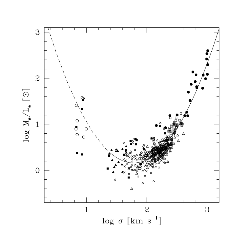
Figure 10.— An extended view of $M_{e}/L_{e}$ versus $\sigma$. To the data presented in Figure 9, we have added dEs and dSphs from Bender et al. (1992) (filled squares) and dSphs (open circles) from Mateo (1997). Five of the dSphs, at $\log\sigma\sim 1$, appear in both the Bender et al. (1992) and Mateo (1997) compilations, although the $M_{e}/L_{e}$ values are calculated in independent ways. For the Mateo (1997) data, we adopt the lower $M_{e}/L_{e}$ value if two are given. We also add a curve illustrating the best-fit parabola. We use a dashed line for $\log\sigma<1.4$ because the fit is unconstrained for these values. Neither the Bender et al. (1992) nor Mateo (1997) data are used in the fitting due to the large, possibly systematic, uncertainties. The simple parabola fits the data for systems ranging from dSphs to rich galaxy clusters.

We fit the data for dEs (Geha et al., 2003; Matkovic & Guzman, 2005), Es (Jørgensen et al, 1996), BCGs (Oegerle & Hoessel, 1991) and CSphs to a slightly rearranged version of Eq. 7, which we term the “fundamental manifold” in analogy to the FP,

$$\log r_{e}=-\alpha^{2}\log^{2}\sigma+(2+2\alpha\beta)\log\sigma+B\log I_{e}+C_{2}.$$

The resulting parameters are $\alpha^{2}=0.63\pm 0.02$, $(2+2\alpha\beta)=3.70\pm 0.07$, $B=-0.705\pm 0.004$ and $C^{\prime}=-2.75\pm 0.08$. If one uses only the ICS luminosity for the CSphs, then the resulting parameters are $\alpha^{2}=0.66\pm 0.02$, $(2+2\alpha\beta)=3.81\pm 0.08$, $B=-0.676\pm 0.004$ and $C^{\prime}=-2.90\pm 0.08$. The comparable plot to Figure 7 is shown in Figure 11 and the data used to obtain this fit are presented in Table 4. The rms scatter along the $r_{e}$ axis is now 0.099 for the combination of the Es, BCGs and CSphs (0.107 if the CSph is described by the ICS alone), which is not significantly worse than the 0.094 scatter of the elliptical FP alone. With the addition of the dwarf elliptical samples (Geha et al., 2003; Matkovic & Guzman, 2005)), the scatter rises to 0.114. The combined sample is highly weighted toward normal ellipticals, simply because they dominate the sample numerically, so it is important to examine the scatter carefully. For example, fitting a single FP to these same data results in a scatter of 0.129 between observed and fitted $r_{e}$, which is not much worse than that derived from the manifold fit. However, the rms deviation for the CSphs about the the manifold is 0.095, while it is 0.207 for the single FP fit. At the other extreme in the $\sigma$ range, the dEs from the Geha et al. (2003) sample have an rms deviation of 0.165 about the manifold and 0.256 about the single FP. The manifold results in significant improvements at both ends of the $\sigma$ range.

There are many reasons why our manifold fit must result in a scatter larger than the intrinsic scatter:

First, we combine data from various surveys carried out in different filters with different analysis techniques. Although we attempt to correct the colors to the same system, these corrections are based on mean observed or modeled colors for the population and mean filter+detector transmission curves.

Second, we do not correct for any wavelength dependence on $r_{e}$, which has been shown to exist at least for ellipticals (Pahre et al., 1998). While this is a systematic error within a given sample, in the merger of samples presented here it would increase the calculated scatter.

Third, we use the velocity dispersion of the cluster galaxies rather than the ICS. Theoretical modeling (Murante et al., 2004; Willman et al., 2004; Sommer-Larsen et al., 2005) and observations (Zibetti et al., 2005) conclude that the ICS is somewhat more centrally concentrated than the cluster galaxies, and hence could have somewhat different kinematics. Sommer-Larsen et al. (2005) suggest that at small radius the ICS could have about one-half the velocity dispersion of the galaxies. Indeed, a difference between the velocity dispersion of the cluster galaxies and ICS has been detected in the Coma cluster (Gerhard et al., 2005), although Kelson et al. (2002) find $\sigma_{ICS}\rightarrow\sigma$ at large radii in another cluster. If $\sigma$ is roughly a constant fraction or multiple of $\sigma_{ICS}$, then this difference would be absorbed into the constant term of Eq. 8. If $\sigma$ is only crudely related to $\sigma_{ICS}$, then we would find a large scatter in our relationships (making those relationships more difficult to identify). If the relationship between $\sigma$ and $\sigma_{ICS}$ depends on other cluster parameters, such as the concentration, then this would introduce a tilt in our relationships and move the CSphs away from the BCG FP. The continuity between the CSph and BCG FPs argues against this being a large effect. In any case, we expect any problems in using the galaxy velocity dispersion as a proxy for the ICS velocity dispersion to be an additional source of noise.

Figure 11.— Edge-on view of the 2-D manifold. Units given in text. All luminosities are corrected to the $I$-band (see text). Solid circles represent our CSph measurements, open squares the BCGs of Oegerle & Hoessel (1991), open triangles the Es of Jørgensen et al (1996), crosses the Es of Matkovic & Guzman (2005), and solid triangles the dEs of Geha et al. (2003). The line is the 1:1 line, and for this choice of axes it represents the best fit manifold.

Fourth, we apply no correction for non-sphericity, orbital anisotropy (cf. Ciotti et al., 1996), or rotation in any of these systems (cf. Busarello et al., 1997). While the rotation velocity of the ICS is presumably small in comparison to the velocity dispersion, the large ellipticity of the ICS components must at least necessitate a correction when converting from line-of-sight velocity dispersion to the velocity dispersion applicable for the FP.

Fifth, we do not correct the measured velocity dispersion to the velocity dispersion within $r_{e}$. As suggested by Sommer-Larsen et al. (2005), an additional complication is that this correction may be different for the galaxies than for the ICS.

Sixth, we ignore any direct dependence of $M_{e}/L_{e}$ on $I_{e}$ or $r_{e}$. To the degree that $\sigma$ can predict $I_{e}$ or $r_{e}$, we will model variations in $M_{e}/L_{e}$ with those parameters, but we know from the fact that spheroids do not fall on a fundamental line that $\sigma$ alone cannot reproduce the behavior in $I_{e}$ and $r_{e}$ exactly. In particular, we have not accounted for $B\neq 1$ in our scenario.

Seventh, we adopt the parabolic description of the relationship between $M_{e}/L_{e}$ and $\sigma$ as a mathematical convenience. The correct functional form could be asymmetric, or have a flatter bottom than a parabola, or less curvature. All of these issues suggest that the intrinsic scatter about the true “fundamental manifold” could be smaller than that measured here.

As with most explorations of the FP, one is left with intriguing relationships but no direct understanding of the physics that gives rise to those relationships. At the core of all of these fitting functions is the virial theorem, but it is the deviations from the simple expectations that can illuminate patterns in galaxy formation. In our case, we have two distinct results to understand: (1) why does $M_{e}/L_{e}$ rise with increasing $\sigma$ for large $\sigma$ and (2) why does $M_{e}/L_{e}$ rise with decreasing $\sigma$ for small $\sigma$? The balance between these two, possibly distinct, physical causes will account for the existence of the minimum $M_{e}/L_{e}$ and its particular value. In broad terms, and in different contexts, both of these trends have been noted before (generally for global $M/L$), and various investigators have attempted to explain them (cf. Babul & Rees, 1992; Martin, 1999; Benson et al., 2000; Marinoni & Hudson, 2002; van den Bosch et al., 2003; Dekel & Woo, 2003)). The behavior at low $\sigma$ has drawn more interest because 1) the observational effects — high $M_{e}/L_{e}$ (Mateo, 1997) and low effective yields (Garnett, 2002; Tremonti et al, 2004) — have been known for a longer time and 2) the formation history of low mass halos is critical in hierarchical models (Babul & Rees, 1992). Two primary processes are cited as responsible for the comparatively low star formation efficiency in low mass systems: winds and UV photoionization. One expects that supernova winds will more easily remove material in lower mass systems (Martin, 1999; Dekel & Woo, 2003) and that the intergalactic UV radiation field will more easily ionize the gas (Babul & Rees, 1992).

The behavior on the largest scales has been explored less, although Padmanabhan et al. (2004) found an analogous rise in $M/L$ as a function of mass among Es, and various groups have recently begun modeling the formation of the ICS (Murante et al., 2004; Willman et al., 2004; Sommer-Larsen et al., 2005). Those simulations predict that the ICS forms from the mergers of groups early in the history of the cluster. Because the ICS baryons are already in the form of stars at that stage, they behave much like the dark matter during the mergers. Therefore, they do not concentrate toward the center of the potential well and do not form systems with low $M_{e}/L_{e}$.

We conclude that the trend between $M_{e}/L_{e}$ and $\sigma$ describes how well baryons are able to dissipate and concentrate toward the center of the potential. The various driving factors are the degrees to which 1) the baryons have already been converted to stars prior to the assembly of the system, 2) new gas can cool and form stars in the final system, and 3) winds expel gas and lower the binding energy of the central component. Theoretical work is beginning to explore how mergers affect the relative distribution of dark and luminous matter (Boylan-Kolchin et al, 2005).

3.6. Interpreting the Minimum

The choice of a parabola to describe the $\log M_{e}/L_{e}$ versus $\log\sigma$ relation implies a well-defined global minimum in the relationship; however, we have stressed before that this particular functional form is somewhat arbitrary. Even so, the data, particularly for the dSphs, do suggest an upturn in $M_{e}/L_{e}$ at low $\sigma$, although a flat trough is not ruled out. If we accept the assumption of a parabolic relationship between $M_{e}/L_{e}$ and $\sigma$, our best fit manifold from Eq. 7 implies $\alpha=0.79\pm 0.03$ and $\beta=1.07\pm 0.05$ and that the minimum $M_{e}/L_{e}$ occurs in systems with $\sigma=22.9\pm 4.7$ km sec^-1. The degree to which these values are given physical significance is in large part determined by the validity of the mathematical form we have chosen, how well the various samples have been placed on the same photometric and kinematic systems, and the sampling of the data through the region of the minimum. Unfortunately, the bulk of our data are at larger $\sigma$ than the minimum and so our fit is quite sensitive to the limited data available near the minimum.

In contrast to what we did above, the turnover in the $M_{e}/L_{e}$ resulting from dimensional arguments (§3.4) occurs at $\sigma\sim 62$ km sec^-1 (Figure 10). While we have argued that the evaluation of $M_{e}/L_{e}$ using homology and dimensional arguments is not internally self-consistent with our modeling of the fundamental manifold (because of the higher order dependence of $\log M_{e}/L_{e}$ on $\log\sigma$ that we impose), these estimated values of $M_{e}/L_{e}$ do reflect something about the relationship between $\sigma$, $r_{e}$, and $I_{e}$. The reason the estimates do not agree in detail is presumably because the correct coefficients are not available in the dimensional argument and because the homology assumption breaks down. Which turnover is the more relevant in assessing the relative effects of winds, or photoionization, or structural changes due to the degree of dissipation is unclear. We conclude that while a change in behavior does occur, the exact value of $\sigma$ ranges between at least 20 to 60 km sec^-1. The corresponding mass scale is much lower than that suggested by studies of the global $M/L$ that also find a minimum $M/L$ at a specific mass scale (Benson et al., 2000; Marinoni & Hudson, 2002; van den Bosch et al., 2003), but the results are not necessarily in conflict. Observing differences in the behavior of $M/L$ within different radii, in this case within $r_{e}$ versus $r_{200}$, could potentially be used to break the degeneracy in the analysis between the dissipation of baryons and the efficiency of converting them to luminous matter.

3.7. Caveats

As with all analyses of the FP and its cousins, the description of spheroids as fully virialized, homologous (or at least weakly homologous) dynamical systems is oversimplistic. Our hope is that a minimalist description will embody the principal elements of spheroids, and the mere existence of the FP supports this approach. Nevertheless, to ignore the richness of the process of spheroid formation could lead to an overinterpretation of fortuitous coincidences. Even in the case of low scatter in the FP ($\sim$0.1), the scatter between observed and model $r_{e}$ is still 26%, which, while small considering the range of $r_{e}$ values, is not negligible. For the analysis and discussion we have presented, we remain concerned about the following:

We have ignored possible variations of $M_{e}/L_{e}$ that depend on $r_{e}$ and $I_{e}$. The standard approach attributes the tilt in the elliptical FP as being partly due to $\sigma$ and partly to the other terms in Eq. 4. We justify placing the entire burden on the form of the $\sigma$ term on the basis of the large variation in $A$ among FPs and the success of the model. However, given the various correlations between $r_{e}$, $I_{e}$, and $\sigma$ it is possible to slough off some of that variation to the other parameters. In a complete treatment, one would aim to explain the behavior of the $B$ coefficient in Eq. 8 as well as that of $A$. However, examining the residuals from the best fit manifold versus $I_{e}$, we find only a marginal indication of systematic behavior, and hence expect a minimal reduction in the scatter with the addition of a $I_{e}$-dependent term. Instead, we choose to limit the number of new parameters introduced at this stage, but, as samples increase, particularly for extremely low and high $\sigma$ spheroids, we anticipate more complex and complete modeling.

We have ignored other sources of homology breaking in our analysis. For example, systematic changes in orbital structure or in the dark matter potential as a function of spheroid scale will also tilt the FP. We argue that such changes cannot account for the large (factor of $\sim$ 100) difference in our calculated $M_{e}/L_{e}$ across the entire range of spheroids, but they are presumably there at some level. To the degree that they vary as a low-order function of $\sigma$, they are incorporated into Eq. 8.

We have focused on using the combination of BCG + ICS luminosity to describe the CSphs. In no other type of spheroid did we explicitly combine two components. Are CSphs truly described best by the combination, or are we being misled by small number statistics? Or do other systems, such as normal ellipticals, actually have a low surface brightness outer component, analogous to the ICS, that has not been observed? Regardless of whether we study the ICS alone, or in combination with the BCG, the existence of a fundamental manifold and the systematic behavior of $M_{e}/L_{e}$ with $\sigma$ remain (Figure 12).

The trends in $A$ and in $M_{e}/L_{e}$ are dominated by inter-sample differences rather than by intra-sample differences. Because the samples come from disparate analyses, we are concerned that some of the difference among them is due to systematic errors rather than physical causes. Because there is significant overlap between samples, we conclude that this is not a serious problem, but it is a fact that each of the principal samples alone is accurately described by a FP relation. Marginal evidence for curvature was noted by Jørgensen et al (1996) in their sample, although Bernardi et al. (2003) accounted for all the apparent curvature in their sample through selection effects.

Because most of the available data is on the high $\sigma$ side of the $M_{e}/L_{e}$ minimum, we have little constraint on the functional form of the $M_{e}/L_{e}-\sigma$ relation. For example, an equally reasonable attempt at unification could come by modeling the $M_{e}/L_{e}$ variation as a function of enclosed mass, $r_{e}\sigma^{2}$. This approach leads to an equation that is somewhat harder to interpret because of cross-terms, but that has the same number of free parameters. Even if the functional form, whatever it may be, is steeply rising on both sides (as reinforced by the dSph data), there is no reason to believe that the rise should be symmetric. Once one allows for asymmetry, the position of the minimum becomes quite uncertain and the need for data at $\log\sigma<1.5$ acute.

Figure 12.— Same as Figures 10 and 11 except the CSph luminosity is taken to be only that of the ICS, rather than that of the ICS+BCG. In the left panel, the solid line is the best fit parabola to the data shown in Figure 10 and is included here as a reference. In the right panel, $Y=3.81\log^{2}\sigma-0.66\log\sigma-0.68\log I_{e}-2.90$, and represents the best fit surface. Symbols are as described in Figure 10. Whether the CSph is described by the ICS or ICS+BCG does not affect either the relationship between $M_{e}/L_{e}$ and $\sigma$ or the nature of the fundamental manifold.

The interpretation of $r_{e}$ depends on the surface brightness profile. There is still some uncertainty in the literature regarding the relative merits of Sersíc versus deVaucouleur profiles across all spheroid classes. The latter type of profile is a special case of the former, so the more general statement that Sersić profiles fit spheroids is less controversial. A concern here is that there is a systematic trend in profile shape with $\sigma$ that produces corresponding systematic errors in $r_{e}$ and $I_{e}$, and hence in the FP. Bertin et al. (2002) have explored this topic and concluded that “weak” homology is satisfied, but the exact effect on an analysis such as ours is unclear. Graham & Guzmán (2003) find a continuous relationship in structural parameters of dEs to Es when they fit Sersíc profiles rather than $r^{1/4}$ profiles. Which profile is more appropriate across the full range of spheroids and how to compare among objects, different studies, and different methods are open questions. However, profile differences seem unlikely to result in the large FP differences observed among the full range of spheroids.

4. Conclusions

We demonstrate that spheroids ranging from dEs to the intracluster stellar component of galaxy clusters, which we designate the cluster spheroid (CSph), lie on a curved surface, a 2-D manifold, in $(\sigma,r_{e},I_{e})-$space. Previous studies have generally examined limited regions of parameter space, over which the manifold can be adequately described by a plane. Our principal findings are:

$\bullet$ The addition of cluster velocity dispersions, as measured from the cluster galaxies, decreases the scatter of the $r_{e}$-$I_{e}$ relation for the cluster spheroids, and therefore signifies the existence of a “fundamental plane” for clusters.

$\bullet$ Combining the luminosity of the brightest cluster galaxy (BCG) and the intracluster stars (ICS) leads to significantly lower scatter in the CSph FP relationship. We argue that this effect is real, implying a connection between the evolution of the BCG and ICS, rather than a poor decomposition of the two components. Our results do not change qualitatively if we use only the ICS for the CSph, but the scatter in various relationships increases significantly. Unless otherwise noted, we refer to the combination of BCG and ICS as the CSph, but in the more important cases present results for both descriptions of the CSph.

$\bullet$ The scatter of the CSph FP (0.074) is as small as that observed for elliptical galaxies, but the orientation of the plane is different.

$\bullet$ There is a systematic decline in the coefficient of the $\log\sigma$ term in the equation of the FP as one progresses from systems with smaller to larger $\sigma$. This trend suggests that a 2-D manifold, which over the limited range of $\sigma$ probed by any one spheroid population is indistinguishable from a plane, roughly forms a set of twisted planes that fit spheroids from low mass ellipticals to the CSphs of the most massive clusters.

$\bullet$ The non-linear relation between $\log M_{e}/L_{e}$ and $\sigma$ for spheroids implies a functional relation between these quantities that is more complex than a power law, and so requires the breaking of the homology assumption. We adopt $\log M_{e}/L_{e}=(\alpha\log\sigma-\beta)^{2}+\gamma$ as a model of this relationship because it reproduces the systematic decline in the coefficient of the $\log\sigma$ term in the FP equation and captures the curvature seen in the $\log M_{e}/L_{e}$ versus $\log\sigma$ relationship for spheroids. Of particular importance is that $M_{e}/L_{e}$ represents the mass to light ratio within $r_{e}$ and may be decoupled from the global $M/L$. The magnitude of the change in $M_{e}/L_{e}$ across the full range of spheroids excludes changes in stellar populations as a possible explanation for the global trend. Instead, these changes must be driven primarily by variations in the relative amounts of luminous and dark matter within $r_{e}$, although some modest dependence of $M_{e}/L_{e}$ with stellar populations must exist (see Cappellari et al. (2005) for a recent exploration of this topic for E’s).

$\bullet$ The resulting 2-D manifold has rms residuals along the $r_{e}$ axis of 0.099 (for Es, BCGs, and CSphs), compared to 0.094 for the FP plane fit to ellipticals alone and to 0.089 for BCGs alone. If we extend the manifold to dEs, the scatter increases slightly (0.114). The increased scatter relative to the individual FP’s of each spheroid population is insignificant given that the manifold fit is done with respect to five different samples that were observed in different photometric bands by different investigators. Using the best fit 2-D manifold to define the coefficients of the relationship between $\log M_{e}/L_{e}$ and $\log\sigma$, we find a minimum $M_{e}/L_{e}$ for galaxies with $\sigma=22.9\pm 4.7$ km s^-1. We qualitatively agree with a range of theoretical and observational studies that conclude that there exists a galaxy mass scale for which $M/L$ is minimized (Benson et al., 2000; Marinoni & Hudson, 2002; van den Bosch et al., 2003), although our value for that mass scale is significantly lower. Part of the discrepancy may arise from the measurement of this phenomenon on global scales, $r_{200}$, versus within $r_{e}$.

Our new description that places the family of spheroids on a 2-D manifold in $(\sigma,r_{e},I_{e})-$space is remarkable in that it unifies spheroids that span a factor of 100 in $\sigma$ and 1000 in $r_{e}$. This range of systems must have different histories both in terms of when they were assembled and when their stars formed. Even so, the global properties of these systems end up on the manifold with intrinsic scatter that must be less than 0.114 (30% in $r_{e}$). We are able to place all dark matter dominated spheroids on a single relation by accounting for the observed non-linear relationship between $\log(M_{e}/L_{e})$ and $\log\sigma$. This relationship, which deviates from simple virial theorem and homology expectations, points to a more specific phrasing of the question of how galaxies and clusters form: what is the origin of the relationship between $M_{e}/L_{e}$ and potential well depth? The relative importance of dissipation, cooling, star formation, feedback, and dynamical relaxation during spheroid formation must vary with spheroid scale in such a manner as to reproduce the continuous trend observed in $M_{e}/L_{e}$ (Figure 10), a trend responsible for the “fundamental manifold” (Figure 11). Theoretical explorations, such as those focusing on the interplay between different feedback mechanisms and the growth of galaxies (for examples, see Padmanabhan et al., 2004; Boylan-Kolchin et al, 2005; Dekel & Brinboim, 2005), may ultimately reveal the nature of the observed trend in $M_{e}/L_{e}$ and thereby unify the formation processes of spheroids.

References

- Babul & Rees (1992) Babul, A., & Rees, M.J. 1992, MNRAS, 255 346
- Bautz & Morgan (1970) Bautz, L. P. & Morgan, W. W. 1970, ApJ, 162, L149
- Beers et al. (1990) Beers, T.C., Flynn, K., & Gebhardt, K. 1990, AJ, 100, 32
- Bender et al. (1992) Bender, R., Burstein, D., & Faber, S.M. 1992, ApJ, 399, 462
- Bernardi et al. (2003) Bernardi, M. et al. 2003, AJ, 125, 1866
- Benson et al. (2000) Benson, A. J, Cole, S. Frenk, C. S. Baugh, C. M. & Lacey, C. G. 2000, MNRAS, 311, 793
- Bertin & Arnouts (1996) Bertin, E. & Arnouts, S. 1996, A&A, 117, 393
- Bertin et al. (2002) Bertin, G., Ciotti, L., & Del Principe, M 2002, A&A, 386, 149
- Boylan-Kolchin et al (2005) Boylan-Kolchin, M., Ma, C.-P., & Quateart, E. 2005, astro-ph/0502495
- Burke et al. (2000) Burke, D.J., Collins, C.A., & Mann, R.G. 2000, ApJ, 532, L105
- Burstein et al. (1997) Burstein, D., Bender, R., Faber, S., & Nolthenius, R. 1997, AJ, 114, 1365
- Busarello et al. (1997) Busarello, G., Capaccioli, M., Capozziello, S., Longo, G., & Puddu, E. 1997, A&A, 320, 415
- Cappellari et al. (2005) Cappellari, M. et al. 2005, MNRAS, in press (astro-ph/0505042)
- Carlberg (1986) Carlberg, R. G. 1986, ApJ, 310, 593
- Christlein & Zabludoff (2003) Chrsitlein, C. & Zabludoff, A.I. 2003, ApJ, 591, 764
- Ciotti et al. (1996) Ciotti, L., Lanzoni, B., & Renzini, A. 1996, MNRAS, 282, p 1
- Dekel & Brinboim (2005) Dekel, A., & Birnboim, Y. 2005, submitted (astro-ph/0412300)
- Dekel & Woo (2003) Dekel, A. & Woo, J. 2003, MNRAS, 344, 1131
- Dressler (1978) Dressler, A. 1978, ApJ, 223, 765
- Dressler et al. (1987) Dressler, A., Lynden-Bell, D., Burstein, D., Davies, R., Faber, S., Terlevich, R., & Wegner, G. 1987, ApJ, 313, 42
- Djorgovski & Davis (1987) Djorgovski, S., & Davis, M. 1987, ApJ, 313, 59
- Faber et al. (1987) Faber, S.M. et al. 1987, in Nearly Normal Galaxies: From the Planck Time to the Present, ed. S.M. Faber (NY: Springer), 175
- Feldmeier et al. (2002) Feldmeier, J. J., Mihos, J. C., Morrison, H. L., Rodney, S. A., & Harding, P. 2002, ApJ, 575, 779
- Feldmeier et al. (2004) Feldmeier, J. J., Mihos, C., Morrison, H. L., Harding, P., Kaib, N., & Dubinski, J. 2004, astro-ph/0403414
- Fukugita et al. (1995) Fukugita, M., Shimasaku, K., & Ichikawa, T. 1995, PASP, 107, 945
- Garnett (2002) Garnett, D.R. 2002, ApJ, 581, 1019
- Geha et al. (2003) Geha, M., Guhathakurta, P., van der Marel, R.P. 2000, ApJ, 126, 1794
- Gerhard et al. (2005) Gerhard, O., Arnaboldi, M., Freeman, K.C., Kashikawa, N., Okamura, S., and Yasuda, N. 2005, ApJ, 621, L93
- Gonzalez et al. (2000) Gonzalez, A. H., Zabludoff, A. I., Zaritsky, D., & Dalcanton, J. J. 2000, ApJ, 536, 561
- Gonzalez et al. (2005) Gonzalez, A.H., Zabludoff, A.I., & Zaritsky, D. 2005, ApJ, 618, 195 (Paper I)
- Graham & Guzmán (2003) Graham, A.W. & Guzmán, R. 2003, AJ, 125, 2936
- Hoessel et al. (1980) Hoessel, J.G., Gunn, J.E., & Thuan, T.X. 1980, ApJ, 241, 486
- Hudson & Ebeling (1997) Hudson, M.J. & Ebeling, H. 1997, ApJ, 479, 621
- Jørgensen et al (1996) Jørgensen, I., Franx, M., Kjaergaard, P. 1996, MNRAS, 280, 167
- Kelson et al. (2002) Kelson, D.D., Zabludoff, A.I., Williams, K.A., Trager, S.C., Mulchaey, J.S. & Bolte, M. 2002, ApJ, 576, 720
- Kormendy (1985) Kormendy, J. 1985, ApJ, 295, 73
- Lauer (1985) Lauer, T. R. 1985, ApJ, 292, 104
- Marinoni & Hudson (2002) Marinoni, C. & Hudson, M.J. 2002, ApJ, 569, 101
- Martin (1999) Martin, C.L. 1999, ApJ, 513, 156
- Mateo (1997) Mateo, M. 1997, ASPC 116 (Arnaboldi, M., Da Costa, G.S., and Saha, P. eds), 1997, pg. 259
- Matthews et al. (1964) Matthews, Morgan, & Schmidt 1964, ApJ, 140, 35
- Matkovic & Guzman (2005) Matkovic, A., & Guzman, R. 2005, MNRAS submitted
- Murante et al. (2004) Murante, G. et al. 2004, ApJ, 607, 83L
- Napolitano et al. (2005) Napolitano, N.R. et al. 2005, astro-ph/0411639
- Nelson et al. (2002) Nelson, A.E., Gonzalez, A.H., Zaritsky, D. & Dalcanton, J.J. 2002, ApJ, 566, 103
- Oegerle & Hoessel (1991) Oegerle, W.R. & Hoessel, J.G. 1991, ApJ, 375, 150
- Oemler (1973) Oemler, A. Jr. 1973, ApJ, 180, 11
- Oemler (1976) Oemler, A. Jr. 1976, ApJ, 209, 693
- Padmanabhan et al. (2004) Padmanabhan, N. et al. 2004, New Astronomy, 9, 329
- Pahre et al. (1998) Pahre, M.A., de Carvalho, R.R., & Djorgovski, S.G. 1998, AJ, 116, 1606
- Prugniel & Simien (1996) Prugniel, P., & Simien, F. 1996, A&A, 309, 749
- Schaeffer et al. (1993) Schaeffer, R., Mauforgordato, S., Cappi, A. & Bernardeau, F. 1993, MNRAS, 363, L21
- Scheick & Kuhn (1994) Scheick, X. & Kuhn, J. R. 1994, ApJ, 423, 566
- Schombert (1986) Schombert, J. M. 1986, ApJS, 60, 603
- Schombert (1987) Schombert, J. M. 1987, ApJS, 64, 643
- Schombert (1988) Schombert, J. M. 1988, ApJ, 328, 475
- Sommer-Larsen et al. (2005) Sommer-Larsen, J., Romeo, A.D., & Portinari, L. 2005, MNRAS, 357, 478
- Stiavelli et al. (2001) Stiavelli, M., Miller, B.W., Ferguson, H.C., Mack, J., Whitmore, B.C., & Lotz, J.M. 2001, AJ, 121, 1385
- Tremaine & Richstone (1977) Tremaine, S.D., & Richston, D.O. 1977, ApJ, 212, 311
- Tremonti et al (2004) Tremonti, C.A. et al. 2004, ApJ, 613, 898
- Trujillo et al. (2004) Trujillo, I, Burkert, A., & Bell, E.F. 2004, ApJ, 600, 39L
- Uson et al. (1990) Uson, J. M., Bough, S. P., & Kuhn, J. R. 1990, Science, 250, 539
- Uson et al. (1991) Uson, J. M., Bough, S. P., & Kuhn, J. R. 1991, ApJ, 369, 46
- van den Bosch et al. (2003) van den Bosch, F.C., Yang, X., & Mo, H.J. 2003, MNRAS, 340, 771
- Willman et al. (2004) Willman, B., Governato, F., Wadsley, J., & Quinn, T. 2004, MNRAS, 355, 159
- Yahil & Vidal (1977) Yahil, A., & Vidal, N. V. 1977, ApJ, 214, 347
- Zabludoff & Mulchaey (1998) Zabludoff, A.I., & Mulchaey, J.S. 1998, ApJ, 496, 39
- Zibetti et al. (2005) Zibetti, S., White, S.D.M., Schneider, D.P., & Brinkmann, J. 2005, MNRAS, 358, 949