High-resolution proper motions in a sunspot penumbra

Abstract

Local correlation tracking techniques are used to measure proper motions in a series of high angular resolution ($\sim$0$\farcs$1) penumbra images. If these motions trace true plasma motions, then we have detected converging flows that arrange the plasma in long narrow filaments co-spatial with dark penumbral filaments. Assuming that these flows are stationary, the vertical stratification of the atmosphere and the conservation of mass suggest downflows in the filaments of the order of 200 m s^-1. The association between downflows and dark features may be a sign of convection, as it happens with the non-magnetic granulation. Insufficient spatial resolution may explain why the estimated vertical velocities are not fast enough to supply the radiative losses of penumbrae.

1. Introduction

Sunspot penumbrae appear in the first telescopic observations of sunspots made four hundred years ago (see the historical introduction by Casanovas 1997). Despite this long observational record, we still lack of a physically consistent scenario to explain their structure, origin and nature. Penumbrae are probably a form of convection taking place in highly inclined strong magnetic fields (Danielson 1961; Thomas & Montesinos 1993; Schlichenmaier et al. 1998; Hurlburt et al. 2000; Weiss et al. 2004). However, there is no consensus even on this general description. For example, the observed vertical velocities do not suffice to transport the energy radiated away by penumbrae (e.g., Spruit 1987, and § 5), which has been used to argue that they are not exclusively a convective phenomenon. The difficulties of understanding and modeling penumbrae are almost certainly associated with the small length scale at which the relevant physical process take place. This limitation biases all observational descriptions, and it also makes the numerical modeling challenging and uncertain.

From an observational point of view, one approaches the problem of resolving the physically interesting scales by two means. First, assuming the existence of unresolved structure when analyzing the data, in particular, when interpreting the spectral line asymmetries (e.g., Bumba 1960; Grigorjev & Katz 1972; Golovko 1974; Sánchez Almeida & Lites 1992; Wiehr 1995; Solanki & Montavon 1993; Bellot Rubio 2004; Sánchez Almeida 2005a). Via line-fitting, and with a proper modeling, this indirect technique allows us to infer physical properties of unresolved structures. On the other hand, one gains spatial resolution by directly improving the image quality of the observations, which involves both the optical quality of the instrumentation and the application of image restoration techniques (e.g., Muller 1973a, b; Bonet et al. 1982, 2004, 2005; Stachnik et al. 1983; Lites et al. 1990; Title et al. 1993; Sütterlin et al. 2001; Scharmer et al. 2002; Rimmele 2004). Eventually, the two approaches have to be combined when the relevant length-scales are comparable to the photon mean-free-path (see, e.g., Sánchez Almeida 2001). The advent of the Swedish Solar Telescope (SST; Scharmer et al. 2003a, b) has opened up new possibilities along the second direct course. Equipped with adaptive optics (AO), it allows us to revisit old unsettled issues with unprecedented spatial resolution ($\sim$0$\farcs$1), a strategy which often brings up new observational results. In this sense the SST has already discovered a new penumbral structure, namely, dark lanes flanked by two bright filaments (Scharmer et al. 2002; Rouppe van der Voort et al. 2004). These dark cores in penumbral filaments were neither expected nor theoretically predicted, which reflects the gap between our understanding and the penumbral phenomenon.

The purpose of this work is to describe yet another new finding arising from SST observations of penumbrae. It turns out that the penumbral proper motions diverge away from bright filaments and converge toward dark penumbral filaments. We compute the proper motion velocity field employing the local correlation tracking method (LCT) described in the next section. Using the mean velocity field computed in this way, we follow the evolution of a set of tracers (corks) passively advected by the mean velocities. Independently of the details of this computation, the corks tend to form long narrow filaments that avoid the presence of bright filaments (Fig. 1b). This is the central finding of the paper, whose details uncertainties and consequences are discussed in the forthcoming sections. The behavior resembles the flows in the non-magnetic Sun associated with the granulation, mesogranulation, and supergranulation (e.g., November 1989; Title et al. 1989; Hirzberger et al. 1997; Wang et al. 1995a; Berger et al. 1998). The matter at the base of the photosphere moves horizontally from the sources of uprising plasma to the sinks in cold downflows. Using this resemblance to granular convection, we argue that the observed proper motions seem to indicate the existence of downward motions throughout penumbrae, and in doing so, they suggest the convective nature of the penumbral phenomenon.

LCT techniques have been applied to penumbrae observed with lower spatial resolution (see Wang & Zirin 1992; Denker 1998). Our analysis confirms previous findings of radial motions inward or outward depending on the distance to the penumbral border. In addition, we discover the convergence of these radial flows to form long coherent filaments.

The paper is organized as follows. The observations and data analysis are summarized in § 2. The proper motions of the small scale penumbral features are discussed in § 3 and § 4. The vertical velocities to be expected if the proper motions trace true mass motions are discussed in § 5, where we also consider their potential for convective transport in penumbrae. Finally, we elaborate on the implications of our finding in § 6. The (in-)dependence of the results on details of the algorithm is analyzed in Appendix A.

2. Observations and data analysis

We employ the original data set of Scharmer et al. (2002), generously offered for public use by the authors. They were obtained with the SST (Scharmer et al. 2003a, b), a refractor with a primary lens of 0.97 m and equipped with AO. The data were post-processed to render images near the diffraction limit. Specifically, we study the behavior of a penumbra in a 28 minutes long sequence with a cadence of 22 s between snapshots. The penumbra belongs to the large sunspot of the active region NOAA 10030, observed on July 15, 2002, close to the solar disk center (16° heliocentric angle). The series was processed with Joint Phase-Diverse Speckle (see Löfdahl & Scharmer 2003), which provides an angular resolution of 0$\farcs$12, close to the diffraction limit of the telescope at the working wavelength (G-band, $\lambda$ 4305 Å). The field-of-view (FOV) is $26\arcsec\,\times\,40\arcsec$, with pixels 0$\farcs$041 square. The images of the series were corrected for diurnal field rotation, rigid aligned, destretched, and subsonic Fourier filtered (modulations larger than 4 km s^-1 are suppressed). For additional details, see Scharmer et al. (2002) and the web page set up to distribute the data.

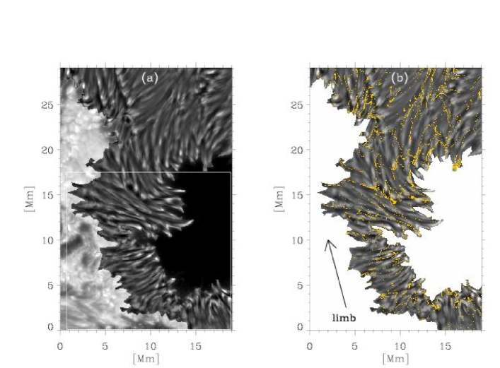
Figure 1.— (a) Mean image of the penumbra sharpened by removal of a spatial running mean of the original image. The figure also includes the umbra and sunspot surroundings for reference. (b) Image with the corks remaining in the penumbra after 110 min (the yellow dots). The corks form long narrow filaments that avoid the bright penumbral filaments (compare the two figures). The large arrow points out the direction of the closest solar limb.

Our work is devoted to the penumbra, a region which we select by visual inspection of the images. Figure 1a shows the full FOV with the penumbra artificially enhanced with respect of the umbra and the surrounding sunspot moat. Figure 1b shows the penumbra alone. The qualitative analysis carried out in the next sections refers to the lower half of the penumbra, enclosed by a white box in Fig. 1a. The results that we describe are more pronounced in here, perhaps, because the region is not under the influence of a neighbor penumbra outside but close to the upper part of our FOV. The effects of considering the full FOV are studied in Appendix A.

We compute proper motions using the local correlation tracking algorithm (LCT) of November & Simon (1988), as implemented by Molowny-Horas & Yi (1994). It works by selecting small sub-images around the same pixel in contiguous snapshots that are cross-correlated to find the displacement of best match. The procedure provides a displacement or proper motion per time step, which we average in time. These mean displacements give the (mean) proper motions analyzed in the work. The sub-images are defined using a 2D Gaussian window with smooth edges. The size of the window must be set according to the size of the structures selected as tracers. As a rule of thumb, the size of the window is half the size of the structure that is being tracked (see, e.g., Bonet et al. 2005). We adopt a window of FWHM 5 pixels ($\equiv$ 0$\farcs$2), tracking small features of about 10 pixels ($\equiv$ 0$\farcs$4). The LCT algorithm restricts the relative displacement between successive images to a maximum of 2 pixels. This limit constrains the reliability of the proper motion velocity components, $U_{x}$ and $U_{y}$, to a maximum of $\pm 2$ pix per time step, which corresponds to a maximum velocity of some 3.8 km s^-1. (Here and throughout the paper, the symbols $U_{x}$ and $U_{y}$ represent the two Cartesian components of the proper motions.) Such upper limit fits in well the threshold imposed on the original time series, were motions larger than 4 km s^-1  were filtered out by the subsonic filter.

Using the mean velocity field, we track the evolution of passively advected tracers (corks) spread out all over the penumbra at time equals zero. Thus we construct a cork movie (not to be confused with the 28 min long sequence of images from which the mean velocity field we inferred, which we call time series). The motions are integrated in time assuming 22 s per time step, i.e., the cadence of the time series. Figure 1b shows the corks that remain in the penumbra after 110 min. (The cork movie can be found in http://www.iac.es/proyect/solarhr/pencork.html.) Some 30 % of the original corks leave the penumbra toward the umbra, the photosphere around the sunspot, or the penumbra outside the FOV. The remaining 70 % are concentrated in long narrow filaments which occupy a small fraction of the penumbral area, since many corks end up in each single pixel. As it happens with the rest of the free parameters used to find the filaments, the final time is not critical and it was chosen by trial and error as a compromise that yields well defined cork filaments. Shorter times lead to fuzzier filaments, since the corks do not have enough time to concentrate. Longer times erase the filaments because the corks exit the penumbra or concentrate in a few sparse points.

We will compare the position of the cork filaments with the position of penumbral filaments in the intensity images. Identifying penumbral filaments is not free from ambiguity, though. What is regarded as a filament depends on the spatial resolution of the observation. (No matter whether the resolution is 2″  or 0$\farcs$1, penumbrae do show penumbral filaments. Obviously, the filaments appearing with 2″  and 0$\farcs$1 cannot correspond to the same structures.) Moreover, being dark or bright is a local concept. The bright filaments in a part of the penumbra can be darker than the dark filaments elsewhere (e.g., Grossmann-Doerth & Schmidt 1981). Keeping in mind these caveats, we use the average intensity along the observed time series to define bright and dark filaments, since it has the same spatial resolution as the LCT mean velocity map. In addition, the local mean intensity of this time average image is removed by subtraction of a running box mean of the average image. The removal of low spatial frequencies allows us to compare bright and dark filaments of different parts of the penumbra. The width of the box is set to 41 pixels or 1$\farcs$7. (This time averaged and sharpened intensity is the one represented in Figs. 1.)

The main trends and correlations to be described in the next sections are not very sensitive to the actual free parameters used to infer them (e.g., those defining the LCT and the local mean intensities). We have had to choose a particular set to provide quantitative estimates, but the variations resulting from using other sets are examined in Appendix A.

A final clarification may be needed. The physical properties of the corks forming the filaments will be characterized using histograms of physical quantities. We compare histograms at the beginning of the cork movie with histograms at the end. Except at time equals zero, several corks may coincide in a single pixel. In this case the corks are considered independently, so that each pixel contributes to a histogram as many times as the number of corks that it contains.

3. Proper motions

We employ the symbol ${\bf U}_{h}$ to denote the proper motion vector. Its magnitude $U_{h}$ is given by

$$U_{h}^{2}=U_{x}^{2}+U_{y}^{2},$$ (1)

with $U_{x}$ and $U_{y}$ the two Cartesian components. Note that these components are in a plane perpendicular to the line of sight. Since the sunspot is not at the disk center, this plane is not exactly parallel to the solar surface. However, the differences are insignificant for the kind of qualitative argumentation in the paper (see item # 7 in Appendix A). It is assumed that the plane of the proper motions defines the solar surface so that the $z$ direction corresponds to the solar radial direction. The solid line in Figure 2 shows the histogram of time-averaged horizontal velocities considering all the pixels in the penumbra selected for analysis (inside the box in Fig. 1a). The dotted line of the same figure corresponds to the distribution of velocities for the corks that form the filaments (Fig. 1b). The typical proper motions in the penumbra are of the order of half a km s^-1. Specifically, the mean and the standard deviation of the solid line in Fig. 2 are 0.51 km s^-1 and 0.42 km s^-1, respectively. With time, the corks originally spread all over the penumbra tend to move toward low horizontal velocities. The dotted line in Fig. 2 corresponds to the cork filaments in Fig. 1b, and it is characterized by a mean value of 0.21 km s^-1and a standard deviation of 0.35 km s^-1. This migration of the histogram toward low velocities is to be expected since the large proper motions expel the corks making it difficult to form filaments.

Figure 2.— Histogram of the horizontal velocities in the penumbra as inferred from LCT techniques. The solid line shows the whole set of penumbral points. The dotted line corresponds to the velocities at the positions of the corks after 110 min. The corks drift toward low horizontal velocity regions.

The proper motions are predominantly radial, i.e., parallel to the bright and dark penumbral filaments traced by the intensity. Figure 3 shows the distribution of angles between the horizontal gradient of intensity and the velocity. Using the symbol $I$ to represent the intensity image, the horizontal gradient of intensity $\nabla_{h}I$ is given in Cartesian coordinates by,

$$\nabla_{h}I=\Big{(}{{\partial I}\over{\partial x}}~{}~{}~{}~{}{{\partial I}\over{\partial y}}\Big{)}^{\dagger},$$ (2)

with the superscript ${\dagger}$ representing transpose matrix. The intensity gradients point out the direction perpendicular to the intensity filaments. The angle $\theta$ between the local velocity and the local gradient of intensity is

$$\cos\theta={{\nabla_{h}I}\over{|\nabla_{h}I|}}\cdot{{\bf U}_{h}\over{U_{h}}}.$$ (3)

The angles computed according to the previous expression tend to be around 90^∘ (Fig. 3), meaning that the velocities are perpendicular to the intensity gradients and so, parallel to the filaments.

Figure 3.— Histogram of the angle between the horizontal velocities and the horizontal gradients of intensity. They tend to be perpendicular (the histograms peak at $\theta\sim$ 90^∘). The same tendency characterizes both all penumbral points (the solid line), and those having cork filaments (the dotted line).

The radial motions tend to be inward in the inner penumbra and outward in the outer penumbra, a systematic behavior that can be inferred from Fig. 4. At the starting position of each cork (i.e., the position at time equals zero), Fig. 4 shows the intensity that the cork reaches by the end cork movie (i.e., at time equals 110 min). This forecast intensity image has a clear divide in the penumbra. Those points close enough to the photosphere around the sunspot will become bright, meaning that they exit the penumbra. The rest are dark implying that they either remain in the penumbra or move to the umbra.

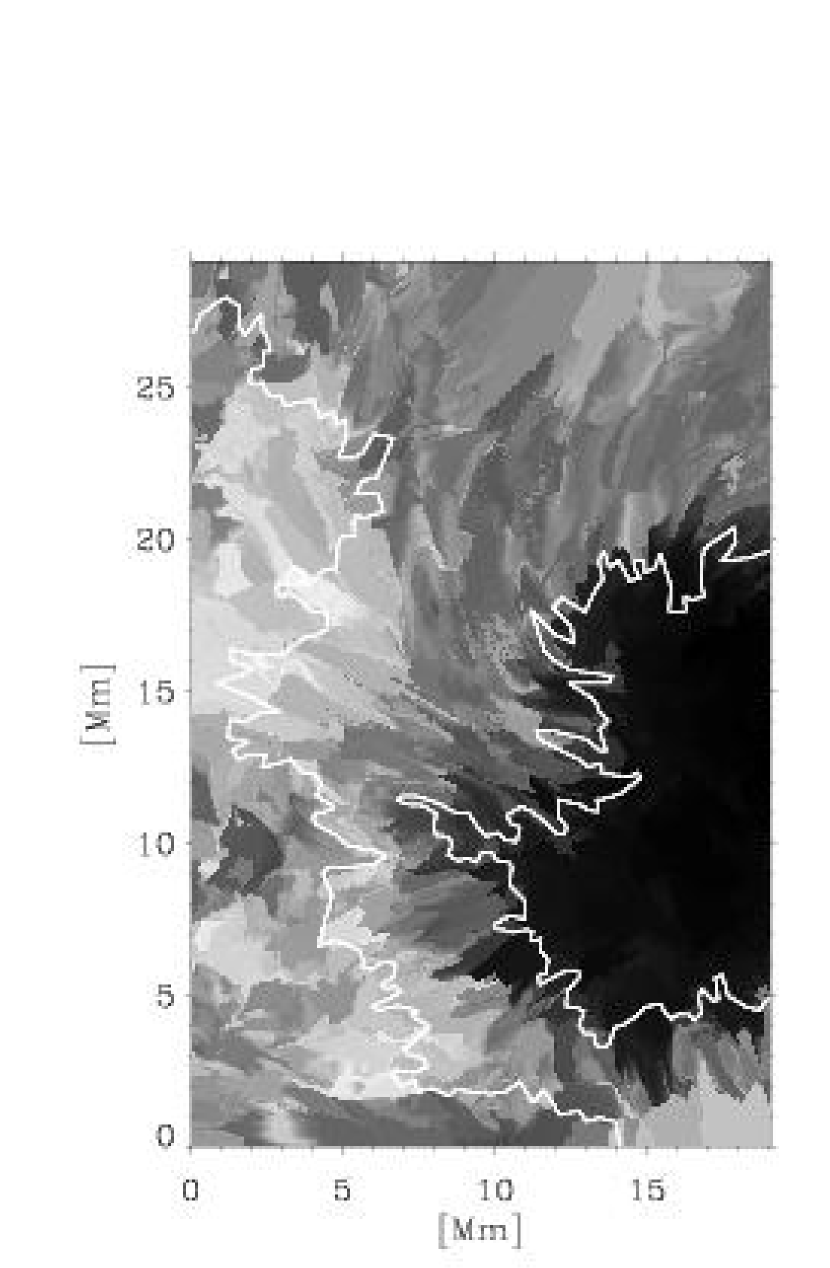
Figure 4.— Mapping of the final intensities that corks in each location of the FOV have by the end of the cork movie. The points in the outer penumbra tend to exit the sunspot, and so they are bright in this image. The points in the inner penumbra remain inside the sunspot, either within the penumbra or the umbra. The white contours outline the boundaries of the penumbra in Fig. 1. Points outside the penumbra are also included.

Such radial proper motions are well known in the penumbral literature (e.g., Muller 1973a; Denker 1998; Sobotka et al. 1999). However, on top of this predominantly radial flow, there is a small transverse velocity responsible for the accumulation of corks in filaments (§ 4).

The corks in Fig. 1b form long chains that avoid bright filaments and overlie dark filaments. The tracks followed by a set of corks finishing up in one of the filaments are plotted in Fig. 5.

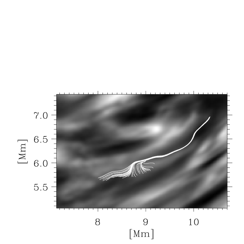
Figure 5.— Tracks followed by a set of 80 corks that end up in one of the cork filaments. The spatial coordinates have the same origin as those in Figs. 1 and 4.

It shows both the gathering at the head of the filament, and the tendency to avoid bright features where the narrow cork filament is formed. The migration of the corks toward dark penumbral filaments is quantified in Fig. 6a. It shows the histogram of intensities associated with the initially uniform distribution of corks throughout the penumbra (the solid line), and the final histogram after 110 min (the dotted line). A global shift toward dark locations is clear. The change is of the order of 20%, as defined by,

$$\Delta\mu/\sigma\equiv\big{[}\mu_{I}(110)-\mu_{I}(0)\big{]}/\sigma_{I}(0)\simeq-0.21,$$ (4)

with $\mu_{I}(t)$ the mean and $\sigma_{I}(t)$ the standard deviation of the histogram of intensities at time $t$ min. Figure 6b contains the same histogram as Fig. 6a but in a logarithm scale. It allows us to appreciate how the shift of the histogram is particularly enhanced in the tail of large intensities. The displacement between the two histograms is not larger because the corks do not end up in the darkest parts of the dark penumbral filaments (see, e.g., Fig. 5).

Figure 6.— (a) Histograms of the distribution of intensity associated with the cork filaments. The original distribution corresponds to corks uniformly spread out throughout the penumbra (the solid line). The dotted line represents the distribution at the cork filaments. Note the shift. All intensities are referred to the local mean intensity, which explains the existence of negative abscissae. (b) Same as (a) but in logarithm scale to appreciate the lack of very bright features associated with the cork filaments.

4. Formation of cork filaments

It is important to know which properties of the velocity field produce the formation of filaments. Most cork filaments are only a few pixels wide (say, from 1 to 3). The filaments are so narrow that they seem to trace particular stream lines, i.e., the 1D path followed by a test particle fed at the starting point of the filaments. Then the presence of a filament requires both a low value for the velocity in the filament, and a continuous source of corks at the starting point. The first property avoids the evacuation of the filament during the time span of the cork movie, and it is assessed by the results in § 3, Fig. 2. The second point allows the flow to collect the many corks that trace each filament (a single cork cannot outline a filament.) If the cork filaments are formed in this way, then their widths are independent of the LCT window width.

For the corks to gather, the stream lines of different corks have to converge. A convergent velocity field has the topology shown by the three solid line vectors in Fig. 7.

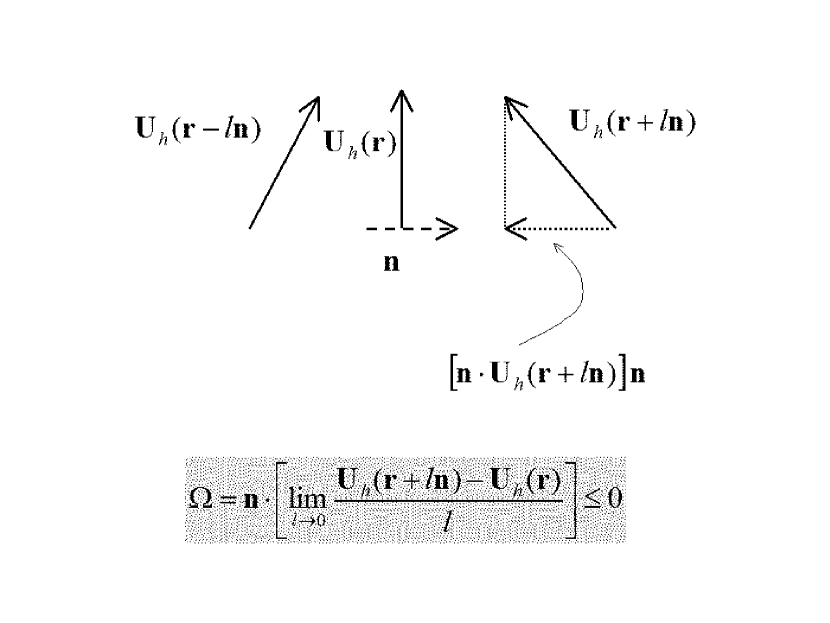
Figure 7.— The solid line vectors show three velocities of a convergent velocity field. The dashed line vector n corresponds to the vector normal to the velocity ${\bf U}_{h}$ in the point r, so that n$\cdot{\bf U}_{h}({\bf r})=0$. The dotted line vector shows the component of the velocity field parallel to n when moving along n. Note that it is anti-parallel to n, which implies that the directional gradient $\Omega$ is negative for convergent field lines.

As it is represented in the figure, the spatial variation of the velocity vector ${\bf U}_{h}$ in the direction n perpendicular to ${\bf U}_{h}$ is anti-parallel to ${\bf n}$. (${\bf U}_{h}\cdot{\bf n}=0$ with $|{\bf n}|=1$.) Consequently, the places where the velocities converge are those where $\Omega<0$, with

$$\Omega={\bf n}\cdot[({\bf n}\nabla_{h}){\bf U}_{h}].$$ (5)

The equation follows from the expression for the variation of a vector ${\bf U}_{h}$ in the direction of the vector n, which is given by $({\bf n}\nabla_{h}){\bf U}_{h}$ (e.g., Bronshtein & Semendyayev 1985, § 4.2.2.8). Then the component of this directional derivative in the direction normal to ${\bf U}_{h}$ is given by $\Omega$ in equation (5). The more negative $\Omega$ the larger the convergence rate of the velocity field. (Note that the arbitrary sign of n does not affect $\Omega$.) Using Cartesian coordinates in a plane, equation (5) turns out to be,

$$\Omega={{U_{x}^{2}}\over{U_{h}^{2}}}{{\partial U_{y}}\over{\partial y}}+{{U_{y}^{2}}\over{U_{h}^{2}}}{{\partial U_{x}}\over{\partial x}}-{{U_{x}U_{y}}\over{U_{h}^{2}}}\Big{[}{{\partial U_{y}}\over{\partial x}}+{{\partial U_{x}}\over{\partial y}}\Big{]}.$$ (6)

The histograms of $\Omega$ for all the pixels in the penumbra and for the cork filaments are shown in Fig. 8. Convergent and divergent flows coexist in the penumbra to give a mean $\Omega$ close to zero (the solid line is characterized by a mean of $4\times 10^{-5}$ s^-1 and a standard deviation of $1.8\times 10^{-3}$ s^-1). However, the cork filaments trace converging flows (the dotted line has a mean of $-1.1\times 10^{-3}$ s^-1 and a standard deviation of $2.7\times 10^{-3}$ s^-1). The typical $\Omega$ at the corks implies moderate convergent velocities, of the order of 100 m s^-1 for points separated by 100 km.

Figure 8.— Histograms of the derivative of the velocities in the direction perpendicular to the velocity field ($\Omega$; see its definition in the main text). As in previous figures, the solid line corresponds to all the pixels in the penumbra whereas the dotted line describes the cork filaments.

5. Discussion

Assume that the observed proper motions trace true mass motions. The horizontal velocities should be accompanied by vertical motions. In particular, those places traced by the cork filaments tend to collect mass that must be transported out of the observable layers by vertical motions. The need for mass conservation allows us to estimate the magnitude of such vertical velocities. Mass conservation in a stationary fluid implies that the divergence of the velocity field times the density is zero. This constraint leads to,

$$U_{z}\simeq h_{z}\Big{[}{{\partial U_{x}}\over{\partial x}}+{{\partial U_{y}}\over{\partial y}}\Big{]},$$ (7)

as proposed by November et al. (1987); November (1989). A detailed derivation of the equation is given in Appendix B. The symbol $h_{z}$ stands for the scale height of the flux of mass, which must be close to the density scale height (see November et al. 1987; November 1989). We want to stress that neither equation (7) assumes the plasma to be incompressible, nor $h_{z}$ is the scale height of $U_{z}$. Actually, the value of $h_{z}$, including its sign, is mostly set by the vertical stratification of density in the atmosphere (see Appendix B). Figure 9 shows histograms of $U_{z}$ computed using equation (7) with $h_{z}=100$ km. We adopt this scale height because it is close to, but smaller than, the figure measured in the non-magnetic Sun by November (1989, 150 km). The density scale hight decreases with temperature, which reduces the penumbral value with respect to that in the non-magnetic photosphere. (One can readily change to any other $h_{z}$ since it scales all vertical velocities.) According to Fig. 9, we find no preferred upflows or downflows in the penumbra. The solid line represents the histogram of $U_{z}$ considering all penumbral points; it has a mean of only $3\times 10^{-3}$ km s^-1 with a standard deviation of 0.39 km s^-1. However, the cork filaments prefer downflows. The dotted line shows the histogram of $U_{z}$ for the corks at the cork filaments. It has a mean of -0.20 km s^-1with a standard deviation of 0.36 km s^-1.

According to the arguments given above, the cork filaments seem to be associated with downflows. The cork filaments are also associated with dark features (§ 3). This combination characterizes the non-magnetic granulation (e.g. Spruit et al. 1990), and it reflects the presence of convective motions. The question arises as to whether the velocities that we infer can transport the radiative flux escaping from penumbrae. Back-of-the-envelope estimates yield the following relationship between convective energy flux $F_{c}$, mass density $\rho$, specific heat at constant pressure $c_{P}$, and temperature difference between upflows and downflows $\Delta T$,

$$F_{c}\simeq\rho|U_{z}|c_{P}\Delta T$$ (8)

(Spruit 1987). Following the arguments by Spruit (1987, § 3.5), the penumbral densities and temperature differences are similar to those observed in the quiet Sun. Furthermore $F_{c}$ is a large fraction of the quiet Sun flux (75 %). Then the vertical velocities required to account for the penumbral radiative losses are of the order of the velocities in the non-magnetic granulation or 1 km s^-1 (see also Schlichenmaier & Solanki 2003; Sánchez Almeida 2005b). One may argue that the penumbral vertical velocities inferred above are far too small to comply with such needs. However, the spatial resolution of our velocity maps is limited. The LCT detects the proper motions of structures twice the size of the window, or 0$\farcs$4 in our case (see § 2). The LCT smears the horizontal velocities and by doing so, it smears the vertical velocities too. Could this bias mask large vertical convective motions? We believe that it can, as inferred from the following argument. When the LCT procedure is applied to normal granulation, it leads to vertical velocities of a few hundred m s^-1, which are smaller than the fiducial figure required for equation (8) to account for the quiet Sun radiative flux (1 km s^-1). However, the quiet Sun radiative flux is deposited in the photosphere by convective motions. Therefore a large bias affects the quiet Sun estimates of vertical velocities based on LCT, and it is reasonable to conjecture that the same bias also affects our penumbral estimates. The vertical velocities associated with the non-magnetic solar granulation mentioned above have not been obtained from the literature. We have not been able to find any estimate when the LCT window has a size to track individual granules, say, 0$\farcs$7–0$\farcs$8. Then, we carried out an add hoc estimate using the quiet region outside the sunspot studied by Bonet et al. (2005). The vertical velocities are computed employing equation (7) when the FWHM of the LCT window equals 0$\farcs$75 . The inferred vertical velocities have standard deviations between 280 m s^-1 and 110 m s^-1 depending of the time average used to compute the mean velocities (5 min and 120 min, respectively). One can conclude that the vertical velocities are some five times smaller that the fiducial 1 km s^-1. This bias would increase our velocities to values consistent with the radiative losses of penumbrae.

Figure 9.— Histogram of the vertical velocities of the all the pixels in the penumbra (the solid line) and only those in the cork filaments (the dotted line). Upflows yield positive $U_{z}$. The corks seem to be preferentially associated with downflows of a few hundred m s^-1.

In short, given the limited spatial resolution, the velocities inferred from LCT may be underestimating the true vertical velocities. If this bias is similar to that affecting the non-magnetic granulation, then the observed velocities suffice to transport the radiative losses of penumbrae by convection.

All the discussion above assumes the proper motions to trace true motions. However, the proper motion velocities disagree with the plasma motions inferred from the Evershed effect, i.e., the intense and predominantly radial outward flows deduced from Doppler shifts (e.g., Solanki 2003; Thomas & Weiss 2004). Our proper motions are both inward and outward, and only of moderate speed (§ 3). This disagreement may cast doubts on the vertical velocities computed above. Fortunately, the doubts can be cleared up by acknowledging the existence of horizontal motions not revealed by the LCT technique, and then working out the consequences. Equation (7) is linear so that different velocity components contribute separately to $U_{z}$. In particular, the Evershed flow represents one more component, and it has to be added to the proper motion based vertical velocities. The properties of the Evershed flow at small spatial scales and large spatial scales do not modify the velocities in Figure (9). On the one hand, we apply equation (7) to average proper motions as inferred with the finite spatial resolution of our observations. It is a valid approach which, however, only provides average vertical velocities (see Appendix B). One has to consider the contribution of the average Evershed velocities, eliminating structures smaller than the spatial resolution of the proper motion measurements. On the other hand, the large scale structure of the Evershed flow is also inconsequential. According to equation (7), a fast but large spatial scale flow does not modify $U_{z}$; add a constant to $U_{x}$ and $U_{y}$, and $U_{z}$ does not change. Only the structure of the Evershed flow at intermediate spatial scales needs to be considered, and it does not invalidate our conclusion of downflows associated with the cork filaments. For the Evershed flow to invalidate this association, it would have to provide upflows co-spatial with the cork filaments, and so, with dark lanes. However, the existence of upflows in dark lanes is not favored by the observations of the Evershed effect, which seem to show the opposite, i.e., a local correlation between upflows and bright lanes (e.g., Beckers & Schröter 1969; Sánchez Almeida et al. 1993; Johannesson 1993; Schmidt & Schlichenmaier 2000). Thus we cannot rule out a bias of the vertical velocities in Figure (9) due to the Evershed flow but, if existing, the observed vertical component of the Evershed flow seems to reinforce rather than invalidate the relationship between cork filaments and downflows.

6. Conclusions

Using local correlation tracking (LCT) techniques, we measure mean proper motions in a series of high angular resolution (0$\farcs$12) penumbral images obtained with the 1-meter Swedish Solar Telescope (SST; Scharmer et al. 2002). Previous studies of lower resolution find predominantly radial proper motions, a result that we confirm. On top of this trend, however, we discover the convergence of the radial flows to form long coherent filaments. Motions diverge away from bright filaments to converge toward dark filaments. The behavior resembles the flows in the non-magnetic Sun associated with the granulation, where the matter moves horizontally from the sources of uprising plasma to the sinks in cold downflows. Using such similarity, we argue that the observed proper motions suggest the existence of downward flows throughout the penumbra, and so, they suggest the convective nature of the penumbral phenomenon. The places where the proper motions converge would mark sinks in the penumbral convective pattern.

The presence of this convergent motions is best evidenced using tracers passively advected as prescribed by the penumbral proper motion velocity field: see the dots in Fig. 1b and Fig. 5. With time, these tracers or corks form filaments that avoid the bright features and tend to coincide with dark structures. We quantify this tendency by following the time evolution of corks originally spread throughout the penumbra. After 110 min, the corks overlie features which are significantly fainter than the mean penumbra (the histogram of intensities is shifted by 20%; see § 3). Assuming that the proper motions reflect true stationary plasma motions, the need for mass conservation allows us to estimate the vertical velocities at the cork filaments, i.e., in those places where the plasma converges. These vertical velocities tend to be directed downward with a mean of the order of 200 m s^-1. The estimate is based on a number of hypotheses described in detail in §5 and Appendix B. We consider them to be reasonable but the fact that the vertical velocities are not direct measurements must be borne in mind. The inferred velocities are insufficient for the penumbral radiative flux to be transported by convective motions, which requires values of the order of 1 km s^-1. However, the finite spatial resolution leads to underestimating the true velocities, a bias whose existence is indicated by various results. In particular, the same estimate of vertical velocities applied to non-magnetic regions also leads to vertical velocities of a few hundred m s^-1, although we know from numerical simulations and observed Doppler shifts that the intrinsic granular velocities are much larger (e.g., Stein & Nordlund 1998; Beckers 1981).

The algorithm used to infer the presence and properties of the cork filaments depends on several free parameters, e.g., the size of the LCT window, the cadence, the time span of the cork movie, and so on. They were originally set by trial an error. In order to study the sensitivity of our results on them, the computation was repeated many times scanning the range of possible free parameters (Appendix A). This test shows how the presence of converging flows associated with dark lanes and downflows is a robust result, which does not depend on subtleties of the algorithms. It seems to depend on the spatial resolution of the observation, though.

The downward motions that we find may correspond to the ubiquitous downflows indirectly inferred by Sánchez Almeida (2005a) from the spectral line asymmetries observed in penumbrae. They may also be connected with an old observational result by Beckers & Schröter (1969), where they find a local correlation between brightness and Doppler shift with the same sign all over the penumbra, and so, corresponding to vertical velocities (see also, Sánchez Almeida et al. 1993; Johannesson 1993; Schmidt & Schlichenmaier 2000). The correlation is similar to that characterizing the non-magnetic granulation, which also suggests the presence of downflows in penumbrae. Analyses of spectroscopic and spectropolarimetric sunspot data indicate the presence of downflows in the external penumbral rim (e.g., Rimmele 1995; Schlichenmaier & Schmidt 2000; del Toro Iniesta et al. 2001; Bellot Rubio et al. 2003; Tritschler et al. 2004). The association between downflows and dark features is particularly clear in the 0$\farcs$2 angular resolution SST data studied by Langhans et al. (2005). Again, these downflows may be an spectroscopic counterpart of those that we infer. However, it should be clear that we also find downflows in the inner penumbra, where they do not. Whether this fact reflects a true inconsistency or can be easily remedied is not yet known.

Appendix A Robustness of the results

The various free parameters involved in the determination of proper motions were tunned by trial and error to favor the formation of narrow chains of corks in the dark penumbral lanes. However, the formation of such chains, their association with dark features, and the coincidence with locations of negative horizontal divergence are all robust results. We repeat the computation of proper motions and cork filament formation varying the free parameters. The results remain. This section gives a brief account of the study.

We start from the reference case, whose properties have been described in the main text (see also the first row in Table 1). Then each one of the parameters characterizing this reference case is varied maintaining the rest unchanged. The variation modifies velocities, intensities and angles, a change that we parameterize using the mean and standard deviation of the corresponding histograms. The actual tests are described below. Each one is associated with one or more rows in Table 1. The number in the first column of Table 1 facilitates the identification; it corresponds to the number in the list below. Such cross-reference is needed to follow some of the arguments.

Table 1Summary of uncertainties

	Case	$U_{h}$ [km s-1]		$\Delta\mu_{I}/\sigma_{I}$	$\theta~{}[^{\circ}]$		$U_{z}$ [km s-1]
		start	end		start	end	start	end
	reference	0.51$\pm$0.42	0.21$\pm$0.35	-0.21	91$\pm$40	89$\pm$42	0.00$\pm$0.39	-0.20$\pm$0.36
1	LCT 0$\farcs$12	0.57$\pm$0.48	0.23$\pm$0.41	-0.25	91$\pm$40	89$\pm$42	0.00$\pm$0.60	-0.44$\pm$0.66
1	LCT 0$\farcs$45	0.41$\pm$0.31	0.19$\pm$0.20	-0.18	91$\pm$42	91$\pm$45	0.01$\pm$0.17	-0.05$\pm$0.08
2	full penumbra	0.59$\pm$0.50	0.28$\pm$0.38	-0.16	90$\pm$41	91$\pm$43	0.00$\pm$0.42	-0.16$\pm$0.38
3	end time 37 min		0.26$\pm$0.30	-0.12		93$\pm$45		-0.14$\pm$0.32
3	end time 220 min		0.11$\pm$0.23	-0.28		83$\pm$40		-0.24$\pm$0.26
4	sharpened to 1$\farcs$3			-0.20	91$\pm$40	90$\pm$42
4	sharpened to 4$\farcs$1			-0.20	91$\pm$41	89$\pm$43
5	no velocity threshold	0.58$\pm$0.82	0.22$\pm$0.54	-0.19	91$\pm$40	89$\pm$42	0.00$\pm$0.83	-0.19$\pm$0.71
6	$D$ = 97 cm	0.48$\pm$0.38	0.16$\pm$0.23	-0.11	90$\pm$41	95$\pm$46	0.00$\pm$0.32	-0.21$\pm$0.24
6	$D$ = 80 cm	0.48$\pm$0.37	0.16$\pm$0.23	-0.08	90$\pm$41	92$\pm$46	0.00$\pm$0.31	-0.22$\pm$0.29
6	$D$ = 50 cm	0.47$\pm$0.35	0.15$\pm$0.19	-0.01	90$\pm$41	94$\pm$47	0.00$\pm$0.30	-0.24$\pm$0.25
7	Solar coordinates	0.52$\pm$0.49	0.26$\pm$0.48				0.01$\pm$0.40	-0.20$\pm$0.36
8	No destretching	0.55$\pm$0.43	0.20$\pm$0.32	-0.28	0.91$\pm$39	0.91$\pm$44	0.00$\pm$0.41	-0.28$\pm$0.44

1. We change the size of the LCT window to find out that the smaller the window the clearer the association of cork filaments with dark features and downflows. However, such association remains even for windows as large as 0$\farcs$45 FWHM.

2. The reference case analyzes the portion of penumbra within the box in Fig. 1a. When the whole FOV is used, then the cork filaments are not so dark and the mean downflows no so intense. However, all trends remain.

3. We choose the cork filaments as they appear after 110 min of evolution of the cork movie. This final time is not critical. The qualitative properties of the reference case are present right from the beginning of the movie, and they are enhanced as time increases. Table 1 includes means and standard deviations at two times, 37 min and 220 min. The latter has been computed assuming a time step of 44 s to integrate the cork movie. This fact also allows us to discard any significant effect of the time step on the results.

4. Changing the size of the box used to remove the local mean intensities changes the intensities used in our argumentation. However, the dependence is very moderate as attested by the figures in Table 1.

5. The LCT algorithm gives a few velocities larger than 2 pixels per time step (equivalent to 3.8 km s^-1), which is the largest displacement used to compute the cross-correlation function (§ 2). These large velocities result from a malfunction of the algorithm used to determine the optimum displacement. For this reason the reference case does not include velocities larger than 3.8 km s^-1. We checked that this threshold does not modify our results in significant way. We repeated the histograms for $U_{h}$, $\theta$, $I$ and $U_{z}$ including velocities larger than 3.8 km s^-1. The means of the histograms do not vary by more than 20 % (row number 5 in Table 1).

6. We investigate the role of the angular resolution of the images used to compute the proper motions and intensities. The 0$\farcs$12 angular resolution of the original time series was degraded as if it had been observed with an ideal telescope of diameter $D$. (Each snapshot of the series was convolved with the corresponding Airy disk.) The association between cork filaments and dark lanes shows up in the histograms only when the resolution of the degraded images is not far from the original one. It is almost gone when $D=50~{}$cm ($\Delta\mu_{I}/\sigma_{I}\sim-0.007$). Table 1 also includes the cases $D=80~{}$cm and $D=97~{}$cm. (Although the SST has $D=97~{}$cm, the original images were restored so that an ideal $D=97~{}$cm telescope does indeed reduce the contrast of the small structures used by the LCT algorithm to track.) It seems that the association between convergent proper motions and dark lanes depend critically on the angular resolution. This may explain why it has remained unnoticed in previous studies based on $D=50~{}$cm class telescopes.

7. We assume the horizontal and vertical velocities to be horizontal and vertical in a solar coordinate system. However the sunspot is slightly out of the disk center so that this assumption is only approximate. In order to evaluate the influence of this approximation, the three components of the velocity field were transformed to the true solar horizontal and vertical directions. (Two rotations are needed.) The transformation does not modify the histograms of velocities in a significant way; see Table 1.

8. The full analysis was repeated using the time series before destretching. The different snapshots were co-aligned assuming a rigid shift plus the rotation to be expected from the alt-azimuthal mounting of the SST. This new analysis does not differ in a significant way from reference case, so that the histograms seems to be independent of the application of a destretching algorithm to the data set.

Appendix B Derivation of equation (7)

This appendix provides a full derivation of equation (7) in the vein of the original derivation by November (1989). We contribute by considering the finite spatial resolution of the observations, and by discussing the validity of the approximation in the context of the magnetized penumbral plasma. Such a derivation was found to be necessary by various readers of the original manuscript, including the referees. The hypotheses are summarized in the final paragraph.

The continuity equation for a magnetized plasma with stationary flows is,

$$\nabla(\rho{\bf U})=0,$$ (B1)

with the symbols $\rho$ and U standing for the density and the velocity vector, respectively. The observations provide a kind of volume average of the velocities and densities, therefore, in order to apply equation (B1) to observables, the variables $\rho$ and ${\bf U}$ have to be replaced with volume averages. We model the volume averages as the convolution with a kernel describing the 3D region contributing to the observed signals. Using the property that partial derivatives and convolutions commute (e.g. Sánchez Almeida et al. 1996, § 2),

$$\langle\nabla(\rho{\bf U})\rangle=\nabla\langle\rho{\bf U}\rangle=0,$$ (B2)

where the angle brackets denote volume average. In general,

$$\langle\rho{\bf U}\rangle=\langle\rho\rangle\langle{\bf U}\rangle+\langle(\rho-\langle\rho\rangle)({\bf U}-\langle{\bf U}\rangle)\rangle.$$ (B3)

We will assume that the cross-correlation between the local fluctuations of density in the resolution element $\rho-\langle\rho\rangle$, and the fluctuations of velocity ${\bf U}-\langle{\bf U}\rangle$, are smaller than the product of the mean values, i.e.,

$$|\langle(\rho-\langle\rho\rangle)({\bf U}-\langle{\bf U}\rangle)\rangle|\ll|\langle\rho\rangle\langle{\bf U}\rangle|.$$ (B4)

Then,

$$\langle\rho{\bf U}\rangle\simeq\langle\rho\rangle\langle{\bf U}\rangle,$$ (B5)

and using equation (B2),

$$\nabla(\langle\rho\rangle\langle{\bf U}\rangle)\simeq 0.$$ (B6)

The inequality (B4) holds if the fluctuations of density are negligible, if the fluctuations of velocity are negligible, or if the fluctuations of density and velocity are uncorrelated. It is unclear whether any of these hypotheses alone justify the application of equation (B4) to penumbrae. However, the three of them can cooperate to make the cross correlation negligible, so it is not unreasonable to use equation (B4) as a working hypothesis, even for penumbrae.

The continuity equation for the actual variables (equation [B1]) and the mean variables (equation [B6]) are formally identical. We will use the former for the sake of clarity, dropping the angle brackets from the expressions (${\bf U}\equiv\langle{\bf U}\rangle$, and $\rho\equiv\langle\rho\rangle$). However, it must be clear that the densities and velocities appearing in all forthcoming equations correspond to the mean velocities and mean densities when the actual velocities and densities are averaged over a volume equivalent to the spatial resolution of the observations.

The density of the penumbral plasma presents two distinct types of variation. First, it varies depending on the magnetic field and temperature, with overdensities and underdensities that tend to cancel when computing the mean volume averaged density. This kind of variation is the only one existing in horizontal planes. Consequently, the horizontal variations of the mean density are much smaller than the true horizontal variations of density. Second, there is a systematic drop of density with the height in the atmosphere, as required for a plasma trying to be in equilibrium in a strong gravitational field. It is a systematic effect affecting all magnetic fields and temperatures and, therefore, it does not cancel in the mean density, which is expected to have a significant vertical variation. In mathematical parlance, the mean density at the spatial coordinates $x$, $y$ and $z$ can be split into two components,

$$\rho(x,y,z)=\rho_{0}(z)+\rho_{1}(x,y,z),$$ (B7)

with the one describing the systematic vertical variation $\rho_{0}$ larger than the other accounting for the horizontal variations $\rho_{1}$,

$$\rho_{1}\ll\rho_{0}.$$ (B8)

Keeping in mind this condition, the continuity equation can be approximated as,

$$\nabla\big{[}(\rho_{0}+\rho_{1}){\bf U}\big{]}\simeq\nabla(\rho_{0}{\bf U})=(\nabla\rho_{0})\cdot{\bf U}+\rho_{0}\nabla{\bf U}\simeq 0.$$ (B9)

Since $\rho_{0}$ only varies along the vertical direction then,

$$(\nabla\rho_{0})\cdot{\bf U}={{d\rho_{0}}\over{dz}}\,U_{z},$$ (B10)

and equation (B9) can be rewritten as,

$${{\partial U_{z}}\over{\partial z}}+{{d\ln\rho_{0}}\over{dz}}\,U_{z}+{{\partial U_{x}}\over{\partial x}}+{{\partial U_{y}}\over{\partial y}}\simeq 0,$$ (B11)

where the symbols $U_{x}$, $U_{y}$ and $U_{z}$ represent the three Cartesian components of the mean velocity field. With the density scale height $h_{\rho}$ defined as,

$$h_{\rho}^{-1}=-{{d\ln\rho_{0}}\over{dz}},$$ (B12)

and the vertical velocity scale height given by,

$$h_{u}^{-1}=-{{\partial\ln|U_{z}|}\over{\partial z}},$$ (B13)

equation (B11) can be expressed as,

$$U_{z}\simeq h_{z}\,\Big{[}{{\partial U_{x}}\over{\partial x}}+{{\partial U_{y}}\over{\partial y}}\Big{]},$$ (B14)

where the symbol $h_{z}$ represents the scale height of the vertical flux of mass,

$$h_{z}^{-1}=-{{\partial\ln|\rho_{0}U_{z}|}\over{\partial z}}=h_{\rho}^{-1}+h_{u}^{-1}.$$ (B15)

The expression (B14) corresponds to equation (7), which completes its derivation. Note that neither $h_{\rho}$ nor $h_{u}$ have been assumed to be constant, therefore, the densities and velocities do not necessarily have to vary exponentially.

An expression formally identical to equation (B14) is readily derived from equation (B1) under the unrealistic assumption of constant density. Then $\nabla{\bf U}=0$, which leads to equation (B14) with $h_{z}=h_{u}$. The inference of downflows associated with converging flows is based on the assumption $h_{z}>0$ (see § 5). In the unrealistic case of constant density, $h_{z}>0\Leftrightarrow h_{u}>0$, casting serious doubts on the inferred downflows since they follow fron the sign of $h_{u}$, which is unknown. However, the density is not constant and, consequently, one can have $h_{z}>0$ with vertical velocities whose magnitude $|U_{z}|$ decreases with height ($h_{u}>0$), increases with height ($h_{u}<0$), or is constant ($|h_{u}|\rightarrow\infty$). Although $h_{z}>0$ is an hypothesis, it seems to be more reasonable than the alternative $h_{z}<0$. The density is expected to decrease with height ($h_{\rho}>0$) and such a drop is inherited by the flux of mass, favoring $h_{z}>0$. In other words, for the assumption $h_{z}<0$ to hold one needs flows of unrealistic amplitude. Consider the following example. According to the arguments in the main text, $h_{\rho}\simeq 150$ km. Assume $h_{z}=-100$ km, so that the upflows and downflows are reversed with respect to those in Figure 9. Then equation (B15) renders $h_{u}=-60$ km, and so,

$$U_{z}(z)\simeq U_{z}(0)\,\exp(z/60\,{\rm km}).$$ (B16)

This law predicts large unobserved flows as soon as one moves up in the atmosphere. In the mid photosphere with $z=$150 km, an upflow of 0.5 km s^-1 at $z=0$ km is amplified to $U_{z}$(150 km)=6 km s^-1. Such extreme vertical velocities have not been observed questioning the underlying assumption $h_{z}<0$. Conversely, the positive $h_{z}$ used in the paper does not cause such problems; $h_{z}$=100 km with $h_{\rho}\simeq 150$ km lead to $h_{u}=300$ km and $U_{z}$(150 km)= 0.3 km s^-1.

To sum up, the hypotheses leading to equation (7) are: (a) the mean flows are stationary, (b) the cross-correlation between the fluctuations of density and velocity in the resolution element are smaller than the product of the mean values, and (c) the mean density varies mostly in the vertical direction.

References

- Beckers (1981) Beckers, J. M. 1981, in The Sun as a Star, ed. S. Jordan, NASA SP-450 (Washington: NASA), 11
- Beckers & Schröter (1969) Beckers, J. M., & Schröter, E. H. 1969, Sol. Phys., 10, 384
- Bellot Rubio (2004) Bellot Rubio, L. R. 2004, Rev. Mod. Astron., 17, 21
- Bellot Rubio et al. (2003) Bellot Rubio, L. R., Balthasar, H., Collados, M., & Schlichenmaier, R. 2003, A&A, 403, L47
- Berger et al. (1998) Berger, T. E., Löfdahl, M. G., Shine, R. A., & Title, A. M. 1998, ApJ, 506, 439
- Bonet et al. (2005) Bonet, J. A., Márquez, I., Muller, R., Sobotka, M., & Roudier, T. 2005, A&A, 430, 1089
- Bonet et al. (2004) Bonet, J. A., Márquez, I., Muller, R., Sobotka, M., & Tritschler, A. 2004, A&A, 423, 737
- Bonet et al. (1982) Bonet, J. A., Ponz, J. D., & Vazquez, M. 1982, Sol. Phys., 77, 69
- Bronshtein & Semendyayev (1985) Bronshtein, I. N., & Semendyayev, K. A. 1985, Handbook of Mathematics (New York: Van Nostrand Reinhold Company)
- Bumba (1960) Bumba, V. 1960, Izv. Crim. Astrophys. Obs., 23, 253
- Casanovas (1997) Casanovas, J. 1997, in ASP Conf. Ser., Vol. 118, Advances in the Physics of Sunspots, ed. B. Schmieder, J. C. del Toro Iniesta, & M. Vázquez (San Francisco: ASP), 3
- Danielson (1961) Danielson, R. E. 1961, ApJ, 134, 289
- del Toro Iniesta et al. (2001) del Toro Iniesta, J. C., Bellot Rubio, L. R., & Collados, M. 2001, ApJ, 549, L139
- Denker (1998) Denker, C. 1998, Sol. Phys., 180, 81
- Golovko (1974) Golovko, A. A. 1974, Sol. Phys., 37, 113
- Grigorjev & Katz (1972) Grigorjev, V. M., & Katz, J. M. 1972, Sol. Phys., 22, 119
- Grossmann-Doerth & Schmidt (1981) Grossmann-Doerth, U., & Schmidt, W. 1981, A&A, 95, 366
- Hirzberger et al. (1997) Hirzberger, J., Vazquez, M., Bonet, J. A., Hanslmeier, A., & Sobotka, M. 1997, ApJ, 480, 406
- Hurlburt et al. (2000) Hurlburt, N. E., Matthews, P. C., & Rucklidge, A. M. 2000, Sol. Phys., 192, 109
- Johannesson (1993) Johannesson, A. 1993, A&A, 273, 633
- Langhans et al. (2005) Langhans, K., Scharmer, G., Kiselman, D., Löfdahl, M., & Berger, T. E. 2005, A&A, 436, 1087
- Lites et al. (1990) Lites, B. W., Skumanich, A., & Scharmer, G. B. 1990, ApJ, 355, 329
- Löfdahl & Scharmer (2003) Löfdahl, M. G., & Scharmer, G. B. 2003, Proc. SPIE, 4853, 567
- Molowny-Horas & Yi (1994) Molowny-Horas, R., & Yi, Z. 1994, Internal Rep. 31,Institute of Theoretical Astrophysics, University of Oslo, Oslo
- Muller (1973a) Muller, R. 1973a, Sol. Phys., 29, 55
- Muller (1973b) —. 1973b, Sol. Phys., 32, 409
- November (1989) November, L. J. 1989, ApJ, 344, 494
- November & Simon (1988) November, L. J., & Simon, G. W. 1988, ApJ, 333, 427
- November et al. (1987) November, L. J., Simon, G. W., Tarbell, T. D., Title, A. M., & Ferguson, S. H. 1987, in NASA Conf. Pub., Vol. 2483, Theoretical Problems in High Resolution Solar Physics, ed. R. G. Athay & D. S. Spicer (Washington: NASA), 121
- Rimmele (1995) Rimmele, T. R. 1995, ApJ, 445, 511
- Rimmele (2004) —. 2004, ApJ, 604, 906
- Rouppe van der Voort et al. (2004) Rouppe van der Voort, L. H. M., Löfdahl, M. G., Kiselman, D., & Scharmer, G. B. 2004, A&A, 414, 717
- Sütterlin et al. (2001) Sütterlin, P., Rutten, R. J., & Skomorovsky, V. I. 2001, A&A, 378, 251
- Sánchez Almeida (2001) Sánchez Almeida, J. 2001, in ASP Conf. Ser., Vol. 248, Magnetic Fields Across the Hertzsprung-Russell Diagram, ed. G. Mathys, S. K. Solanki, & D. T. Wickramasinghe (San Francisco: ASP), 55
- Sánchez Almeida (2005a) Sánchez Almeida, J. 2005a, ApJ, 622, 1292
- Sánchez Almeida (2005b) —. 2005b, ApJ, in preparation
- Sánchez Almeida et al. (1996) Sánchez Almeida, J., Landi Degl’Innocenti, E., Martínez Pillet, V., & Lites, B. W. 1996, ApJ, 466, 537
- Sánchez Almeida & Lites (1992) Sánchez Almeida, J., & Lites, B. W. 1992, ApJ, 398, 359
- Sánchez Almeida et al. (1993) Sánchez Almeida, J., Martínez Pillet, V., Trujillo Bueno, J., & Lites, B. W. 1993, in ASP Conf. Ser., Vol. 46, The Magnetic and Velocity Fields of Solar Active Regions, ed. H. Zirin, G. Ai, & H. Wang (San Francisco: ASP), 192
- Scharmer et al. (2003a) Scharmer, G. B., Bjelksjö, K., Korhonen, T. K., Lindberg, B., & Petterson, B. 2003a, Proc. SPIE, 4853, 341
- Scharmer et al. (2003b) Scharmer, G. B., Dettori, P. M., Löfdahl, M. G., & Shand, M. 2003b, Proc. SPIE, 4853, 370
- Scharmer et al. (2002) Scharmer, G. B., Gudiksen, B. V., Kiselman, D., Löfdahl, M. G., & Rouppe van der Voort, L. H. M. 2002, Nature, 420, 151
- Schlichenmaier et al. (1998) Schlichenmaier, R., Jahn, K., & Schmidt, H. U. 1998, ApJ, 493, L121
- Schlichenmaier & Schmidt (2000) Schlichenmaier, R., & Schmidt, W. 2000, A&A, 358, 1122
- Schlichenmaier & Solanki (2003) Schlichenmaier, R., & Solanki, S. K. 2003, A&A, 411, 257
- Schmidt & Schlichenmaier (2000) Schmidt, W., & Schlichenmaier, R. 2000, A&A, 364, 829
- Sobotka et al. (1999) Sobotka, M., Brandt, P. N., & Simon, G. W. 1999, A&A, 348, 621
- Solanki (2003) Solanki, S. K. 2003, A&A Rev., 11, 153
- Solanki & Montavon (1993) Solanki, S. K., & Montavon, C. A. P. 1993, A&A, 275, 283
- Spruit (1987) Spruit, H. C. 1987, in The Role of Fine-Scale Magnetic Fields on the Structure of the Solar Atmosphere, ed. E.-H. Schrö ter, M. Váquez, & A. A. Wyller (Cambridge: Cambridge University Press), 199
- Spruit et al. (1990) Spruit, H. C., Nordlund, Å., & Title, A. M. 1990, ARA&A, 28, 263
- Stachnik et al. (1983) Stachnik, R. V., Nisenson, P., & Noyes, R. W. 1983, ApJ, 271, L37
- Stein & Nordlund (1998) Stein, R. F., & Nordlund, Å. 1998, ApJ, 499, 914
- Thomas & Montesinos (1993) Thomas, J. H., & Montesinos, B. 1993, ApJ, 407, 398
- Thomas & Weiss (2004) Thomas, J. H., & Weiss, N. O. 2004, ARA&A, 42, 517
- Title et al. (1993) Title, A. M., Frank, Z. A., Shine, R. A., Tarbell, T. D., Topka, K. P., Scharmer, G., & Schmidt, W. 1993, ApJ, 403, 780
- Title et al. (1989) Title, A. M., Tarbell, T. D., Topka, K. P., Ferguson, S. H., Shine, R. A., & SOUP Team. 1989, ApJ, 336, 475
- Tritschler et al. (2004) Tritschler, A., Schlichenmaier, R., Bellot Rubio, L. R., & the KAOS Team. 2004, A&A, 415, 717
- Wang & Zirin (1992) Wang, H., & Zirin, H. 1992, Sol. Phys., 140, 41
- Wang et al. (1995a) Wang, J., Wang, H., Tang, F., Lee, J. W., & Zirin, H. 1995a, Sol. Phys., 160, 277
- Wang et al. (1995b) Wang, Y., Noyes, R. W., Tarbell, T. D., & Title, A. M. 1995b, ApJ, 447, 419
- Weiss et al. (2004) Weiss, N. O., Thomas, J. H., Brummell, N. H., & Tobias, S. M. 2004, ApJ, 600, 1073
- Wiehr (1995) Wiehr, E. 1995, A&A, 298, L17