Comparison of dynamical model atmospheres of Mira variables with mid-infrared interferometric and spectroscopic observations

We present a comparison of dynamical model atmospheres with mid-infrared ($\sim$11 $\mu$m) interferometric and spectroscopic observations of the Mira variable $o$ Cet. The dynamical model atmospheres of Mira variables pulsating in the fundamental mode can fairly explain, without assuming ad-hoc components, the seemingly contradictory mid-infrared spectroscopic and interferometric observations of $o$ Cet: the 11 $\mu$m sizes measured in the bandpass without any salient spectral features are about twice as large as those measured in the near-infrared. Our calculations of synthetic spectra show that the strong absorption due to a number of optically thick H₂O lines is filled in by the emission of these H₂O lines originating in the geometrically extended layers, providing a possible physical explanation for the picture proposed by Ohnaka (2004a ) based on a semi-empirical modeling. This filling-in effect results in rather featureless, continuum-like spectra in rough agreement with the observed high-resolution 11 $\mu$m spectra, although the models still predict the H₂O lines to be more pronounced than the observations. The inverse P-Cyg profiles of some strong H₂O lines observed in the 11 $\mu$m spectra can also be reasonably reproduced by our dynamical model atmospheres. The presence of the extended H₂O layers manifests itself as mid-infrared angular diameters much larger than the continuum diameter. The 11 $\mu$m uniform-disk diameters predicted by our dynamical model atmospheres are in fair agreement with those observed with the Infrared Spatial Interferometer (ISI), but still somewhat smaller than the observed diameters. We discuss possible reasons for this discrepancy and problems with the current dynamical model atmospheres of Mira variables.

1 Introduction

Mira variables exhibit large-amplitude pulsation, which leads to remarkable temporal variations of brightness, effective temperature, and geometrical extension of the atmosphere. A better understanding of the structure of such dynamical atmospheres is crucial for unraveling the mass loss mechanism in these stars. Recent interferometric observations in the near-infrared as well as in the mid-infrared have revealed that the angular diameters of Mira variables increase toward longer wavelengths. Mennesson et al. (mennesson02 (2002)) show that the $L^{\prime}$-band diameters of Mira variables are 20–100% larger than those measured in the $K^{\prime}$ band. Millan-Gabet et al. (millan-gabet05 (2005)) carried out angular diameter measurements in the $J$, $H$, and $K$ bands for a number of Mira variables and show the general trend: $J$-band diameter $<$ $H$-band diameter $<$ $K$-band diameter. This trend extends into the mid-infrared, as demonstrated by the 11 $\mu$m observations of Weiner et al. (weiner00 (2000), 2003a , and 2003b , hereafter W00, WHT03a, WHT03b, respectively) using ISI. They found that the 11 $\mu$m diameters of the Mira variables $o$ Cet, R Leo, and $\chi$ Cyg are approximately twice as large as those observed in the $K$ band. In the optical, on the other hand, the angular sizes of Mira variables increase systematically toward shorter wavelengths, from 1 $\mu$m down to 0.65 $\mu$m, as Ireland et al. (2004a ) have recently shown.

Such wavelength dependence of the angular sizes of Mira variables has often been attributed to dust shells, whose flux contribution due to dust thermal emission increases from the near-infrared to the mid-infrared. In fact, the inner region of dust shells around Mira variables has been studied using mid-infrared interferometric data (e.g., Danchi et al. danchi94 (1994); Tevousjan et al. tevousjan04 (2004); Ohnaka et al. ohnaka05 (2005)). The increase of the angular sizes toward shorter wavelengths in the optical can also be attributed to the increase of scattered light due to dust grains (e.g., Ireland et al. 2004a ). Optical interferometric polarimetry of Mira variables carried out by Ireland et al. (ireland05 (2005)) also suggests that the scattering due to dust grains is responsible for the systematic increase of the angular size shortward of $\sim$1 $\mu$m.

Nevertheless, the increase of the angular sizes of Mira variables from the near-infrared to the mid-infrared revealed by the 11 $\mu$m ISI observations of W00, WHT03a, and WHT03b cannot be solely attributed to the presence of extended dust shells for the following reason. The presence of an extended dust shell well separated from the underlying atmosphere leads to a steep drop of visibilities that appears only at low spatial frequencies, and the effect of such an extended dust shell is to lower the total visibility by an amount equal to the fractional flux contribution of the dust shell at the wavelength at issue. This effect is already taken into account in the derivation of the 11 $\mu$m uniform-disk diameters by W00, WHT03a, and WHT03b. Still, the angular sizes obtained at 11 $\mu$m are by a factor of $\sim$2 larger than those measured in the near-infrared.

On the other hand, there is mounting evidence suggesting that gaseous layers extending to a few stellar radii are responsible for the increase of the angular size from the near-infrared to the mid-infrared. Mennesson et al. (mennesson02 (2002)) as well as Schuller et al. (schuller04 (2004)) suggested that the increase of the angular sizes of Mira variables from the $K$ band to the $L^{\prime}$ band may be attributed to extended gaseous layers. Perrin et al. (perrin04 (2004)) attempted to interpret the visibilities of Mira variables observed in the near-infrared as well as in the 11 $\mu$m region, using a model of a molecular shell where the molecular opacity and its wavelength dependence were treated as free parameters rather than calculated from detailed line lists. They conclude that the observed near-infrared and 11 $\mu$m visibilities can be reproduced by shells extending to $\sim$2.2 $R_{\star}$ with temperatures of 1500–2000 K and optical depths of 0.2–1.2 at 2.03 $\mu$m. Weiner (weiner04 (2004)) used a similar model but with molecular opacities calculated from the detailed H₂O line list of Partridge & Schwenke (partridge97 (1997), hereafter PS97) and reached a similar conclusion based on the model fitting to the near-infrared and 11 $\mu$m visibilities of $o$ Cet.

Then, the high-resolution 11 $\mu$m spectra of Mira variables presented by WHT03a and WHT03b have appeared as a puzzling piece to this picture. These spectra obtained using the TEXES instrument with a spectral resolution of $\sim\!\!\!10^{5}$ (Lacy et al. lacy02 (2002)) show that no salient spectral feature is present within the narrow bandpasses used in the ISI observations, and this absence of spectral features appears to contradict the interpretation that the molecular layers close to the star are responsible for the increase of the angular size from the near-infrared to the mid-infrared. While the 11 $\mu$m spectra were not calculated or not well reproduced by Perrin et al. (perrin04 (2004)) or Weiner (weiner04 (2004)), Ohnaka (2004a ) demonstrates that the angular diameters and high-resolution spectra of Mira variables obtained in the 11 $\mu$m region can be simultaneously explained by an optically thick, dense warm water vapor envelope. Using a two-layer model for this warm water vapor envelope, Ohnaka (2004a ) found that the absorption due to the dense water vapor is filled in by emission from the extended part of the water vapor envelope, making the spectra almost featureless. On the other hand, the presence of the water vapor envelope manifests itself as an increase of the angular diameter from the near-infrared to the mid-infrared.

While such ad-hoc models do not address the question about the physical processes responsible for the formation of the warm water vapor envelope, they are useful for illustrating the basic picture of the outer atmosphere and deriving its approximate physical properties, providing us with insights on possible next steps. In fact, Ohnaka (2004a ) shows that the intensity profiles predicted by the two-layer model for the warm water vapor envelope resemble those predicted by the dynamical models studied by Tej et al. (2003a ), suggesting the possibility that the large-amplitude pulsation in Mira variables may be responsible for the existence of the warm water vapor envelope.

In the present paper, we examine this possibility by comparing the observed 11 $\mu$m diameter and the high-resolution spectra of $o$ Cet with those predicted by dynamical model atmospheres.

2 Dynamical model atmospheres

Table 1: Summary of dynamical models used in the present work. $R_{1.04}$ is the radius defined by the position of the layer where the optical depth in the 1.04 $\mu$m continuum is equal to unity. $R_{\rm p}$ is the Rosseland radius of the parent star, which is an initial, static model. The P models have $R_{\rm p}$ = 241 $R_{\sun}$, while the M models have $R_{\rm p}$ = 260 $R_{\sun}$. $T_{\rm eff}$ is defined as $(L/4\pi\sigma R_{\rm Ross}^{2})^{1/4}$, where $R_{\rm Ross}$ is the Rosseland radius of a dynamical model, and $\sigma$ is the Stefan-Boltzmann constant. $T_{\rm 1.04}=(L/4\pi\sigma R_{1.04}^{2})^{1/4}$ gives a representative temperature of the continuum-forming layers.

Model	Cycle+Phase	$R_{1.04}$/$R_{\rm p}$	$T_{\rm eff}$ (K)	$T_{\rm 1.04}$ (K)	$L$ ($L_{\sun}$)
P05	0+0.5	0.90	2160	2500	1650
P12	1+0.23	1.30	2610	2680	4540
P13n	1+0.30	1.26	2310	2530	3450
P14n	1+0.40	1.19	2080	2510	2920
P15n	1+0.50	0.84	1800	2690	1910
P22	2+0.18	1.26	2640	2700	4400
P23n	2+0.30	1.24	2470	2590	3570
P24n	2+0.40	1.16	2210	2420	2380
P25	2+0.53	0.91	2200	2500	1680
P35	3+0.5	0.81	2270	2680	1760
M05	0+0.49	0.84	2310	2420	1470
M12n	1+0.21	1.18	2410	2540	3470
M14n	1+0.40	0.91	2110	2400	1670
M15	1+0.48	0.83	2460	2530	1720
M22	2+0.25	1.10	2330	2490	2850
M23n	2+0.30	1.03	2230	2460	2350
M24n	2+0.40	0.87	2160	2410	1540
M25n	2+0.50	0.79	2770	2780	2250

Since the details of the dynamical model atmospheres used in the present work are described in Hofmann et al. (hofmann98 (1998)), Tej et al. (2003b ), Ireland et al. (2004b ), and Ireland et al. (2004c ) (hereafter, HSW98, TLSW03, ISW04, and ISTW04, respectively), we only summarize the properties of the models, in particular those relevant to our calculations. These dynamical model atmospheres are specified by the period, stellar mass, luminosity, and Rosseland radius of the static parent star, which is an initial model before the star is brought into self-excited pulsation. In the present work, we use the P and M series, as given in Table LABEL:table_model. Both P and M models are fundamental-mode pulsators with a period of 332 days, a parent-star luminosity of 3470 $L_{\sun}$, and masses of 1.0 $M_{\sun}$ (P series) and 1.2 $M_{\sun}$ (M series). Here, 332 days is the formal period of the parent star, whereas the actual periods of the dynamical models are slightly different (P models: 341 days; M models: 317 days; $o$ Cet: 334 days; see ISTW04). Throughout the present work, we define the continuum radius by the position of the layer where the optical depth measured in the continuum at 1.04 $\mu$m is equal to unity. The Rosseland radius, which is also used as a “stellar radius” in some works, is often close to the 1.04 $\mu$m continuum radius. It should be mentioned, however, that it is not always the case, as discussed in ISW04 and ISTW04.

Comparison of dynamical model atmospheres with various observations implies that Mira variables are fundamental-mode pulsators. Woodruff et al. (woodruff04 (2004)) have recently analyzed the $K$-band interferometric data on $o$ Cet obtained with VLTI/VINCI and compared the visibilities observed at phases from $\sim$0.1 to $\sim$0.5 with those predicted by dynamical model atmospheres in the fundamental mode (including the P and M models) as well as in the first overtone mode. They show that the observed visibilities can be best explained by the dynamical models pulsating in the fundamental mode. The Rosseland radius derived from the observed visibilities is found to be consistent with the period-radius-relation of the fundamental-pulsator models, but not with that of the models pulsating in the first overtone mode. The analysis of Woodruff et al. (woodruff04 (2004)) further suggests the P model as the best-fit model for the VINCI observations of $o$ Cet. Fedele et al. (fedele05 (2005)) have also obtained a similar result for another Mira variable, R Leo, based on the analysis of the VINCI data. These results on the pulsation mode of Mira variables are consistent with the conclusion drawn by Wood et al. (wood99 (1999)) from the comparison of theoretical pulsation models with MACHO observations of long period variables in the Large Magellanic Cloud as well as with the pulsation velocities derived from line profiles (Scholz & Wood scholz00 (2000)).

Using the density stratification obtained by a self-excited pulsation model at a given cycle and phase, the temperature stratification and molecular/atomic abundances in the non-gray atmosphere are calculated with the assumption of local thermodynamical equilibrium (LTE) and radiative equilibrium in spherical symmetry, as described in Bessell et al. (bessell96 (1996)) and HSW98. The solar chemical composition is used in the calculations of these atmospheric models. The next step is to calculate intensity profiles as well as synthetic spectra in the 11 $\mu$m region using the temperature and density stratifications and the velocity field of each model. For the positions and the transition probabilities of H₂O lines, we use the HITEMP database (Rothman rothman97 (1997)) as well as the line list compiled by PS97, which is deemed to be the most extensive line list of H₂O to date. The line shape in the rest frame is assumed to be a Voigt profile with a micro-turbulent velocity of 5 km s^-1, which is close to the value derived for the Mira variable R Leo by Hinkle & Barnes (hinkle79 (1979)). The monochromatic intensity profile is calculated by evaluating the intensity at multiple impact parameters with respect to the stellar disk in the observer’s frame (e.g., Mihalas mihalas78 (1978)), with the radial velocity of each layer taken into account. The monochromatic visibility can be obtained by taking the Hankel transform (two-dimensional Fourier transform in a centrosymmetric case) of the monochromatic intensity profile. In the calculation of visibilities, we adopt a distance of 107 pc to $o$ Cet based on the HIPPARCOS parallax (Knapp et al. knapp03 (2003); see also the discussion of ISTW04 about the distance of $o$ Cet).

The monochromatic intensity profiles as well as the monochromatic visibilities calculated in the relevant wavelength region are then spectrally convolved with a response function, which represents the bandpass used in the ISI observations. As described in Ohnaka (2004a , 2004b ), we approximate the response function with a top-hat function with a width of 0.17 cm^-1. When comparing model visibilities calculated in this manner with those observed, it is necessary to take the flux contribution of an extended dust shell into account. The presence of such a dust shell appears as a steep visibility drop at low spatial frequencies and lowers the visibility resulting from the underlying atmosphere by an amount equal to the fractional flux contribution of the dust shell. Therefore, the total visibility $V_{\omega}^{\rm total}$, which can be compared with the ISI observations, is calculated as

$$V_{\omega}^{\rm total}=(1-f_{\rm dust})V_{\omega}^{\rm atm}\,,$$ (1)

where $f_{\rm dust}$ is a constant representing the fraction of the continuous dust emission from the dust shell in the 11 $\mu$m region, and $V_{\omega}^{\rm atm}$ is the (spectrally convolved) visibility predicted by the atmospheric models. The spectrum (i.e., emergent flux) is obtained by integrating the intensity over the stellar disk. The spectrum is then convolved with a Gaussian representing the resolution of the spectroscopic instrument and the macro-turbulent velocity in the atmosphere of Miras. The spectral resolution of the TEXES instrument corresponds to $\sim$3 km s^-1, and we adopt a macro-turbulent velocity of 3 km s^-1, as assumed in Ohnaka (2004a ). This leads to a Gaussian with a FWHM of 4.24 km s^-1. In order to take into account the flux contribution of the dust shell, which amounts up to $\sim$60–70% in the mid-infrared, the convolved and normalized spectrum is diluted as follows:

$$F_{\omega}^{\rm diluted}=(1-f_{\rm dust})F_{\omega}+f_{\rm dust}\,,$$ (2)

where $F_{\omega}^{\rm diluted}$ is the final spectrum, and $F_{\omega}$ is the spectrum emerging from the atmosphere without the presence of a dust shell.

3 Comparison with the observed spectra and angular diameters

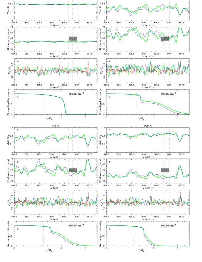
Figure 1: Comparison of the mid-infrared interferometric and spectroscopic observations with the predictions of selected P models. At each phase, the panels a, b, c, and d show the predicted visibilities, uniform-disk diameters, spectra, and intensity profiles at 896.85 cm^-1, respectively. In all panels, the model predictions using the HITEMP database and the PS97 line list are represented with the thick (green) and thin (blue) solid lines, respectively. The visibilities and uniform-disk diameters are derived for a projected baseline length of 30 m. In the panel b, the dashed lines represent the bandpasses used in the ISI observations, and the range of the uniform-disk diameters observed with ISI at relevant phases, from 0.24 to 0.36, is represented as the hatched region. The (red) dots in the panel c show the TEXES spectrum, which was read off Fig. 2 of WHT03a. The visibilities, uniform-disk diameters, and spectra are redshifted by 83 km s^-1 to match the observation. The intensity profiles in the panel d are plotted in units of the radius of the parent star ($R_{\rm p}$). The radii defined by the 1.04 $\mu$m continuum ($R_{1.04}$) are shown by the vertical dotted lines.

WHT03a present ISI observations of $o$ Cet at phases ranging from 0.99 to 0.36, while the high-resolution 11 $\mu$m spectrum was obtained at phase 0.36. Therefore, we focus on model calculations for phases close to 0.36, at which both spectroscopic and interferometric data are available. However, it is necessary to make allowances for the uncertainty in determining the phase observationally as well as in assigning the observational phase to a model phase of a specific cycle, as described in ISTW04. This uncertainty is of the order of $\pm 0.1$, and therefore, we consider models computed for phases from 0.2 to 0.5 in different cycles, as listed in Table LABEL:table_model. For each model, we calculate the intensity profiles, visibilities, and spectra, as described in the previous section. The $f_{\rm dust}$ term representing the flux contribution of the dust shell was derived by WHT03a from the fitting of the observed visibilities with two parameters, the uniform-disk diameter and the fraction of the flux coming from the stellar disk (the $A$ parameter in WHT03a). We adopt $A=0.3$ for phase 0.36 as given in Table 1 of WHT03a, and we use $f_{\rm dust}=1-A=0.7$ in the calculations presented below.

3.1 P series

We first test the P models in the zeroth and first cycles. It has turned out that the synthetic spectra predicted by the P05 model are in fair agreement with the TEXES observation, but the uniform-disk diameters predicted by this model within the ISI narrow bandpasses are remarkably smaller than the observed values. On the other hand, the P models in the first cycle (P12, P13n, P14n, and P15n) predict the uniform-disk diameters marginally in agreement with the ISI observations, but cannot reproduce the high-resolution 11 $\mu$m spectra. As an example, the top left panel of Fig. 1 shows the comparison between the observations and model predictions for the P13n model. The visibilities plotted in Fig. 1 were derived for a projected baseline length of 30 m, which is approximately the mean of the baseline lengths used by W00 and WHT03a. The contribution of the extended dust shell is included in these model visibilities, as expressed in Eq. (1). The uniform-disk diameters plotted in Fig. 1 were derived by fitting the model visibilities predicted for the 30 m baseline with uniform disks. Note that the model visibilities resulting from the atmosphere alone, excluding the contribution of the dust shell, are used in the calculation of the uniform-disk diameters, because the uniform-disk diameters derived by WHT03a are already corrected for the flux contribution of the dust shell. The hatched region in the figure represents the range of the uniform-disk diameters measured at phases around 0.36, that is, from 0.24 to 0.36, making allowances for the uncertainty in the determination of phase (note that W00 and WHT03a do not present ISI measurements at phase later than 0.36). The plot for the P13n model in Fig. 1 illustrates that the uniform-disk diameters predicted by this model – whether using the HITEMP database or the PS97 line list – are in rough agreement with the observed values, although the model predictions are slightly smaller than the observations.

Comparison between the synthetic spectra and the TEXES observation shows that the P13n model can approximately reproduce the absence of salient spectral features in the ISI bandpasses, which are marked with the dashed lines in the figure (the model spectra obtained by Eq. (2) were scaled to fit the observed spectra). It should be noted here that a huge number of H₂O lines mask the true continuum and what appears to be a continuum in the TEXES spectrum (for example, the relatively flat portion between 896.5 and 897.3 cm^-1) is a result of optically thick emission from the H₂O lines, as discussed in detail below. However, this model (and also the other P models in the first cycle) cannot reproduce the observed profiles of the strong H₂O lines at $\sim$896.3 and $\sim$897.4 cm^-1. It is worth mentioning that what appears to be absorption (e.g., at 897.4 and 897.5 cm^-1) simply represents the positions where the H₂O optical depth is very small (note that the H₂O optical depth at a given wavenumber depends on the velocity field of each model as well). And the feature appearing as an emission core at $\sim$897.45 cm^-1 is in fact the emission of an H₂O line. In any case, the H₂O line profiles predicted by the P models in the first cycle are in disagreement with the observations.

The synthetic spectra calculated with the HITEMP database and the PS97 line list show differences in the weak and moderately strong H₂O features. Since the HITEMP database is an extention of the HITRAN database to a temperature of 1000 K, which is still too low to deal with temperatures in the atmosphere of Mira variables, the differences may be attributed to the incompleteness of high excitation lines in the HITEMP database. However, while the PS97 line list was generated for a temperature of 4000 K and is regarded as the most extensive H₂O line list, there are also problems with this line list when applied to the atmosphere of cool stars. For example, Jones et al. (jones02 (2002)) point out that the use of the PS97 line list in the models of M stars leads to H₂O bands that are too strong for a given temperature. These differences in the H₂O line lists suggest that the differences between the observed and synthetic spectra may at least partially result from the uncertainties of the H₂O line positions and strengths.

Now, we examine the P models in the second and third cycles. The results obtained with the P22, P23n, and P24n models are shown in Fig. 1. The P22 model predicts uniform-disk diameters in agreement with the ISI observations, but the H₂O lines predicted by this model appear too pronounced, compared to the TEXES observation. For example, in the region between 896.5 and 897.3 cm^-1, where the ISI bandpasses are located, the model cannot reproduce the observed, continuum-like spectrum. On the other hand, the P23n model can approximately reproduce the observed high-resolution spectrum and the 11 $\mu$m uniform-disk diameters simultaneously. The synthetic spectra are in fair agreement with the observed, continuum-like spectrum (e.g., between 895.0 and 895.4 cm^-1 as well as between 896.5 and 897.3 cm^-1), although the model still predicts the H₂O lines to be too pronounced. The uniform-disk diameters predicted within the ISI bandpasses centered around 896.8 cm^-1 are also in reasonable agreement with the ISI observations, although they are still somewhat smaller than the observed values.

The flat appearance of the spectrum, despite the presence of a number of H₂O lines, is a result of the filling-in effect, as proposed by Ohnaka (2004a ) to explain the mid-infrared spectra and angular sizes of Mira variables based on a semi-empirical model. This effect is illustrated in Fig. 2, where the synthetic spectra at three different impact parameters ($p$) are plotted. The spectrum predicted at the disk center (solid line) exhibits prominent absorption features, while the spectra predicted in the extended wing (dashed and dotted lines) show emission features at the positions of H₂O lines. It should be noted that the spectrum predicted at $p=2.0$ $R_{\rm p}$ shows pronounced emission at wavenumbers where the spectrum at the disk center shows absorption features (e.g., 894.7, 895.15, and 896.7 cm^-1). And what appears to be absorption features in the spectrum at $p=2.0$ $R_{\rm p}$ (e.g., 894.1, 894.6, 894.8, and 895.0 cm^-1) simply represents the positions where the H₂O line opacity is very low, as can be seen in Fig. 2b. This emission from the extended H₂O layers fills in the absorption expected at $p\la\mbox{$R_{1.04}$}$, leading to a featureless spectrum.

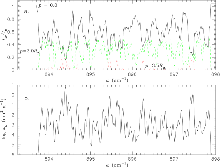
Figure 2: a: The spectra predicted by the P23n model at different impact parameters. The spectrum at the stellar disk center ($p=0.0$) is plotted with the solid line, while the spectrum at the extended wing ($p=3.5$ $R_{\rm p}$, see also Fig. 3) is plotted with the dotted line. The dashed line represents the spectrum between the above two cases, at $p=2.0$ $R_{\rm p}$. The contribution of the dust emission is not included in the spectra. b: The opacity of H₂O lines in an upper layer of the P23n model ($T=1020$ K and $\log P_{g}=-2.4$ dyn cm^-2). The spectra and the opacity are calculated with the HITEMP database. They are redshifted by 83 km s^-1 to match the observation and not convolved with a Gaussian representing the instrumental as well as macro-turbulent broadening.

The P23n model can also approximately predict the inverse P-Cyg profiles of strong H₂O lines observed at $\sim$894.9, 895.4, and 897.4 cm^-1, but there are still slight discrepancies in the line depths and positions. The model predicts the line profiles to be broader than those observed, and this appears to imply that the micro- and macro-turbulent velocities used in the calculation may be too large. However, while the use of smaller micro- and macro-turbulent velocities can improve the agreement with the observed line profiles of these strong H₂O lines, it also makes the weak and moderately strong H₂O lines much more conspicuous in the ISI bandpasses. Therefore, the difference in the line profiles may result from the uncertainties of the H₂O line data as well as the uncertainties of the atmospheric structure and/or the concept of constant, isotropic micro- and macro-turbulence itself. Figure 3 shows the intensity profiles predicted by the P23n model at $\sim$897.45 cm^-1 (on a strong H₂O line), 896.85 cm^-1 (in the “pseudo-continuum”), and in the true continuum, which was calculated with the H₂O line opacity set to zero. The intensity profile in the strong H₂O line (dotted line) shows a very extended wing with rather high intensities as compared to that in the pseudo-continuum (dashed line), which makes the line appear in emission above the pseudo-continuum.

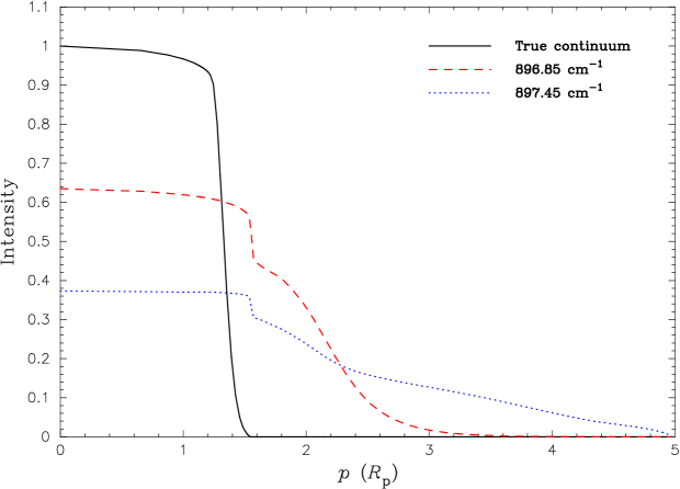
Figure 3: The intensity profiles in the true continuum (solid line), in the pseudo-continuum at 896.85 cm^-1 (dashed line), and in a strong H₂O line at 897.45 cm^-1 (dotted line) predicted by the P23n model. The intensity profiles are calculated with the HITEMP database and spectrally convolved to match the spectral resolution of the ISI measurements. The profiles are normalized with the value at $p=0$ of the intensity in the true continuum.

Figure 4 shows a comparison between the observed and synthetic spectra calculated with the P23n model in another wavelength region presented in WHT03a. The quality of the agreement with the observation is fair, though not fully satisfactory. The rather featureless spectrum observed in the region between 918.6 and 919.4 cm^-1 as well as between 901.2 and 902 cm^-1 is reproduced by the model to some extent, though the synthetic spectra tend to show too prominent spectral features. The strengths of the prominent H₂O lines at 918.2, 918.55, 902.0, and 902.37 cm^-1 are also in rough agreement, but there are still discrepancies between the observed line profiles and those predicted by the model.

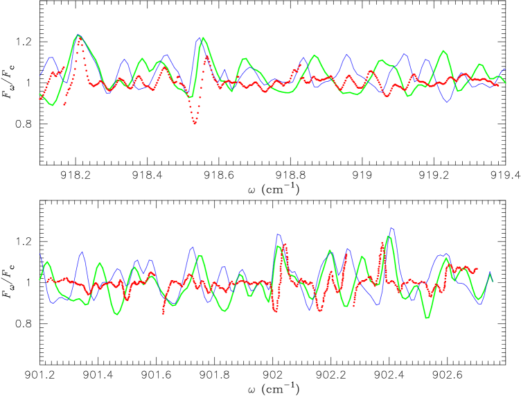
Figure 4: The synthetic spectra calculated with the P23n model are represented with the thick (HITEMP database) and thin (PS97 line list) lines. The observed spectrum is plotted with the dots. The synthetic spectra are redshifted by 83 km s^-1 to match the observation and already convolved with a Gaussian representing the macro-turbulence in the stellar atmosphere and the instrumental broadening.

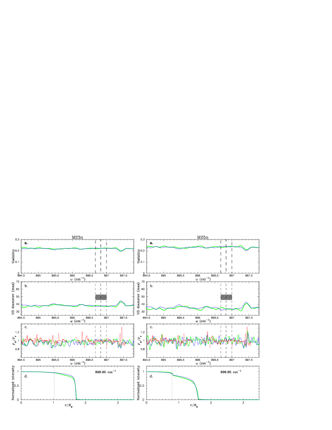
Figure 5: Comparison of the mid-infrared interferometric and spectroscopic observations with the predictions of selected M models. See also the caption to Fig. 1.

We found out that the other P models at phases later than 2.3 cannot reproduce the observed spectrum and uniform-disk diameters simultaneously: the 11 $\mu$m uniform-disk diameters are too small compared to the ISI measurements. The result obtained with the P24n model is shown in Fig. 1 (lower right) as an example. Obviously, this model predicts the 11 $\mu$m uniform-disk diameters to be considerably smaller than the observed values, while the synthetic spectra are in reasonable agreement with the observed spectrum. This results from the compactness of the atmospheres of the P models at phases later than 2.3, as compared to that of the P23n model.

3.2 M series

In this subsection, we discuss the spectra and the uniform-disk diameters predicted by the M models, which have a higher mass (1.2 $M_{\sun}$) than the P models (1.0 $M_{\sun}$). Figure 5 shows a comparison of the spectra and uniform-disk diameters calculated with the M23n and M25n models as examples. The visibilities and uniform-disk diameters plotted in the figure are derived for a projected baseline length of 30 m, as described in the previous subsection. The figure reveals that the M23n model can reproduce neither the observed 11 $\mu$m uniform-disk diameters nor the 11 $\mu$m spectrum. The predicted uniform-disk diameters are smaller than the ISI measurements, and the profiles of the strong H₂O lines (e.g., at 897.4 cm^-1) are in clear disagreement with the observation. The synthetic spectrum predicted by the M25n model is in rough agreement with the observation in the continuum-like part within the ISI bandpasses as well as in the profiles of the strong H₂O lines (for example, the lines at 897.4 cm^-1). However, the uniform-disk diameters calculated with this model are also much smaller than the observed values, as in the case of the M23n model. We note here, however, that the strong lines are formed in the uppermost layers and may be moderately affected by the fact that the model atmospheres are cut off at $5\times\mbox{$R_{\rm p}$}$ (see HSW98), and the transition to the circumstellar envelope is not taken into account.

It turned out that none of the M models considered here can simultaneously reproduce the observed 11 $\mu$m spectra and uniform-disk diameters. The atmospheres of the M models calculated for phases used in the present work are considerably more compact compared to those of the P models, which results in uniform-disk diameters much smaller than the observed values.

4 Discussion

The comparison of the model spectra and uniform-disk diameters with the TEXES and ISI observations discussed in the previous section demonstrates that the P23n model is the most appropriate one to explain the observations at phase 0.36. However, even this “best” model cannot provide fully satisfactory agreement with the observational results: the predicted uniform-disk diameters tend to be somewhat smaller than the observed values, and the synthetic spectra show too pronounced H₂O features.

One possibility to reconcile this discrepancy is to assume a flux contribution from the dust shell higher than that derived by WHT03a. They fitted the observed visibilities with two parameters, that is, the uniform-disk diameter and the fractional flux contribution of the stellar disk. However, as the intensity profiles plotted in Figs. 1 and 3 illustrate, uniform disks are not necessarily an appropriate approximation to characterize the real intensity distributions of Mira variables, and therefore, the dust flux contribution derived from the two-parameter fit may be affected by this assumption, even if the formal error of the fit is small.

We check the influence of the uncertainty of the flux contribution of the dust shell on the synthetic spectra and visibilities by changing $f_{\rm dust}$, the term representing the flux contribution of the dust shell. Figure 6 shows the result of calculations with the P23n model using three different values for $f_{\rm dust}$: 0.6, 0.7, and 0.8. The visibilities predicted at 896.85 cm^-1 are plotted as a function of spatial frequency, together with the ISI visibilities observed within the bandpass centered around 896.85 cm^-1. These ISI visibilities were obtained by binning the original calibrated visibilities of $o$ Cet measured on 2001 Dec. 19 at phase 0.36 (J. Weiner, M. J. Ireland, priv. comm.). The figure suggests that a flux contribution of the dust shell slightly higher than 0.7 can explain the observed visibilities. As the lower panel of the figure shows, an increase of the dust flux makes the H₂O features less pronounced, resulting in better agreement with the observed, continuum-like spectra. However, it also renders the strong H₂O lines (e.g., at 897.4 cm^-1) weaker, resulting in a poorer match with the observed line profiles. Thus, while the uncertainty of the flux contribution of the dust shell can be partially responsible for the discrepancy between the observations and the model, a mere change of $f_{\rm dust}$ is unlikely to solve the problem.

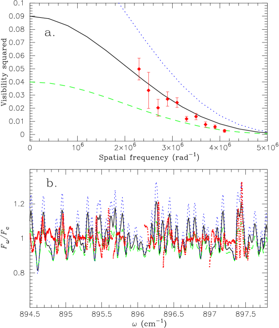
Figure 6: Comparison of the observed visibilities and spectra with those calculated with the P23n model using three different values for the fractional flux contribution of the dust shell. In both panels, the dotted, solid, and dashed lines represent the calculations with $f_{\rm dust}=0.6$, 0.7, and 0.8, respectively. a. The filled diamonds represent the ISI visibility points obtained at phase 0.36 (2001 Dec. 19). b. The 11 $\mu$m spectrum obtained with the TEXES instrument at phase 0.36 is plotted with the (red) dots.

Certainly, dynamical model atmospheres currently available cannot yet explain all observational aspects of Mira variables. A discrepancy between theory and observation can also be seen in the temporal variation of the spectral features. Weiner (weiner04 (2004)) presents high-resolution 11 $\mu$m spectra obtained at two different phases, 0.15 and 0.47, in the same cycle (see Fig. 4 in Weiner weiner04 (2004)). These spectra, which cover approximately the same wavelength range as we study here, exhibit only modest temporal variations, while the models predict much more pronounced changes between phase 2.2 and 2.4, as can be seen in Fig. 1.

It should be stressed here that there are numerous uncertainties of model parameters and modeling assumptions that may readily prevent good agreement between the observations and model predictions. For example, the only well-known stellar parameter of $o$ Cet is its period. The luminosity (and hence the effective temperature as well) derived from the observed bolometric flux and the star’s distance agrees with the model value for the Mira star R Leo, if the HIPPARCOS distance of Knapp et al. (knapp03 (2003)) is adopted (82 pc), whereas it is higher than the model value in the case of $o$ Cet (107 pc; see the discussion in ISW04, ISTW04, and Woodruff et al. woodruff04 (2004)). The uncertainty of the distance also directly affects the uniform-disk diameters predicted by the models. The mass of $o$ Cet (“around 1 $M_{\sun}$”, Wyatt & Cahn wyatt83 (1983)) and its metallicity are only a reasonable guess. Dynamical models covering a wider parameter range are being constructed but not yet available. Also, there are uncertainties in the treatment of physical processes included in the calculations of self-excited pulsation models and dynamical model atmospheres. Self-excited pulsation models may be moderately influenced by the treatment of convection. The numerous approximations adopted in the calculation of the time-dependent structure of the non-gray atmosphere as described in HSW98 may also be responsible for the discrepancy between the observations and model predictions. Note also that the H₂O line calculations presented here are performed with the assumption of LTE. Noticeable deviations from LTE may occur in the uppermost layers with low densities and affect particularly strong lines. For another molecule with strong features, TiO, M. J. Ireland et al. (in preparation) suggest that the strong TiO absorption bands are significantly affected by non-LTE effects.

One of the physical processes of great importance in understanding the structure of the outer atmosphere of Mira variables is the dust formation. Jeong et al. (jeong03 (2003)) present a detailed time-dependent hydrodynamic calculation for the oxygen-rich Mira variable IRC$-$20197 (IW Hya), which shows that the dust formation can take place at 3–5 $R_{\star}$. Although the parameters of IRC$-$20197 (lower effective temperature, higher luminosity, and higher mass loss rate compared to $o$ Cet) suggest that this object is much more evolved than $o$ Cet, the dust formation at such a vicinity of the star can also be expected in $o$ Cet. The formation of dust grains would have two effects on the comparison with the spectra and the angular size observed in the mid-infrared. Firstly, as discussed above, the flux contribution of the dust shell renders H₂O spectral features less pronounced. The derivation of uniform-disk diameters from visibilities measured at high spatial frequencies can also be affected for the following reason. That is, while the dust flux contribution appears as a steep visibility drop at low spatial frequencies if the dust shell lies well above the H₂O line-forming layers of the atmosphere, this is not the case if dust forms very close to the star and the dust shell is not well separated from the layers where H₂O lines form. In this case, the visibility function shows a more complex shape at low spatial frequencies (e.g., Lopez et al. lopez97 (1997)), which makes it difficult to derive reliably the uniform-disk diameters of the underlying atmosphere. Secondly, the dust formation in the upper layers can change the temperature and density stratifications due to the backwarming effect as well as dynamical effects resulting from the onset of mass outflows (e.g., Höfner et al. hoefner96 (1996); Bedding et al. bedding01 (2001); Jeong et al. jeong03 (2003)). In fact, a recent attempt to model the formation of dust grains and their effects on the atmospheric structure in the upper layers of the P and M models confirms that the dust formation does take place in those upper layers, but it also reveals serious problems in putting observational constraints on the details of the dust formation process (M. J. Ireland et al., in preparation).

5 Concluding remarks

We have presented a comparison of the mid-infrared spectra and angular sizes predicted by dynamical model atmospheres with the results of the TEXES and ISI observations. The P model in the second cycle calculated for a phase close to the observations can fairly reproduce the observed mid-infrared uniform-disk diameters and high-resolution spectra without introducing ad-hoc components. This result lends support to the picture obtained by semi-empirical models: the observed, continuum-like 11 $\mu$m spectra are the result of the filling-in effect due to the emission from extended water vapor layers, while these water vapor layers manifest themselves as an increase of the angular size from the near-infrared to the mid-infrared. On the other hand, the M models considered in the present work fail to reproduce the observed 11 $\mu$m uniform-disk diameters and the line profiles of prominent H₂O features, which can be attributed to their rather compact atmospheres at phases considered here.

Still, the “best” model in the P series (P23n) predicts the uniform-disk diameters at 11 $\mu$m to be somewhat smaller than the observed values. The predicted H₂O spectral features appear to be too pronounced and show too significant temporal variations compared to the observed spectra. These discrepancies may be attributed to the uncertainties of the input parameters such as the uncertainties of H₂O line data (line positions and line strengths), the unknown stellar mass and/or luminosity, as well as those of the treatment of relevant physical processes. From the density and temperature conditions in the extended configurations of the P and M models, we also suspect that dust formation may occur in the upper atmospheric layers. More refined dynamical models (with dust formation) would be needed to obtain a definitive explanation for the increase of the angular diameter from the near-infrared to the mid-infrared as well as the flat mid-infrared spectra observed in Mira variables.

- (1) Bedding, T., Jacob, A. P., Scholz, M., & Wood, P. R. 2001, MNRAS, 325, 1487
- (2) Bessell, M., Scholz, M., & Wood, P. R. 1996, A&A, 307, 481
- (3) Danchi, W. C., Bester, M., Degiacomi, C. G., Greenhill, L. J., & Townes, C. H. 1994, AJ, 107, 1469
- (4) Fedele, D., Wittkowski, M., Paresce, F., et al. 2005, A&A, 431, 1019
- (5) Hinkle, K. H., & Barnes, T. G. 1979, ApJ, 227, 923
- (6) Hofmann, K.-H., Scholz, M., & Wood, P. R. 1998, A&A, 339, 846 (HSW98)
- (7) Höfner, S., Fleischer, A. J., Gauger, A., et al. 1996, A&A, 314, 204
- (8) Ireland, M. J., Tuthill, P. G., Bedding, T. R., Robertson, J. G., & Jacob, A. P. 2004a, MNRAS, 350, 365
- (9) Ireland, M. J., Scholz, M., & Wood, P. R. 2004b, MNRAS, 352, 318 (ISW04)
- (10) Ireland, M. J., Scholz, M., Tuthill, P. G., & Wood, P. R. 2004c, MNRAS, 355, 444 (ISTW04)
- (11) Ireland, M. J., Tuthill, P. G., Davis, J., & Tango, W. 2005, MNRAS, 361, 337
- (12) Jeong, K. S., Winters, J. M., Le Bertre, T., & Sedlmayr, E. 2003, A&A, 407, 191
- (13) Jones, H. R. A., Pavlenko, Y., Viti, S., & Tennyson, J. 2002, MNRAS, 330, 675
- (14) Knapp, G. R., Pourbaix, D., Platais, I., & Jorissen, A. 2003, A&A, 403, 993
- (15) Lacy, J. H., Richter, M. J., Greathouse, T. K., Jaffe, D. T., & Zhu, Q. 2002, PASP, 114, 153
- (16) Lopez, B., Danchi, W. C., Bester, M., et al. 1997, ApJ, 488, 807
- (17) Mennesson, B., Perrin, G., Chagnon, G., et al. 2002, ApJ, 579, 446
- (18) Mihalas, D. 1978, Stellar Atmospheres, 2nd edition, San Francisco, W. H. Freeman and Co.
- (19) Millan-Gabet, R., Pedretti, E., Monnier, J. D., et al. 2005, ApJ, 620, 961
- (20) Ohnaka, K. 2004b, A&A, 421, 1149
- (21) Ohnaka, K. 2004a, A&A, 424, 1011
- (22) Ohnaka, K., Bergeat, J., Driebe, T., et al. 2005, A&A, 429, 1057
- (23) Partridge, H., & Schwenke, D. W. 1997, J. Chem. Phys., 106, 4618 (PS97)
- (24) Perrin, G., Ridgway, S. T., Coudé du Foresto, V., et al. 2004, A&A, 418, 675
- (25) Rothman, L. S. 1997, HITEMP CD-ROM (Andover: ONTAR Co.)
- (26) Scholz, M., & Wood, P. R. 2000, A&A, 362, 1065
- (27) Schuller, P., Salomé, P., Perrin, G., et al. 2004, A&A, 418, 151
- (28) Tej, A., Lançon, A., & Scholz, M. 2003a, A&A, 401, 347
- (29) Tej, A., Lançon, A., Scholz, M., & Wood P. R. 2003b, A&A, 412, 481 (TLSW03)
- (30) Tevousjan, S., Abdeli, K.-S., Weiner, J., Hale, D. D. S., & Townes, C. H. 2004, ApJ, 611, 466
- (31) Weiner, J. 2004, ApJ, 611, L37
- (32) Weiner, J., Danchi, W. C., Hale, D. D. S., et al. 2000, ApJ, 544, 1097 (W00)
- (33) Weiner, J., Hale, D. D. S., & Townes, C. H. 2003a, ApJ, 588, 1064 (WHT03a)
- (34) Weiner, J., Hale, D. D. S., & Townes, C. H. 2003b, ApJ, 589, 976 (WHT03b)
- (35) Wood, P. R., Alcock, C., Allsman, R. A., et al. 1999, In: Asymptotic Giant Branch Stars, IAU Symp. 191, eds. T. Le Bertre, A. Lèbre, & C. Waelkens, p.151
- (36) Woodruff, C., Eberhardt, M., Driebe, T., et al. 2004, A&A, 421, 703
- (37) Wyatt, S. P., & Cahn, J. H. 1983, ApJ, 275, 225