Large scale correlations in galaxy clustering from the Two degree Field Galaxy Redshift Survey

We study galaxy correlations from samples extracted from the 2dFGRS final release. Statistical properties are characterized by studying the nearest neighbor probability density, the conditional density and the reduced two-point correlation function. The result is that the conditional density has a power-law behavior in redshift space described by an exponent $\gamma=0.8\pm 0.2$ in the interval from about 1 Mpc/h, the average distance between nearest galaxies, up to about 40 Mpc/h, corresponding to radius of the largest sphere contained in the samples. These results are consistent with other studies of the conditional density and are useful to clarify the subtle role of finite-size effects on the determination of the two-point correlation function in redshift and real space.

1 Introduction

The problem of the quantitative characterization of the large scale galaxy clustering has been intensively discussed in the last years, especially in relation to two new galaxy surveys: the Sloan Digital Sky Survey (SDSS — York et al., 2000) and the Two degree Field Galaxy Redshift Survey (2dFGRS — Colless et al., 2003). These data represent a great improvement for our knowledge of the local universe: for example the number of measured redshifts has grown of a factor ten with respect to the surveys completed in the last two decades. Moreover accurate redshift determinations and the multi-bands photometry allow one a precise characterization of many parameters and effects (e.g. K corrections) which were poorly constrained up to few years ago. It should however be noted that for some analyses, like the ones we discuss here, a large solid angle is also required. This is still not the case for the present data, but, for instance, the final release of the SDSS will provide a large contiguous angular sky region in the very near future.

In this paper we discuss the analysis of two-point correlation properties in the 2dFGRS sample. Up to now these data were mainly analyzed by studying the reduced correlation function $\xi(r)$, in redshift and real space, and its Fourier conjugate, the power spectrum (e.g. N‘orberg et al. 2001, 2002; Tegmark, Hamilton & Xu 2002; Hawkins et al. 2003; Madgwick et al. 2003, Basilakos & Plionis 2003, Cole et al. 2005). Recently Gaztanaga et al. (2005) present new result for the 3-point correlation function measured as a function of scale, luminosity and color using the 2dFGRS sample.

In general, these statistical tools can be affected by finite-size effects or luminosity dependent selection effects (e.g. Gabrielli et al., 2004) and, by using appropriate statistics, one may perform several tests in order to disentangle different biases. Finite size effects can be very important for the determination of correlation properties in the regime of large fluctuations, which should be then clearly identified in the studies of galaxy samples. It is in fact well known that at small scales, observed galaxy structures are highly irregular and present two-point power-law correlations, in the regime of strong clustering. However the search for the “maximum” size of galaxy structures and voids, beyond which the distribution becomes essentially uniform and fluctuations can be considered small perturbations with respect to the average density, is still an open problem (Tikhonov & Makarov 2003, Hogg et al. 2005, Joyce et al. 2005 and see for a recent review Baryshev & Teerikorpi 2005). It is evident that from the theoretical point of view the understanding of the statistical characteristics of these structures represents the key element to be considered by a physical theory dealing with their formation.

A number of statistical methods can be used to study galaxy distribution, the main ones involve the determination of two-point properties although the study of the distribution function, containing information on higher order correlations, has also been found to be a powerful method (e.g. Sivakoff & Saslaw 2005). The primary questions in correlation analysis of three dimensional galaxy distributions are: (i) what is the value of the correlation exponent and (ii) which is the scale where the distribution becomes uniform and a crossover to homogeneity can be clearly identified ? Such a scale can be defined, for example, to be the one beyond which conditional counts of galaxies in three dimensional volumes of radius $R$ grow as $R^{3}$. Recently Hogg et al. (2005), by considering the properties of a deep and complete sample of luminous red galaxies extracted from the SDSS survey, found that the transition from the strongly correlated regime to the uniform one occurs at about 70 Mpc/h, which is larger than, for example, results in the CfA1 redshift survey where the transition was found at about 20 Mpc/h (Davis & Peebles, 1983; see Peebles 2001 for a recent discussion). Particularly, they have measured the behavior of the conditional density in redshift space, finding that the exponent characterizing power law correlation is about $\gamma\approx 1$ (instead of $\gamma=1.8$ as measured by Davis & Peebles 1983) up to 20-30 Mpc/h and that this is followed by a slow crossover toward homogeneity which is reached at about 70 Mpc/h. These results are in good agreement with the ones presented in, e.g. Sylos Labini et al. (1998) (see Baryshev & Teerikorpi, 2005 for a recent review) where the same value $\gamma\approx 1$ was found up to 20-30 Mpc/h and where at larger scales, with a weaker statistics, an evidence for a compatibility with the extension of such a behavior was found. In addition Tikhonov, Makarov & Kopylov (2000) found similar results up to scales of $\sim 30$ Mpc/h, and weaker evidences for homogeneity at scales larger than 100 Mpc/h.

In this paper we present results of a correlation analysis of the 2dFGRS data studying the behavior of the conditional density and other statistics suitable to characterize properties of distributions with large fluctuations and control finite size effects. In Sec.2 we describe the procedure to construct samples which are not biased by the luminosity selection in apparent magnitudes (the so-called volume limited — VL — samples). In Sec.3 we consider the nearest neighbor probability density for the VL samples which allows us a characterization of small scales statistical properties. We then turn to the study of large scale in Sec.4 where we discuss the estimation of the conditional density and the result obtained in the VL samples. We discuss the relation of this statistical tool with the reduced two-point correlation function in Sec.5, where we compare our results with previous estimations of the same statistics, focusing on finite size effects and their implication for the interpretation of galaxy correlations. Finally in Sec.6 we summarize our results and discuss its relation to other studies and we draw our main conclusions.

2 Volume limited subsamples

The 2dFGRS is the largest galaxy catalog completed at the moment. The Final Release (Colless et al., 2003) contains more than $220$ thousands of precisely measured redshifts of the galaxies located in two strips: about $140$ thousands in the southern galactic pole (SGP), in a strip of $90^{\circ}\times 15^{\circ}$ and about $70$ thousands in the strip $75^{\circ}\times 10^{\circ}$ in northern galactic pole (NGP) In addition the survey contains $10$ thousands in the random fields which are not used in this paper.

The median redshift of galaxies is $z\simeq 0.1$ and most of the galaxies have $z<0.3$. The $b_{J}$ magnitude corrected for the galactic extinction is limited as $14.0<b_{J}<19.45$.

2.1 Selection of subsamples

To avoid the effect of the irregular edges in the angular coordinates, due to the survey geometry, we set the following limits in right ascension and declination in order to get rectangular (in $\alpha,\,\delta$ coordinates) shape on the sky:

• SGP: $84^{\circ}\times 9^{\circ}$ ($-33^{\circ}<\delta<-24^{\circ}$, $-32^{\circ}<\alpha<52^{\circ}$)

• NGP: $60^{\circ}\times 6^{\circ}$ ($-4^{\circ}<\delta<2^{\circ}$, $150^{\circ}<\alpha<210^{\circ}$)

We select galaxies in the redshift interval $0.01\leq z\leq 0.3$ and with redshift quality parameter such that $Q\geq 3$ in order to have high quality redshifts (see discussion in Hawkins et al. 2003).

We do not use a correction for the redshift completeness mask and for the fiber collision effects. In fact, completeness varies mostly nearby the survey edges which are excluded in our sample. We assume that fiber collisions do not make a sensible change in the small scales correlation properties as we set our lower cut-off to 0.5 Mpc/h which is larger than 0.1 Mpc/h used by Hawkins et al. (2003).

To construct VL subsamples first we compute metric distances as

$$r(z)=\frac{c}{H_{0}}\int_{\frac{1}{1+z}}^{1}{\frac{dy}{y\cdot\left(\Omega_{M}/y+\Omega_{\Lambda}\cdot y^{2}\right)^{1/2}}}\leavevmode\nobreak\ ,$$ (1)

where we use the standard model parameters $\Omega_{M}=0.3$ and $\Omega_{\Lambda}=0.7$. The absolute magnitude can be computed as

$$M=b_{J}-5\cdot\log_{10}\left[r(z)\cdot(1+z)\right]-K_{i}(z)-25.$$ (2)

To calculate the K-correction $K_{i}(z)$ (the index $i$ defines the galaxy type) we used formulas obtained by Madgwick et al. (2002):

$$\begin{array}[]{lcl}K_{1}(z)&=2.6z+4.3z^{2}&\mbox{(E/S0)}\\ K_{2}(z)&=1.9z+2.2z^{2}&\mbox{(Sa/Sb)}\\ K_{3}(z)&=1.3z+2.0z^{2}&\mbox{(Sc/Sd)}\\ K_{4}(z)&=0.9z+2.3z^{2}&\mbox{(Irr)}\\ K_{avg}(z)&=1.9z+2.7z^{2}&\mbox{(average)}\\ \end{array}$$ (3)

where $1,2,3,4$ indexes represent the spectral types of the galaxies (in parenthesis in Eq.3), and the average value $K_{avg}(z)$ is used for the galaxies with the undefined spectral type.

2.2 Definition of volume limited subsamples

To take into account the selection effect that arises due to the 2dFGRS apparent magnitude limits $14<b_{J}<19.45$, one has to consider two limits for the metric distance $r_{min}<r<r_{max}$ and compute the two corresponding limits for the absolute magnitude $M_{min}(r_{min})$ and $M_{max}(r_{max})$ which represent the lower and the upper limit for the galaxies contained in a VL sample.

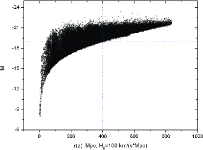
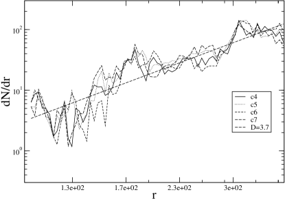
To this aim, we select three distance intervals (50-250 Mpc/h, 100-400 Mpc/h and 150-550 Mpc/h) and compute the corresponding absolute magnitude limits for each of two strips. Thus we get three VL subsamples for the Northern hemisphere and three for Southern hemisphere whose main parameters are presented Table 1. (Note that hereafter we set $h=1$ unless specified). An example of the distance-magnitude limits for the SGP400 sample (which indeed is the largest one considered in this paper) is shown in Fig. 1. In Fig 2 we show the behavior of the differential number counts $dN(r)/dr$ as a function of distance in different sky areas for the sample SGP400. Particularly we put limits respectively at $\delta\leq-27^{\circ}$ (c4), $\delta>-27^{\circ}$ (c5), $\alpha\geq 189^{\circ}$ (c6) and $\alpha\geq 189^{\circ}$ (c7). As an example we report the best fit for the sample c4, which show an exponent corresponding to a metric dimension larger ($D=3.7$) than the space dimension. This is a purely finite-size effect corresponding to the large fluctuations still visible at scales of order 100 Mpc/h.

Figure 1: The metric distance- absolute magnitude diagram for the SGP strip. The boundaries of the SGP400 subsample are shown.

Figure 2: Differential number counts in different sky areas (defined in the text) for the SGP400 subsample. As an example we report the best fit for the sample c4, which show an exponent corresponding to a metric dimension larger than the space dimension. This is a purely finite-size effect which maybe explained by a presence of the large scale fluctuations in the studied region.

VL sample	$r_{min}$	$r_{max}$	$M_{min}$	$M_{max}$	$N_{g}$
SGP250	50	250	-19.5	-17.8	14177
SGP400	100	400	-20.8	-19.0	29373
SGP550	150	550	-21.2	-19.8	26289
NGP250	50	250	-19.5	-17.8	12474
NGP400	100	400	-20.8	-19.0	23208
NGP550	150	550	-21.2	-19.8	18030

Table 1: Main properties of the obtained VL samples: $r_{min}$, $r_{max}$ are the chosen limits for the metric distance; ${M_{min},\,M_{max}}$ are the interval for the absolute magnitude and $N_{g}$ is the resulting number of galaxies in each sample.

3 Nearest neighbor probability density

In a stochastic point process the probability $\omega(r)dr$ that the nearest neighbor to a given particle lies at a distance in the range $[r,r+dr]$ can provide a useful characterization of small scale statistical properties. This probability density satisfies, by definition, the condition

$$\int_{0}^{\infty}{\omega(r)dr}=1.$$ (4)

According to its definition $\omega(r)$ can be simply estimated as

$$\omega_{E}(r)=N_{nn}(r)/\left(\int_{0}^{\infty}{N_{nn}(r^{{}^{\prime}})dr^{{}^{\prime}}}\right),$$ (5)

where $N_{nn}(r)$ is the number of points which have their nearest neighbors in the range $[r,r+dr]$.

The nearest neighbor probability density for a Poisson distribution with average density $\langle{n}\rangle$, is given by (Gabrielli et al. 2004)

$$\omega(r)=4\pi\langle{n}\rangle{r^{2}}\exp\left(-\frac{4\pi\langle{n}\rangle{r^{3}}}{3}\right).$$ (6)

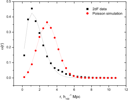
In Fig. 3 we present an example of the observed $\omega(r)$ distribution in the VL SGP400, along with an artificial Poisson distribution with the same number of points in the same three-dimensional volume. Note that the probed scales here are about $0.1\div 10$ Mpc/h.

For the actual data the average distance between nearest galaxies is smaller than for the Poisson case, and this is a clear evidence of the presence of small scale correlations. The exact analytical behavior of $\omega(r)$ for the general case of a power-law correlated structure is unknown; an approximate relation for the simple case of a anisotropic Poisson distribution, which present a radial density profile decaying as $n_{c}(r)\sim r^{-\alpha}$ from its center with exponent $\alpha$ (with $\alpha>1.5$ — see discussion in Gabrielli et al. 2004), is given by

$$\omega(r)=4\pi C{r^{2-\gamma}}\exp\left(-\frac{4\pi C}{3-\gamma}r^{3-\gamma}\right)\;,$$ (7)

where $\gamma=3-2\alpha$. This is found to be a good approximation in the actual data (see Fig.1). In Tab.2 (see below) we report the estimation of the average distance between nearest neighbors (defined as $r_{sep}=\int r\omega(r)dr$) in the different samples (Note that similar values have been found by Peebles 2001).

Figure 3: Nearest neighbor probability density for the SGP400 sample data (squares) and for a Poisson simulation (circles) in the same volume. The dotted lines are the best fit respectively for the anisotropic Poisson distribution (Eq.7 with $\gamma=1.2$) and for the Poisson case (Eq.6).

4 Estimation of correlations: the conditional density

In general, in a distribution of points with large fluctuations at some scales, one may determinate two-point correlations through the estimation of the conditional density (see discussion in Gabrielli et al. (2004)). We first briefly summarize the main properties of this statistical tool stressing the finite size effects and statistical errors which may enter into the estimators. Then we apply it to the case of the VL samples extracted from the 2dFGRS, as discussed in the previous section.

4.1 Conditional density in spheres $\Gamma^{*}(r)$

The conditional density in spheres $\Gamma^{*}(r)$ is defined for an ensemble of realizations of a given point process, as

$$\Gamma^{*}(r)=\frac{\langle{N(r)}\rangle_{P}}{\|C(r)\|}.$$ (8)

This quantity measures the average number of points $\langle{N(r)}\rangle_{P}$ contained in a sphere of volume $\|C(r)\|=\frac{4}{3}\pi{r}^{3}$ with the condition that the center of the sphere lies on an occupied point of the distribution (and $\langle{...}\rangle_{P}$ denotes the conditional ensemble average).

Such a quantity can be estimated in a finite sample by a volume average (supposing stationarity of the point distribution)

$$\Gamma^{*}_{E}(r)=\frac{\overline{N(r)}_{P}}{\|C(r)\|}=\frac{1}{N_{c}(r)}\sum_{i=1}^{N_{c}(r)}{\frac{N_{i}(r)}{\|C(r)\|}},$$ (9)

where $N_{c}(r)$ — the number of points (centers) with balls fully contained in the sample volume, $\overline{(...)}_{P}$ means averaging by the sample points.

Given a sample of arbitrary geometry and a scale $r$ at which correlations are measured, only a subsample of the points contained in it will satisfy the following requirement: when chosen as center of a sphere of radius $r$, the sphere is fully contained in the sample volume. When the average in Eq.9 is made over such a subsample one is considering the full-shell estimator of the conditional density. Note that the number of center $N_{c}(r)$ is a function of the scale $r$ at which correlations are estimated. In fact for scales much smaller than the radius $r_{s}^{m}$ of the largest sphere fully contained in the sample volume, almost all points will contribute to the average, while at scales comparable to the sample size only those points lying in the center of the sample volume will contribute. Thus finite-size effect can be important when one considers the largest available scales: in this situation one cannot make a full volume average and systematic effect, due to large fluctuations, can be important in the determination of such a statistics.

The scale $r_{s}^{m}$ will in general be very different from the scales $r_{min}$ and $r_{max}$ characterizing a VL sample, as it depends crucially on the sample solid angle. On the other hand the minimal scale $r_{sep}$ up to which correlations can be measured, is given by the average distance between neighbor galaxies: clearly for $r<r_{sep}$ discrete shot-noise dominates estimations of any statistical quantity. Thus we will explicitly compute the scales $r_{sep}$ and $r_{s}^{m}$ for the VL considered in what follows (see Tab.2).

4.2 Conditional density in shells $\Gamma(r)$

The conditional density in spherical shells is defined as

$$\Gamma(r)=\frac{\langle{N(r,\Delta{r})}\rangle_{P}}{\|C(r,\Delta{r})\|},$$ (10)

where $\langle{N(r,\Delta{r})}\rangle_{P}$ represents the ensemble average number of points in a sphere of radius $r$ and thickness $\Delta{r}$, of volume $\|C(r,\Delta{r})\|=\frac{4}{3}\pi[(r+\Delta{r})^{3}-r^{3}]$, around a point of distribution (and thus this is a conditional ensemble average $\langle{...}\rangle_{P}$ as in the previous case). Note that one can also write Eq.10 as

$$\Gamma(r)=\frac{\langle{n(r)n(0)}\rangle}{\langle{n(0)}\rangle}$$ (11)

where $\langle...\rangle$ represents the (unconditional) ensemble average and $n(r)$ is the microscopic number density.

The conditional density in shells can be estimated in a finite sample by the following volume average

$$\Gamma_{E}(r)=\frac{\overline{{N(r,\Delta{r})}}_{P}}{\|C(r,\Delta{r})\|}=\frac{1}{N_{c}(r+\Delta{r})}\sum_{i=1}^{N_{c}(r+\Delta{r})}{\frac{{N_{i}}(r,\Delta{r})}{\|C(r,\Delta{r})\|}},$$ (12)

where we consider again only the full-shell estimator, i.e. for which $N_{c}(r+\Delta{r})$ represents the number of points (centers) contained in spherical shells fully contained in the sample volume. Analogously to the case of $\Gamma^{*}(r)$ particular care should be used to determine the scales $r_{sep}$ and $r_{s}^{m}$.

It is instructive to notice that for the case where the distributions has power-law correlations and strong fluctuations (e.g. a fractal structure) then the conditional density in spheres behaves (in the ensemble average) as

$$\Gamma^{*}(r)=\frac{3B}{4\pi}\leavevmode\nobreak\ r^{-\gamma}\,,$$ (13)

while conditional density in shells has the form

$$\Gamma(r)=\frac{(3-\gamma)B}{4\pi}\leavevmode\nobreak\ r^{-\gamma}.$$ (14)

where $\gamma$ is the correlation exponent (in the case of a fractal $D=3-\gamma$ is the fractal dimension) and $B$ is a lower cut-off related to the smaller scale where correlation can be measured in a finite sample (i.e. to $r_{sep}$ previously defined).

4.3 Application to 2dFGRS data

In Tab.2 we show, for the different VL samples considered, the lower and upper cut-off, previously discussed, between which we have estimated $\Gamma(r)$ and $\Gamma^{*}(r)$. Note that we have generated a Poisson distribution, for each VL sample, with the same number of points and in the same three dimensional volume in order to estimate the same statistical quantities in a distribution without correlation at all. This provide us with a useful way to test our analysis with the simplest distribution with known properties. Note also that all our estimates have been done in redshift space: the relation with real space properties will be discussed in Sec.6.

VL sample	$r_{sep}$, 2dFGRS	$r_{sep}$, Poisson	$r_{s}^{m}$
NGP250	1.3	2.0	12.4
NGP400	1.7	2.6	19.9
NGP550	2.7	3.9	27.4
SGP250	1.5	2.4	18.2
SGP400	1.9	3.0	29.1
SGP550	2.8	4.2	40.0

Table 2: Characteristic scales of the VL samples: $r_{sep}$ is the average separation distance between nearest neighbor galaxies (in 2dFGRS and Poisson distribution within the same volume and for the same number of galaxies), $r_{s}^{m}$ is the maximum sphere completely contained in the sample. All distances are in Mpc ($H_{0}=100$ km/sec/Mpc).

Fig.4

Figure 4: Estimation of the conditional density in spheres in the six VL samples considered (different symbols correspond to different VL samples — see labels). The reference line has a power-law behavior with slope $\gamma=0.8$.

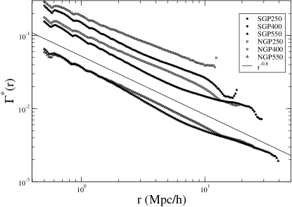
shows the behavior of the estimation of the conditional density in spheres in the six VL samples considered. It is interesting to note that samples with same luminosity and distance cuts in the NGP and SGP show approximately the same behavior. However a difference in the amplitude is present for all but the largest sample. The amplitude of $\Gamma^{*}(r)$ is related to the luminosity function in the following way.

In general one has that the joint conditional probability of finding a galaxy of luminosity $L$ at distance $\@vec{r}$ from another galaxy, i.e. the (ensemble) conditional average number of galaxies with luminosity in the range $[L,L+dL]$ and in the volume element $d^{3}r$ at distance $r$ from an observer located on a galaxy is given by $\langle\nu(L,\@vec{r})\rangle_{p}d^{3}rdL$. One can then assume that

$$\langle\nu(L,\@vec{r})\rangle_{p}=\phi(L)\times\Gamma(r)\;,$$ (15)

where $\Gamma(r)$ is the average conditional density and $\phi(L)$ is the luminosity function such that $\phi(L)dL$ gives the probability that a randomly chosen galaxy has luminosity in the range $[L,L+dL]$. By writing Eq.15 as a product of the conditional space density for the luminosity function, one has implicitly assumed that galaxy positions are independent of galaxy luminosity. Thus from Eq.15 it follows that the amplitude of $\Gamma^{*}(r)$ in a VL sample is given by an integral of the luminosity function over the range of absolute luminosity covered by the sample multiplied by the conditional density for all galaxies. Amplitude variations in the same VL samples in the NGP and SGP can be due to large local fluctuations which are not averaged out by the volume average. Thus these differences can be probably ascribed to finite size effects. The fact that in the deepest VL samples (i.e. the ones cut at 550 Mpc/h), where the volume is the largest, the conditional density does not show significant differences between the two hemispheres supports the finite-size interpretation.

If one fits the behavior of the estimated $\Gamma^{*}(r)$ with a power-law function of the type $Br^{-\gamma}$ one finds that $\gamma=0.8\pm 0.2$. In Fig.5

Figure 5: Conditional density is spheres normalized to the value at 10 Mpc/h In this way it is apparent the fact that the slope variates in the different samples. The reference line has a power-law behavior with slope $\gamma=0.8$.

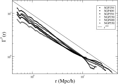
we have normalized the conditional density is spheres to the value at 10 Mpc/h. In this way it is apparent the fact that the slope variates in the different samples: the variation is of about 0.1. The formal statistical error for the determination of $\Gamma^{*}(r)$ at each scale can be simply derived from the dispersion of the average

$$\Sigma^{2}(r)=\frac{1}{N}\sum_{i=1}^{N-1}\frac{\left(\Gamma_{i}^{*}(r)-\Gamma^{*}(r)\right)^{2}}{N-1}$$ (16)

where $\Gamma_{i}^{*}(r)$ represents the determination from the $i^{th}$ point. The corresponding error bars are too small to be plotted. However one should notice that at large scales (usually the last few points) estimators of $\Gamma^{*}(r)$ have large scatterings because of the small number of points contributing to the average. Moreover in this estimation one cannot take into account systematic variations due to the fact that the volume average cannot be performed at large scales (see discussion in Joyce, Montuori & Sylos Labini 1999). For these reasons the behavior for scale larger than $\sim 20$ Mpc/h is affected by large un-averaged fluctuations.

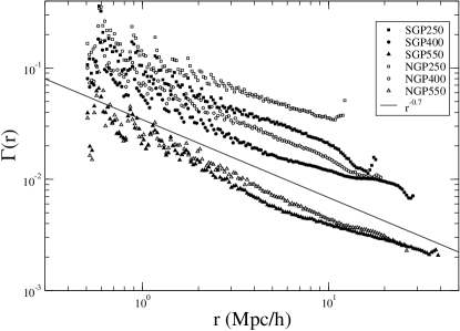
We show in Fig.6 the behavior of the conditional density in shells and in Fig.7 the conditional density in shells normalized to the value at 10 Mpc/h. It is clear that these estimations are more affected by statistical noise. An important parameter in this respect is represented by the shell thickness which we take constant in logarithmic scale.

Figure 6: Estimation of the conditional density in shells for the different VL samples considered. The reference line has a power-law behavior with slope $\gamma=0.7$.

Figure 7: Estimation of the conditional density in shells normalized to the value at 10 Mpc/h for the different VL samples considered. The reference line has a power-law behavior with slope $\gamma=0.7$.

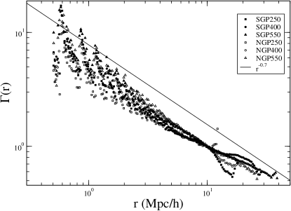
In this case the average slope is $\gamma=0.8\pm 0.2$ up to 30 Mpc/h.

5 Estimation of the reduced two-point correlation function

The reduced two-point correlation function $\xi(r)$ for a stochastic point process is defined (see e.g. Peebles, 1980) as

$$\xi(r)=\frac{\langle{n(r)n(0)}\rangle}{\langle{n(0)}\rangle^{2}}-1=\frac{\Gamma(r)}{\langle{n}\rangle}-1,$$ (17)

where $\langle{...}\rangle$ indicates the ensemble average and $\langle{n}\rangle$ — is the ensemble average number density. The last equality follows from the very definition of the conditional density (see Eq.10).

There are several estimators of $\xi(r)$ and we refer to Kerscher, Szapudi & Szalay (2000) and Gabrielli et al. (2004) for a detailed discussion of the different ones used in the literature. One may consider, for example, the Landy & Szalay (1993) (LS) estimator that is the most widespread in modern studies of correlation function for large scale structures because it is the minimal variance estimator for a Poisson distribution. This can be written as (Kerscher, Szapudi & Szalay al. 2000):

$$\xi_{LS}(r)=\frac{N_{R}(N_{R}-1)}{N_{D}(N_{D}-1)}\frac{DD(r)}{RR(r)}-2\frac{N_{R}-1}{N_{D}}\frac{DR(r)}{RR(r)}+1,$$ (18)

where $N_{D}$ — the number of data (sample) points; $N_{R}$ — the number of random points homogeneously distributed in the sample geometry; $DD(r)$ is the number data-data pairs, $DR(r)$ — data-random pairs and $RR(r)$ — random-random pairs respectively. Note that in the artificial random catalogs generated for the estimation of Eq.18, we have used a number points in the range 4.5-9$10^{4}$. However the LS estimator can be biased by finite-size effects in the case of strongly correlated distributions as we discuss in what follows:we have tested that also for the estimator introduced by Davis & Peebles (1983) the situation is substantially the same.

Analogously to the full-shell estimator of the conditional density, one may define the following (full-shell) estimator of $\xi(r)$ which can be induced directly from Eq.17

$$\xi_{FS}(r)=\frac{\Gamma_{E}(r)}{\Gamma^{*}_{E}(r_{s}^{m})}-1\;.$$ (19)

where $\Gamma_{E}(r)$ is the estimator of the conditional density in shells and $\Gamma^{*}_{E}(r_{s}^{m})$ is the estimator of the conditional density in spheres at the scale of the sample $r_{s}^{m}$. Although the latter quantity is not, in general, computed through an average because only a single point may contribute at such large scales, this estimator, when the properties of the distribution are unknown and likely to be characterized by strong fluctuations, has several advantages with respect to the LS (or also the one used by Davis & Peebles, 1983).

We notice that by using the full-shell estimator we are able to make a very conservative measurement of the two-point correlation function. In fact, for example, one does not need to make estimations of correlations on scales larger than $r_{s}^{m}$ which require use of weighing schemes and special treatment of boundary conditions. The main point is however that the estimation of the sample density is performed on “local” scales, i.e. much smaller than the global scale of the sample. In addition Eq.19 satisfies the simple constraint

$$\int_{0}^{r_{s}^{m}}\xi_{FS}(r)r^{2}dr=0$$ (20)

which is the so-called “integral constraint”. Any estimator of $\xi(r)$ must satisfy a similar condition which comes from the fact that the average density has been estimated from the given sample. (Note that we do not use any additional correction to take into account for this particular effect: in the case of the full-shell estimator the integral constraint has a clear effect given by Eq.20. For the case of the LS estimator we have not used any correction to take into account for this constraint.) It is however clear that Eq.20 gives us a simple way of controlling this offset, which is not the case for another estimator. It is important to stress that the estimation of the sample average is subjected to large fluctuations because its determination does not involve any average. Such fluctuations will substantially alter the amplitude of the reduced correlation function as we discuss below: this is a good reason to measure statistical quantities, like $\Gamma(r)$, which are not affected by such fluctuations.

The behavior of $\xi_{FS}(r)$ is presented on Fig. 8.

Figure 8: Estimation of the two-point reduced correlation function in the different VL samples considered by using the full shell estimator. The reference line has a power-law behavior with slope $\gamma=0.75$.

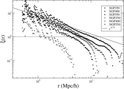
We note two main properties: the first one is that the amplitude of $\xi(r)$ changes in different samples and the second is that the exponent in the strongly clustered regime (i.e. $\xi(r)\gg 1$) is about $\gamma=0.75$. Both results are in qualitative agreement with other analysis of the same samples. For example Hawkins et al. (2003) found that in the full magnitude limited sample, the redshift space value of the correlation exponent is $\gamma=0.75$ in the range [0.1,4] Mpc/h and then $\gamma=1.75$ in the range [4,10] Mpc/h (see their Fig.6). This is for example what we find in the SGP250 sample as shown in Fig.9. It is worth noticing that the slopes measured in different VL sample may variate as it is shown, for example, by the SGP400 in Fig.10.

Figure 9: Estimation of the two-point reduced correlation function in the VL sample SGP250, by using the full shell estimator. The reference lines have a power-law behavior with slope $\gamma=0.75$ and $\gamma=1.57$ respectively.

Figure 10: Estimation of the two-point reduced correlation function in the VL sample SGP400, by using the full shell estimator. The reference lines have a power-law behavior with slope $\gamma=1.0$ and $\gamma=1.7$ respectively.

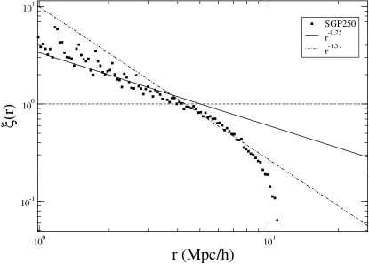
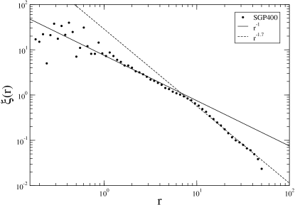
It is interesting to note that in other surveys different values of $\gamma$, in redshift space, have been found: for example in the CfA1 catalog $\gamma=1.8$ in the range [0.1,5] Mpc/h (Davis & Peebles 1983). As discussed below we ascribe this change of slope, as the variation of the amplitude of $\xi(r)$, to a finite size effect. For this reason, while the qualitative behavior of the variation of the amplitude and exponent of $\xi(r)$ is similar to many other estimations (e.g. Hawkins et al., 2003; Norberg et al. 2001), the quantitative comparison depends on the sample size and, most importantly, on the fluctuations which affect the determination of the sample density. As these fluctuations can be large and dependent on the specific sample considered, it is difficult to make a more quantitative comparison between our and other results.

It is also very interesting to note that the zero-crossing scale $r_{zc}$ of $\xi(r)$, shown by a sharp decay at the scale $r_{zc}$ of $\xi_{E}(r)$ in a log-log plot, depends on the sample size. This result can be again explained as finite size effect introduced by Eq.20. This is an important feature especially in the comparison between observations and numerical N-body simulations (see Sylos Labini 2005 for more detail).

Concerning the amplitude, we note that Norberg et al. (2001) found a similar variation of the redshift-space $\xi(r)$. This is consistent with the results discussed here. The difference lies in the way these results are interpreted. In fact, while Norberg et al. (2001) ascribe the different amplitudes to different selections in luminosity (or spectral type, or colors, etc.), we discuss below that, given the behavior of the conditional density, such variations can be easily explained as a finite size effect.

5.1 The role of finite size effects in redshift space

In order to directly show the importance of finite size effects, and illustrate their role in a specific example, we have considered the sample SGP400 and constructed some different subsamples. In all cases the other boundaries in $\alpha,\delta,r$ remain the same as for the original sample while an additional cut has been imposed. The sample C1 is cut at $r\leq 250$ Mpc/h, C2 at $r\leq 300$ Mpc/h, C3 at $r\leq 350$ Mpc/h, C4 at $\delta\leq-0.5$ radiant, C5 at $\delta\geq-0.5$ radiant, C6 at $\alpha\geq 3.3$ radiant, C7 at $\alpha\leq 3.3$ radiant and C8 at $r\leq 315$ Mpc/h. Note that in these subsamples the lower cut-off remains the same as for the full SGP400, while the upper cut-off changes: in what follows we focus on how the finite size effect at large scales influence the amplitude of the $\xi$-function. The results obtained by the Landy-Szalay estimator (Eq.18) are shown in Fig.11

Figure 11: Estimation of the two-point reduced correlation function in the different subsamples of the SGP400 VL sample by the Landy-Szalay estimator (Eq.18). The length-scale $r_{0}$ varies from 6.1 Mpc/h to 7.7 Mpc/h in the different samples.

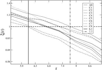
One may note that the amplitude of $\xi_{E}(r)$ varies in the different subsamples. Note that we refer to the amplitude variation of $\xi(r)$ as shown by Fig.11 without making a detailed analysis of the power-law exponent and the corresponding amplitude). The reason for this choice lies in the insignificant values of formal statistical errors along with large systematical errors (especially at large scales) due to the finite volume and single realization. Instead of performing precise estimation of $r_{0}$ and $\gamma$ we simply demonstrate the general behavior of $\xi$-function. This variation is due to fluctuations in the large scale distribution of galaxies and thus they are volume dependent effects. Therefore the amplitude of $\xi(r)$ is affected by finite-size effects as long as the distribution has not been found to have relaxed to an uniform system. From the one hand the Landy-Szalay estimator uses a sample density computed on the global sample scale, thus introducing a mixture of large scales and small scales properties in the measure of correlations. From the other hand, although the sample depth is of order of hundreds Mpc/h, finite size effects, related to the presence of large scale structures can be still important. The use of the conditional density avoids both these problems.

In order to explain the amplitude and slope variation observed by the estimation of two-properties by $\xi(r)$ we introduce a simple toy model which may capture the main element of the problem. However one may repeat the following argument for any distribution, and thus for any functional behavior of the conditional density, one finds in the data. The point is that in the regime of strong clustering, evidenced by the range of scales where $\Gamma(r)$ has not reached a clear flattening behavior, the determination of $\xi(r)$ and thus of the average density, is sample size dependent.

If the conditional density has a power-law behavior up to the size $r_{s}^{m}$ of the type

$$\Gamma(r)=Br^{-\gamma}$$ (21)

with $0<\gamma<3$ then the estimation of the sample average through the conditional density in spheres is

$$\Gamma^{*}(r_{s}^{m})=\frac{3}{4\pi(r_{s}^{m})^{3}}\int_{0}^{r_{s}^{m}}\Gamma(r)4\pi r^{2}dr=\frac{3B}{3-\gamma}(r_{s}^{m})^{-\gamma}\;.$$ (22)

Thus from Eq.19 we find that

$$\xi_{FS}(r)=\frac{3-\gamma}{3}\leavevmode\nobreak\ \left(\frac{r}{r_{s}^{m}}\right)^{-\gamma}-1\;.$$ (23)

One may note that Eq.23 easily takes into account both the amplitude variation in samples of different size, and the change of the slope as a function of scale (due to the different regime of strong correlation where the fit with a power-law is possible). From Eq.23 one may note that the slope depends on scale in a continuous way: for example at $r=r_{0}$ such that $\xi_{FS}(r_{0})=1$ one easily derives that the local slope becomes $2\gamma$ (see Fig.9). In fact, Hawkins et al. (2003) fitted the slope around the scale $r_{0}$ in the different samples (see their Tab.1) with the consistent result that the slope is $1.6$.

Moreover we would like to remark the crucial point that $\Gamma^{*}_{E}(r_{s}^{m})$ can differ from Eq.21 in a single sample determination: while the latter is the expectation value for the ensemble average quantity, the former quantity is subjected to large finite size fluctuations. This implies that the scaling of the amplitude of $\xi_{FS}(r)$ does not hold precisely in a single measurement, while this is the expectation in an ensemble of realizations (which is not possible to obtain in the analysis of a single sample).

5.2 The role of finite size effects in real space

Concerning the real space properties, we have not directly measured them here. However we may notice that the same finite-size effects which perturb the redshift space reduced two-point correlation function may affect the projected one (usually called $\omega(r_{p})$ — see e.g. Davis & Peebles 1983). In general, one may relate the real space $\xi_{RS}(R)$ to the projected $\omega(r_{p})$, where $r_{p}$ represents the projection of the redshift space distance on a direction perpendicular to the line of sight, through the following equation

$$\omega(r_{p})=2\int_{r_{p}}^{\infty}\frac{\xi_{RS}(y)y}{\sqrt{y^{2}-r_{p}^{2}}}dy\;.$$ (24)

Let us now consider the following situation: if the real space conditional density has the behavior $\Gamma_{RS}(R)=AR^{-\gamma}$ then we can repeat the argument which yields to Eq.23 with the result that

$$\xi_{RS}(R)=\frac{3-\gamma}{3}\left(\frac{R}{r_{s}^{m}}\right)^{-\gamma}-1$$ (25)

where $r_{s}^{m}$ is the sample depth, as discussed. Thus the real space $\xi_{RS}(R)$ shows the same finite-size effects present in the redshift space correlation function previously discussed. If $\xi_{RS}(R)$ has a pure power-law behavior with $\gamma>1$ then from Eq.24 one gets

$$\omega(r_{p})\sim r_{p}^{1-\gamma}\;.$$ (26)

In the present situation this is not the case, because the second term in Eq.25 gives an infinite contribution when integrated over all space. In practice however one truncates the integral to scales of order of $r_{s}^{m}$ and one expects to recover Eq.26 only at small enough scales. Thus

$$\omega(r_{p})=2\int_{r_{p}}^{r_{s}^{m}}\frac{\xi_{RS}(y)y}{\sqrt{y^{2}-r_{p}^{2}}}dy\;.$$ (27)

The finite size effect introduced by the cut-off $r_{s}^{m}$ may well take into account the observed shape of $\omega(r_{p})$. For example for $\gamma=0.8$ we get from Eq.25 and Eq.27 the behavior shown in Fig.12, which is very similar to the one measured by Hawkins et al. (2003). Hence, while in this example $\gamma<1$ we get that $\omega(r_{p})\sim r_{p}^{-1.5}$ in some finite range of scales: this is a finite size effect similar to the one varying the estimation of the exponent of the redshift space correlation function. Note that a similar finite-size effect may be present in the measurement of the angular two-point correlation function (see e.g., Montuori & Sylos Labini 1997).

Figure 12: Behavior of $\omega(r_{p})/r_{p}$ computed numerically from Eq.25 and Eq.27 with $\gamma=0.8$ and $r_{s}^{m}=70$ Mpc/h. The dashed line has a slope of $-1.5$.

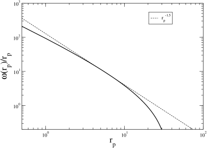
While we are clearly not able to make a definitive statement about whether the behavior of $\omega(r_{p})$ found by, for instance, Hawkins et al. (2003), is perturbed by systematic biases, our analysis shows that one needs to consider finite size effects explicitly also for the computation of the real space properties.

6 Discussion

We have studied redshift space correlation properties of six volume limited samples extracted from the 2dFGRS. We have considered several statistical properties. Particularly the characterization of small-scale properties through the nearest neighbor probability density allow us the determination of the smallest scale up to which correlations properties can be studied in a robust way. In fact, at scales smaller than the average distance between nearest neighbors, typically in the range of few Mpc/h (see Tab.2), discrete shot noise dominates the measurements leading to deviations from a power-law behavior. Whether the result of Zehavi et al. (2004), who found departures from a power law behavior in the galaxy correlation function of some samples of the SDSS catalog can be interpreted in this way, i.e. as dominated by nearest-neighbor correlations, is an open question, as they did not mention what is the average distance between nearest neighbors in their sample, and then they performed the analysis in real space instead of redshift space as we do here.

For the conditional average density we find that it is characterized fairly well by a power-law behavior in the range between 0.5 and 40 Mpc/h, where the exponent is $\gamma=0.8\pm 0.2$. This result is very robust at small scales ($r<$20 Mpc/h), as the volume average can be properly performed, and it becomes progressively weaker when the limits of the sample (set by the radius $r_{s}^{m}$ of the largest sphere fully contained in it) are reached. Systematic noise, due to un-averaged large fluctuations, increases when $r\rightarrow r_{s}^{m}$: one way to overcome this problem is to consider larger samples. In this respect it is useful to compare our results with the ones derived by Hogg et al. (2005) by analyzing the largest sample ever studied for this correlation analysis. In fact they considered a sample of luminous red galaxies, covering a volume of about $\sim 0.6$ (Gpc/h)³. They found the same power-law as we find here up to 20/30 Mpc/h. They then detected a slow crossover toward homogeneity which is eventually reached at 70 Mpc/h. With the data we have considered here, due to the limited solid angle of the survey, we are not able to confirm or disprove this result. In this respect it is worth noticing that, for example, Sylos Labini et al. (1998) found a similar value for the redshift space correlation exponent for the conditional density at those scales: extending the analysis to larger scales, with statistical tests of weaker robustness, they however found evidences for a continuation of correlations with almost the same exponent up to scales of order of one hundred Mpc/h. Apparently the results by Hogg et al. (2005) do not confirm such findings.

Leaving the question of the extension of the power-law behavior to further studies, we focus now on the interpretation of small-scale correlations. Up to the scale of few tens Mpc/h, the conditional density $\Gamma(r)$ show a power-law behavior, with exponent $\gamma=0.8\pm 0.2$ and well defined amplitude, although with some fluctuations in different sky regions. As discussed, the amplitude of the conditional density varies in different VL samples according to the luminosity of the galaxies selected. This has a very simple explanation, that brighter galaxies are less frequent than fainter ones. One can develop an analytical formalism by considering the effect of the galaxy luminosity function to understand this change: in the hypothesis that space and luminosity are not correlated, usually adopted in studies of large scale galaxy distribution, one can quantitatively compute the amplitude of the conditional density in different samples.

We have discussed that the results we get for the reduced two-point correlation function, although in agreement with the ones obtained by other groups, are affected by finite size effects. The reason is simply that as long as the distribution presents strong fluctuations, the study of $\xi(r)$ is problematic. The regime of strong fluctuations is described by a certain functional behavior of the conditional density $\Gamma(r)$, in the present case a power-law function. In this situation the estimation of the sample density is not only affected by large (statistical) noise, but it becomes sample size dependent, i.e. by a systematic effect. However because of the intrinsic large fluctuations systematic and statistical noise are entangled into the information provided by the amplitude of $\xi(r)$. Thus explicit tests for systematic finite size effects are needed, and these are provided by the analysis of the conditional density.

References

- (1) Baryshev, Yu., Teerikorpi P., 2005, Bull. Special Astrophys. Obs., 59 (in press) astro-ph/0505185
- (2) Basilakos, S., & Plionis, M., 2003 ApJ, 593, L91
- (3) Cole S. et al. (The 2dFGRS team) 2005 Mon.Not.R.Astr.Soc, in the press astro-ph/0501174
- (4) Colless M. et al. (The 2dFGRS team) 2003, astro-ph/0306581
- Davis & Peebles (1983) Davis, M. & Peebles, P.J.E., 1983, ApJ, 267, 46
- (6) Gabrielli A., Sylos Labini F., Joyce M., Pietronero L., 2004, Statistical physics for cosmic structures, (Springer Verlag)
- (7) Gaztanaga E., et al. (2005) astro-ph/0506249
- (8) Hawkins E., Maddox S., Cole S. et al. (The 2dFGRS team) 2003, MNRAS, 346, 78
- (9) Hogg D.W., Eisenstein D., Blanton M. et al., 2005, ApJ, 624, 54
- (10) Joyce M., Sylos Labini F., Gabrielli A., Montuori M., Pietronero L., 2005, A&A in press astro-ph/0501583
- (11) Joyce M., Montuori, M., Sylos Labini F., 1999, ApJ, 514, L5
- (12) Kerscher M., Szapudi I., Szalay A. S. 2000, ApJ, 535, L13
- (13) Landy S. D., Szalay A. 1993, ApJ, 412, 64
- (14) Madgwick D. S., Lahav O. et al. 2002, MNRAS, 333, 133
- (15) Madgwick et al. (The 2dFGRS team) 2003, MNRAS, 344, 847
- (16) Montuori, M. & Sylos Labini, F., 1997, ApJ, 487, L21
- (17) Norberg E., Baugh C., Hawkins E. et al. 2001, MNRAS, 328, 64
- (18) Norberg E., Baugh C., Hawkins E. et al. 2002, MNRAS, 332, 827
- (19) Peebles P. J. E., 1980, The Large-Scale Structure of the Universe (Princeton Univ. Press, Princeton, New Jersey)
- (20) Peebles, P.J.E., 2001 in “Historical Development of Modern Cosmology” ASP Conference Series Eds. V. J. Martinez, V. Trimble & M. J. Pons-Borderi, astro-ph/0103040
- (21) Peebles, P. J. E., 2001, ApJ, 557, 495
- (22) Sivakoff, G. R., Saslaw, W. C., 2005 ApJ, 626, 795
- (23) Sylos Labini F., Montuori M., Pietronero L. 1998 Phys. Rep., 293, 61
- (24) Sylos Labini F., 2005, astro-ph/0507277
- Tikhonov, Makarov & Kopylov (2000) Tikhonov, A.V., Makarov D.I, & Kopylov A.I., 2000, Bull.Spec.Astrophys.Obs., 50, 39
- Tikhonov & Makarov (2003) Tikhonov, A. V.; Makarov, D. I., 2003, Astronomy Lett., 29, 289
- York et al. (2000) York, D., et al., 2000, AJ, 120, 1579
- Zehavi et al. (2004) Zehavi et al., 2004 ApJ, 608, 16