On the relation between Hot-Jupiters and the Roche Limit

Abstract

Many of the known extrasolar planets are “hot Jupiters,” giant planets with orbital periods of just a few days. We use the observed distribution of hot Jupiters to constrain the location of the “inner edge” and planet migration theory. If we assume the location of the inner edge is proportional to the Roche limit, then we find that this edge is located near twice the Roche limit, as expected if the planets were circularized from a highly eccentric orbit. If confirmed, this result would place significant limits on migration via slow inspiral. However, if we relax our assumption for the slope of the inner edge, then the current sample of hot Jupiters is not sufficient to provide a precise constraint on both the location and power law index of the inner edge.

¹Astronomy Department, UC Berkeley, 601 Campbell Hall, Berkeley, CA 94709, USA [eford@astro.berkeley.edu]

²Dept. of Physics & Astronomy, Northwestern, 2145 Sheridan Road, Evanston, IL 60208-834 [rasio@northwestern.edu]

1. Introduction

Early radial velocity discoveries were interpreted as showing a pile-up at an orbital period of three days, but recent transit surveys and very sensitive radial velocity observations have discovered planets with even shorter orbital periods. These discoveries suggest that the inner edge for hot Jupiters is not defined by an orbital period, but rather by a tidal limit which depends on both the semi-major axis and the planet-star mass ratio (See Fig. 1). This would arise naturally if the inner edge were related to the Roche limit, the critical distance at which a planet fills its Roche lobe. The Roche limit, $a_{R}$ is is defined by

$$R_{P}=0.462a_{R}\left(\frac{M_{P}}{M_{*}}\right)^{1/3}$$ (1)

where $R_{P}$ is the radius of the planet, $M_{P}$ is the mass of the planet, and $M_{*}$ is the mass of the star.

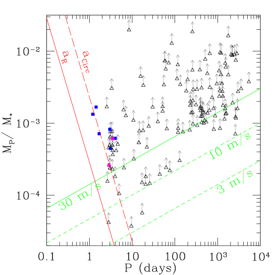
Figure 1.: Minimum mass ratio versus orbital period for the current observed sample of planetary companions. Planets discovered by radial velocity surveys are shown as triangles with arrows indicating $1-\sigma$ uncertainties in mass due to unknown inclination. The magenta squares have inclinations and radii measured via transits. The blue squares show planets discovered by transit searches. The green lines show the minimum mass corresponding to various velocity semi-amplitudes and roughly indicate where radial velocity surveys are nearly complete ($\geq 30$m/s), have significant sensitivity ($\geq 10$m/s), and are only beginning to detect planets ($\geq 3$m/s). The two red lines show the the location of the Roche limit ($a_{R}$) and the ideal circularization radius ($a_{\rm circ}$) for a planet with a radius, $R_{P}=1.2R_{J}$. The inner edge for the distribution of hot Jupiters is near $a_{\rm circ}$. Note that the red lines do not apply to the lowest mass planets that likely have a radius significantly less than $1.2R_{J}$ due to their qualitatively different internal structure.

The numerous mechanisms proposed to explain the migration of giant planets to short period orbits can be divided into two broad categories:

1. Mechanisms involving slow inspiral, such as migration due to a gaseous disk or planetesimal scattering (Trilling et al. 1998, Gu et al. 2003). These would result in a limiting separation equal to the Roche limit.

2. Mechanisms involving the circularization of highly eccentric orbits with small pericenter distances, possibility due to planet-planet scattering (Rasio & Ford 1996, Ford, Havlickova, & Rasio 2001, Papaloizou & Terquem 2001, Marzari & Weidenschilling 2002), secular perturbations from a wide binary companion (Holman, Touma & Tremaine 1997), or tidal-capture of free-floating planets (Gaudi 2003). These would result in a limiting separation of twice the Roche limit (Faber et al. 2004).

2. Statistical Analysis

To quantitatively explore the observational constraints on the distribution of hot Jupiters, we employ the techniques of Bayesian inference. In the Bayesian framework, the model parameters are treated as random variables which can be constrained by the actual observations. Therefore, to perform a Bayesian analysis it is necessary to specify both the likelihood (the probability of making a certain observation given a particular set of model parameters) and the the prior (the a priori probability distribution for the model parameters). Let us denote the model parameters by $\theta$ and the actual observational data by $d$, so that the joint probability distribution for the observational data and the model parameters is given by

$$p(d,\theta)=p(\theta)p(d|\theta)=p(d)p(\theta|d),$$ (2)

where we have expanded the joint probability distribution in two ways and both are expressed as the product of a marginalized probability distribution and a conditional probability distribution. The prior is given by $p(\theta)$ and the likelihood by $p(d|\theta)$. On the far right hand side, $p(d)$ is the a priori probability for observing the values actually measured and $p(\theta|d)$ is the probability distribution of primary interest, the a posteriori probability distribution for the model parameters conditioned on the actual observations, or simply the posterior. The probability of the observations $p(d)$ can be obtained by marginalizing over the joint probability density and again expanding the joint density as the product of the prior and the likelihood. This leads to Bayes’ theorem, the primary tool for Bayesian inference,

$$p(\theta|d)=\frac{p(d|\theta)p(\theta)}{p(d)}=\frac{p(d|\theta)p(\theta)}{\int\,d\theta p(d|\theta)p(\theta)}$$ (3)

Often the model parameters contain one or more parameters of particular interest (e.g., the location of the inner cutoff for hot Jupiters in our analysis) and other nuisance parameters which are necessary to adequately describe the observations (e.g., the fraction of stars with hot Jupiters in our analysis). Since Bayes’ theorem provides a real probability distribution for the model parameters, we can simply marginalize over the nuisance parameters to calculate a marginalized posterior probability density, which will be the basis for making inferences about the location of the inner cutoff for hot Jupiters.

We construct models for the distribution of hot Jupiters and use Bayes’ theorem to calculate posterior probability distributions for model parameters given the orbital parameters measured for extrasolar planets discovered by radial velocity surveys. For the sake of clarity, we start by presenting a simplistic one-dimensional model for the distribution of hot Jupiters. We then gradually improve our model to understand how each model improvement affects our results.

The primary question which we wish to address in this paper is the location of the inner edge of the distribution of hot Jupiters relative to the location of the Roche limit. Therefore, we define $x\equiv a/a_{R}$, where $a$ is the semi-major axis of the planet and $a_{R}$ is the Roche limit. We assume that the actual distribution of $x$ for various hot Jupiters is given by a truncated power law,

$$p(x|\gamma,x_{l},x_{u})dx=x^{\gamma}\left(\frac{dx}{x}\right),\quad x_{l}<x<x_{u},$$ (4)

and zero else where. Here $\gamma$ is the power law index and $x_{l}$ and $x_{u}$ are the lower and upper limits for $x$. The lower limit, $x_{l}$, is the model parameter of primary interest, while $\gamma$ and $x_{u}$ are nuisance parameters. Therefore, our results are summarized by the marginalized posterior probability distribution for $x_{l}$.

In order to minimize complexities related to the analysis of a population, we choose to restrict our analysis to a subset of the known extrasolar planets for which radial velocity surveys are complete and extremely unlikely to contain any false positives. To obtain such a sample, we impose two constraints: $P\leq P_{\max}$, where $P_{\max}$ is the maximum orbital period, and $K\geq K_{\min}$, where $K_{\min}$ is the minimum velocity semi-amplitude. We use $K_{\min}=30$m/s, based on the results of simulated radial velocity surveys (Cumming 2004). We typically set $P_{\max}=$30d, even though radial velocity surveys are likely to be complete even for longer orbital periods (provided $K\geq K_{\min}$). This minimizes the chance of introducing biases due to survey incompleteness or possible structure in the observed distribution of planet orbital periods at larger periods. By considering only planets with orbital parameters such that radial velocity surveys are very nearly complete, our analysis does not depend on the velocities of stars for which no planets have been discovered. Note that our criteria for including a planet may introduce a bias depending on the actual mass-period distribution. We will address this point with a two-dimensional model at the end of our analysis. Also, our criteria exclude any planet discovered via techniques other than radial velocities (e.g., transits), even if subsequent radial velocity observations were obtained to confirm the planet.

Initially, we make several simplifying assumptions to make an analytic treatment possible. We assume uniform prior probability distributions for each of the model parameters, $p(\gamma)\sim U(\gamma_{\min},\gamma_{\max})$ and $p(x_{l},x_{u})\sim\mathrm{const}$, provided $x_{ll}<x_{l}<x_{u}<x_{uu}$ and zero otherwise. The lower and upper limits ($x_{ll}$ and $x_{uu}$) for each parameter are chosen to be sufficiently far removed from regions of high likelihood that the limits do not affect the results. We assume that the orbital period ($P$), velocity semi-amplitude ($K$), semi-major axis ($a$), stellar mass ($M_{*}$), and planet mass times the sin of the inclination of the orbit relative to the line of sight ($m\sin i$) are known exactly based on the observations.

We begin by assuming that $\sin i=1$ for all planets and that all planets have the same radius, $R_{P}$. With these assumptions, the posterior probability distribution is given by

$$p(x_{l},x_{u},\gamma|x_{1},...x_{n})\sim\gamma^{n}(x_{u}^{\gamma}-x_{l}^{\gamma})^{-n}\prod_{j=1}^{n}x_{j}^{\gamma-1},$$ (5)

provided that $x_{ll}<x_{l}\leq x_{(1)}\leq x_{(n)}\leq x_{u}<x_{uu}$ and $\gamma_{\min}<\gamma<\gamma_{\max}$. Here $n$ is the number of planets included in the analysis, $x_{(1)}$ is the smallest value of $x$ among the sample of hot Jupiters used in the analysis, and $x_{(n)}$ is the largest value of $x$ in the sample. The normalization can be obtained by integrating over all allowed values of $x_{l}$, $x_{u}$, and $\gamma$.

We show the marginal posterior distributions in which we have integrated over the nuisance parameters, $x_{u}$ and $\gamma$ in Fig. 2 (left, dotted line), assuming $R_{P}=1.2R_{J}$. The distribution has a sharp cutoff at $x_{(1)}$ and a tail to lower values reflecting the chance that $x_{l}<x_{(1)}$ due to the finite sample size.

Figure 2.: Left: Marginal posterior distribution for $x_{l}$, the location of the inner edge for the population of hot Jupiters. The dotted line assumes all systems are viewed edge on ($\sin i=1$). The solid line assumes an isotropic distribution of orbital inclinations (except for transiting planets). The remaining lines replace the assumption of $R=1.2R_{J}$ for all non-transiting planets with a normal distribution for the planet radii using a dispersion dispersion of $\sigma_{R_{P}}=0.05R_{J}$ (long dashes), $0.1R_{J}$ (dots-dashes), or $0.2R_{J}$ (short dashes). Upper Right: Dependence of the marginal posterior distribution for $x_{l}$ on the assumed mean planet radius. $\left<R_{P}\right>=1.0R_{J}$ (long dashes), $1.1R_{J}$ (dotted), $1.2R_{J}$ (solid), $1.3R_{J}$ (dotted dashed), and $1.4R_{J}$ (short dashes), all assuming $\sigma_{R_{P}}=0.1R_{J}$. Lower Right: Same as above, but using a 2-d model (period & mass) which accounts for selection effects.

Next, we assume that the actual distribution of orbital inclinations is isotropic ($\cos i\sim U[-1,1]$). For planets which were discovered by radial velocities and the inclination was subsequently determined with the detection of transits, we use the measured inclination. The marginal posterior distribution for $x_{l}$ is shown in Fig. 2 (left, solid line). The sharp cutoff at $x_{(1)}$ is replaced with a more gradual tail, reflecting the chance that $\sin i<1$ for planets with the smallest values of $x$.

Next, we consider the consequences of allowing for a distribution of planetary radii. For transiting planets we use a normal distribution for the radius based on the published radius and uncertainty. For nontransitting planets, we assume a normal distribution of planetary radii with standard deviation, $\sigma_{R_{P}}$. We show the resulting marginalized posterior distributions in Fig. 2 (left). Allowing for a significant dispersion broadens the posterior distribution for $x_{l}$ and results in a slight shift to smaller values.

We have also explored the effects of varying the model parameter $P_{\max}$, exploring values from 8d to 60d. We find that this does not make a discernible difference in the posterior distribution for $x_{l}$.

Our results are sensitive to our choice for the mean radius for the non-transiting planets. In Fig. 2 (upper right) we show the posterior distributions for various mean radii, assuming $\sigma_{R_{P}}=0.1R_{J}$. Since few planets have a known inclination, there is be a nearly perfect degeneracy between $R_{P}$ and $x_{l}$. Even when we include transiting planets, this degeneracy remains near perfect, i.e., $p(x_{l}|R_{p},x_{1},...,x_{n})\simeq p(x_{l}\cdot\frac{R^{\prime}_{P}}{R_{P}}|R^{\prime}_{P},x_{1},...,x_{n})$. However, it can be seen that is extremely unlikely for $x_{l}$ to be near unity for any reasonable planetary radius.

We have also performed an improved analysis using a two dimensional model which considers the joint planet mass-period distribution function. This allows us to account for observational selection biases due to the minimum mass for detecting a planet depending on the orbital period. We assume that the distribution function is a truncated power law in both planet-star mass ratio and period. That is

$$p(P,\mu|\alpha,\beta,P_{\min}P_{\max},\mu_{\min},\mu_{\max},c)\sim cP^{\alpha}\mu^{\beta}\frac{dP}{P}\frac{d\mu}{mu},$$ (6)

provided $\mu_{\min}<\mu<\mu_{\max}$, $P<P_{\max}$, and $a(P,M_{*})\geq x_{l}\cdot a_{R}(R_{P},\mu)$. Here $\mu=M_{P}/M_{*}$, and $\alpha$ and $\beta$ are the new power law indices. We find the marginal posterior distribution for $x_{l}$ is very similar to the results of our 1-d analysis. The most significant difference is that the posterior distribution for $x_{l}$ shifts slightly to wards larger separations (see Fig. 2, lower right).

3. Discussion

The current distribution of hot Jupiters discovered by radial velocity searches shows a cutoff that is a function of orbital period and planet mass. Our Bayesian analysis solidly rejects the hypothesis that the cutoff occurs inside or at the Roche limit, in contrast to what would be expected if the hot Jupiters had slowly migrated inwards on a circular orbit. Instead, our analysis shows that this cutoff occurs at a distance nearly twice that of the Roche limit, as expected if the hot Jupiters were circularized from a highly eccentric orbit. These findings suggest that hot Jupiters may have formed via planet-planet scattering (e.g., Rasio & Ford 1996), tidal capture of free floating planets (Gaudi 2003), or secular perturbations from a highly inclined binary companion (e.g., Holman, Touma & Tremaine 1997). If the hot Jupiters indeed were circularized from a high eccentricity orbit, then this raises the challenge of explaining the origin of giant planets with orbital periods $\sim 10-100$ days.

An alternative explanation is that the planets migrated inwards on a nearly circular orbit at a time when the planets were roughly twice their current radii. Future observations of low mass planets may make it possible to test this alternative, assuming that the time evolution of their contraction is significantly different than for Jupiter-mass planets. A third alternative is that short-period giant planets are destroyed by another process before they reach the Roche limit. HST observations of HD 209458 indicate absorption by matter presently beyond the Roche lobe of the planet and have been interpreted as evidence for a wind leaving the planet powered by stellar radiation (Vidal-Madjar et al. 2003, 2004). Further theoretical work will help determine under what conditions these processes can cause significant mass loss.

Future planet discoveries will either tighten the constraints on the model parameters or provide evidence for the existence of planets definitely closer than twice the Roche limit. In particular, new discoveries of very low mass planets could better constrain the shape of the inner cutoff as a function of mass. In the future, an improved analysis could also include such low-mass planets where surveys are not yet complete. For future theoretical work, we hope to explore the possibility of orbital circularization occurring at larger orbital radii, possibly in a protoplanetary disk or while the star is young and still contracting.

• We thank Eugene Chiang, Tom Loredo, Norm Murray, Ruth Murray-Clay, John Papaloizou, Frederic Pont for their comments. This research was supported by NSF grants AST-0206182 and AST0507727 at Northwester and a Miller Research Fellowship at UC Berkeley.

References

Cumming, A. 2004, MNRAS, 354, 1165.

Faber, J.A., Rasio, F.A. & Willems, B. 2005, Icarus, 175, 248.

Ford, E.B., Havlickova, M., & Rasio, F.A. 2001, Icarus, 150, 303.

Gaudi, S. 2003, astro-ph/0307280.

Gu, P.-G., Lin, D.N.C. & Bodenheimer P.H. 2003, ApJ, 558, 509.

Holman, M., Touma, T. & Tremaine, S. 1997, Nature, 386, 254.

Marzari, F. & Weidenschilling, S.J. 2002, Icarus 156, 670.

Papaloizou, J.C.B. & Terquem, C. 2001, MNRAS, 325, 221.

Rasio, F.A. & Ford, E.B. 1996, Science, 274, 954.

Trilling, D. E., Benz, W., Guillot, T., Lunine, J. I., Hubbard, W. B., & Burrows, A. 1998, ApJ, 500, 428.

Vidal-Madjar, A., Lecavelier des Etangs, A., Desert, J.-M., Ballester, G.E., Ferlet, R., Hebrand, G., Mayor, M. 2003, Nature, 422, 143.

Vidal-Madjar, A., Desert, J.-M., Lecavelier des Etangs, A., Hibrard, G., Ballester, G. E., Ehrenreich, D., Ferlet, R., McConnell, J. C., Mayor, M., & Parkinson, 2004, ApJL 604, 69.