Reconciling the ultra-high energy cosmic ray spectrum with Fermi shock acceleration

Abstract

The energy spectrum of ultra-high energy cosmic rays (UHECR) is usually calculated for sources with identical properties. Assuming that all sources can accelerate UHECR protons to the same extremely high maximal energy $E_{\max}>10^{20}$ eV and have the steeply falling injection spectrum $1/E^{2.7}$, one can reproduce the measured cosmic ray flux above $E\raise 1.29167pt\hbox{$\;>$\kern-7.5pt\raise-4.73611pt\hbox{$\sim\;$}}10^{18}$ eV. We show that relaxing the assumption of identical sources and using a power-law distribution of their maximal energy allows one to explain the observed UHECR spectrum with the injection $1/E^{2}$ predicted by Fermi shock acceleration.

PACS: 98.70.Sa

1 Introduction

The origin and the composition of ultra-high energy cosmic rays (UHECR) are still unknown. Chemical composition studies [1, 2] of the CR flux of both the AGASA [3] and HiRes [4] experiments point to the dominance of protons above $10^{18}$ eV, but depend strongly on the details of hadronic interaction models used. Another signature for extragalactic protons is a dip in the CR flux around $5\times 10^{18}$ eV seen in the experimental data of AGASA, Fly’s Eye, HiRes and Yakutsk. This dip may be caused by energy losses of protons due to $e^{+}e^{-}$ pair production on cosmic microwave photons [5, 6] and was interpreted first by the authors of Ref. [7] as signature for the dominance of extragalactic protons in the CR flux. Finally, the UHECR proton spectrum should be strongly suppressed above $E\raise 1.29167pt\hbox{$\;>$\kern-7.5pt\raise-4.73611pt\hbox{$\sim\;$}}5\times 10^{19}$ eV due to pion production on cosmic microwave photons, the so called Greisen-Zatsepin-Kuzmin (GZK) cutoff [8]. The evidence for or against the presence of this cutoff in the experimental data is at present contradictory.

In this work, we assume following Ref. [7] that UHECRs with $E\raise 1.29167pt\hbox{$\;>$\kern-7.5pt\raise-4.73611pt\hbox{$\sim\;$}}10^{18}$ eV are mostly extragalactic protons and compare the theoretical predictions for their energy spectrum to experimental data. Several groups of authors have tried previously to explain the observed spectral shape of UHECR flux using mainly two different approaches: In the first one, the ankle is identified with the transition from a steep galactic, usually iron-dominated component to extragalactic protons with injection spectrum between $\sim 1/E^{2}$ and $1/E^{2.2}$ [9, 10, 11, 12, 13, 14]. In the second approach, the dip is a feature of $e^{+}e^{-}$ pair production and one is able to fit the UHECR spectrum down to $E\sim 10^{18}$ eV using only extragalactic protons and an injection spectrum between $1/E^{2.6}$ and $1/E^{2.7}$ [7, 15, 16, 17]. The first possibility is not very predictive and probably in contradiction to the observed isotropy of the UHECR flux [18], while for the second one an explanation for the complex spectrum suggested ad-hoc by the authors of Ref. [7] is missing. Moreover, an injection spectrum $1/E^{\alpha}$ with $\alpha\approx 2.7$ is considerably steeper than $\alpha\approx 2$ predicted by shock acceleration [19].

A basic ingredient of all these analyses is the assumption that the sources are identical. In particular, it is assumed that every source can accelerate protons to the same maximal energy $E_{\max}$, typically chosen as $10^{21}$ eV or higher. However, one expects that $E_{\max}$ differs among the sources and that the number of potential sources becomes smaller and smaller for larger $E_{\max}$. Therefore two natural questions to ask are i) can one explain the observed CR spectrum with non-identical sources? And ii), is in this case a good fit of the CR spectrum possible with $\alpha\sim 2$ as predicted by Fermi shock acceleration?

In this letter, we address these two questions and show that choosing a power-law distribution $dn/dE_{\max}\propto E_{\max}^{-\beta}$ for $E_{\max}$ allows one to explain the measured energy spectrum e.g. for $\alpha=2$ with $\beta=1.7$.

2 Fitting the AGASA and HIRES data

We assume a continuous distribution of CR sources with constant comoving density up to the maximal redshift $z_{\max}=2$. The flux of sources further away is negligible above $10^{18}$ eV, the lowest energy considered by us. For simplicity, we assume the same luminosity for all sources. Then UHECRs are generated according to the injection spectrum

$$\frac{dN}{dE}\propto E^{-\alpha}\,\vartheta(E_{\max}-E)\,,$$ (1)

and are propagated until their energy is below $10^{18}$ eV or they reach the Earth. The proton propagation was simulated with the Monte Carlo code of Ref. [20]. The maximal energy $E_{\max}$ in Eq. (1) is usually chosen as $E_{\max}=10^{21}$ eV or larger for identical sources. In this case, the exact value of $E_{\max}$ influences only the UHECR flux above $\sim 5\times 10^{19}$ eV, i.e. the strength of the GZK suppression, while the flux at lower energies is independent from $E_{\max}$.

The shape of the observed energy spectrum between $E\approx 10^{18}$ eV and the GZK cutoff can be well explained by the modification of the power-law injection spectrum through the energy losses of extragalactic protons due to pion and $e^{+}e^{-}$ pair production on cosmic microwave photons [6, 7]. In particular, one can reproduce both the HiRes data [4] and the Akeno/AGASA data (below $10^{20}$ eV) with $\alpha=2.7$, cf. Figs. 1, 2 and Refs. [7, 15]. In order to combine the AGASA [3] with the Akeno [21] data in Fig. 2, we have rescaled systematically the AGASA data 10% downwards in energy which is well within the uncertainty of the absolute energy scale of AGASA [3].

The use of a power-law for the injection spectrum of UHECRs is well-motivated by models of shock acceleration [19]. However, these models predict as exponent typically $\alpha\approx 2.0$–2.2. Moreover, the maximal acceleration energy of a certain source depends obviously on parameters that vary from source to source like its magnetic field strength or its size [22, 23]. Therefore, one expects that $E_{\max}$ varies vastly among different sources with less and less sources able to accelerate cosmic rays to the high-energy end of the spectrum.

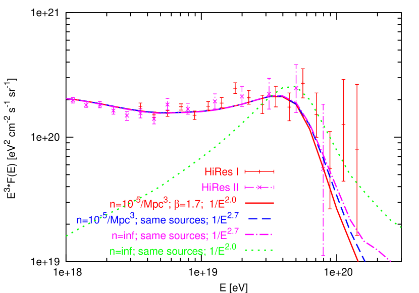
Figure 1: Fits of the HiRes I and HiRes II data are shown for a uniform distribution of identical sources with power-law injection spectrum $1/E^{2}$ (green, dashed line) and $1/E^{2.7}$ (magenta, dash-dotted line) for an infinite number of sources as well as for a realistic source density $n_{s}=10^{-5}/{\rm Mpc}^{3}$ and spectrum $1/E^{2.7}$ (blue, dashed line). The case of an $1/E^{2}$ spectrum and maximal energy dependence from Eq. (2) with $\beta=1.7$ is shown as a red, solid line.

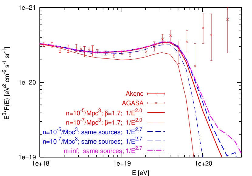
Figure 2: The fit of Akeno/AGASA data using a uniform distribution of identical sources for an infinite number of sources and power-law spectrum $1/E^{2.7}$ is shown as a magenta, dash-dotted line. The same fit with the realistic source density $n_{s}=10^{-5}/{\rm Mpc}^{3}$ and spectrum $1/E^{2.7}$ (thick blue dashed line) and $1/E^{2}$ spectrum and maximal energy dependence from Eq. (2) with $\beta=1.7$ is shown as a thick red, solid line. The thin red, solid line for the spectrum $1/E^{2}$ and $\beta=1.7$ and the thin blue, dashed line for the spectrum $1/E^{2.7}$ correspond to the low source density $n_{s}=10^{-7}/{\rm Mpc}^{3}$.

Here, we propose to use more realistic source models for the calculation of the energy spectrum expected from extragalactic protons. We relax the assumption of identical sources and suggest to use a power-law distribution for the maximal energies of the individual sources,

$$\frac{dn}{dE_{\max}}\propto E_{\max}^{-\beta}\,.$$ (2)

Without concrete models for the sources of UHECRs, we cannot derive the exact form of the distribution of $E_{\max}$ values. However, the use of a power-law for the $E_{\max}$ distribution is strongly motivated by the following two reasons: First, we expect a monotonically decreasing distribution of $E_{\max}$ values and, for the limited range of two energy decades we consider, a power-law distribution should be a good approximation to reality. Second, the use of a power-law distribution for $E_{\max}$ with exponent

$$\beta=\alpha+1-\alpha_{0}\,,$$ (3)

guaranties to recover the spectra calculated with Eq. (1), i.e. $E_{\max}=$ const., for the special case of $E_{\max}\to\infty$ and a continous distribution of sources. In Eq. (3), $\alpha$ denotes the exponent of the injection spectrum of an individual source and $\alpha_{0}$ the exponent of the effective injection spectrum after averaging over the $E_{\max}$ distribution of individual sources. For instance, an injection spectrum of single sources with $\alpha=2$ characteristic for Fermi shock acceleration reproduces effectively together with a distribution of $E_{\max}$ values with $\beta=1.7$ the case $\alpha_{0}=2.7$ found assuming identical sources. For finite values of $E_{\max}$ and the source density $n_{s}$, the effective injection spectrum is not described anymore by a single power-law. However, deviations show-up only at energies above $\approx 6\times 10^{19}$ eV or small source densities, see below.

The results for 5.000 Monte Carlo runs of our simulation are presented in Fig. 1 for HiRes and in Fig. 2 for Akeno/AGASA. In the standard picture of uniform sources with identical maximal energy (here, $E_{\max}=10^{21}$ eV) and $1/E^{2}$ spectrum, extragalactic sources contribute only to a few bins of the spectrum around the GZK cutoff, cf. the green-dotted line in Fig. 1. By contrast, an injection spectrum $1/E^{2.7}$ allows one to explains the observed data down to $\approx 10^{18}$ eV with extragalactic protons from identical sources, cf. the magenta, dash-dotted line for a continuous and the blue, dashed line for a finite source distribution with $n_{s}=10^{-5}/{\rm Mpc}^{3}$ in Fig. 1. This well-known result can be obtained also for an injection spectrum $1/E^{2}$ of individual sources, if for the $E_{\max}$ distribution, Eq. (2), the exponent $\beta=1.7$ is chosen. This is illustrated by the red, solid line in Fig. 1 for the case of a finite source density $n_{s}=10^{-5}/{\rm Mpc}^{3}$. As already announced, only small differences at the highest energies, $E\raise 1.29167pt\hbox{$\;>$\kern-7.5pt\raise-4.73611pt\hbox{$\sim\;$}}6\times 10^{19}$ eV, are visible between an effective $\alpha_{0}=2.7$ produced by an suitable $E_{\max}$ distribution and the case of identical sources with $\alpha=2.7$ for large enough $n_{s}$.

In Fig. 2, we show the dependence of our results on the source density $n_{s}$ together with the Akeno/AGASA data. While for large enough source densities, $n_{s}=10^{-5}/{\rm Mpc}^{3}$, the spectra from identical sources with $1/E^{2.7}$ and from sources with $1/E^{2}$ injection spectrum, variable $E_{\max}$ and $\beta=1.7$ are very similar, for smaller densities, $n=10^{-7}/{\rm Mpc}^{3}$ in Fig. 2, the shape of the spectra differs considerably even at lower energies. Thus for small source densities, the best-fit parameter for $\alpha$ and the quality of the fit has to be determined for each combination of $\beta$ and $n_{s}$ separately and the relation (3) is not valid anymore.

From our results presented in Figs. 1 and  2, we conclude that the power-law injection spectrum $1/E^{2.7}$ found earlier may be seen as a the combined effect of an injection spectrum $1/E^{2}$ predicted by Fermi acceleration and a power-law distribution of the maximal energies of individual sources with $\beta=1.7$, if the source density is sufficiently large, $n_{s}\raise 1.29167pt\hbox{$\;>$\kern-7.5pt\raise-4.73611pt\hbox{$\sim\;$}}10^{-5}/{\rm Mpc}^{3}$. More generally, the exponent $\alpha_{0}$ obtained from fits assuming identical sources is connected simply by Eq. (3) to the parameters $\alpha$ and $\beta$ determining the power-laws of variable sources in this regime.

3 Discussion

The minimal model we proposed can explain the observed UHECR spectrum for $E>10^{18}$ eV with an injection spectrum as predicted by Fermi acceleration mechanism, $\alpha=2$–2.2. However, in general the experimental data can be fitted for any value of $\alpha$ in the range $2\leq\alpha\leq 2.7$ by choosing an appropriate index $\beta=\alpha+1-\alpha_{0}$ in Eq. (2). The best-fit injection spectrum with $\alpha=2.7$ found for $E_{\max}=$ const. appears in our model as an effective value that takes into account the averaging over the distribution of $E_{\max}$ values for various sources.

As in the standard case of identical sources, we can not explain the AGASA excess at $E>10^{20}$ eV in our model. Both injection spectra $1/E^{2.7}$ and $1/E^{2}$ do not fit well the last three AGASA bins above $10^{20}$ eV; they have $\chi^{2}=9.8$ and $\chi^{2}=7.9$ respectively. The shape of the dip can be used also in our model to understand the overall energy scale of different experiments as suggested in Ref. [7, 24].

For completeness, we consider now the case of sources with variable luminosity. The total source luminosity can be defined by

$$L(z)=L_{0}(1+z)^{m}\vartheta(z_{\max}-z)\vartheta(z-z_{\min})\,,$$ (4)

where $m$ parameterizes the luminosity evolution, and $z_{\min}$ and $z_{\max}$ are the redshifts of the closest and most distant sources. Sources in the range $2<z<z_{\max}$ have a negligible contribution to the UHECR flux above $10^{18}$ eV. The value of $z_{\min}$ is connected to the density of sources and influences strongly the shape of bump and the strength of the GZK suppression [20, 25].

The value of $m$ influences the spectrum in the range $10^{18}~{}{\rm eV}<E<10^{19}$ eV [7], but less strongly than the parameter $\beta$ from Eq. (2). Positive values of $m$ increase the contribution of high-redshift sources and, as a result, injection spectra with $\alpha<2.7$ can fit the observed data even in the case of the same $E_{\max}$ for all sources. For example, $\alpha=2.6$ and $m=3$ fits the AGASA and HiRes data as well as $\alpha=2.7$ and $m=0$ ($\chi^{2}/{\rm d.o.f.}<1$). However, a good fit with $\alpha=2$ requires a unrealistic strong redshift evolution of the sources, $m=16$.

We have presented fits of our model only to the data of Akeno/AGASA and HiRes. Similar fits can be done for the first results of the Pierre Auger Observatory [26] or the older data of the Yakutsk experiment [27]. However, the systematic uncertainty of these data sets is (still) too large, and at present no further insight can be gained from these data. In the future, data of the Pierre Auger Observatory [26] and the Telescope Array [28] will restrict the parameter space of theoretical models similar to one presented here. If a clustered component or even individual sources can be identified in the future data, their spectra will allow one to distinguish between different possibilities for the injection spectrum. Intriguingly, the energy spectrum of the clustered component found by the AGASA experiment is much steeper than the overall spectrum [29]. Thus, one might speculate this steeper spectrum is the first evidence for the ”true” injection spectrum of UHECR sources.

4 Summary

In this Letter we have argued that the assumption that all UHECR sources accelerate to the same maximal energy is both unrealistic and unnecessary. Abandoning the idea of identical sources and introducing a power-law distribution for the maximal energy of UHECR sources allows one to fit the CR spectrum above $10^{18}$ eV with the canonical $1/E^{2}$ spectrum predicted by Fermi acceleration introducing $\beta$ as one additional, physically well-motivated parameter. The exponent $\alpha=2.7$ of the best-fit injection spectrum for identical sources appears in or model only as an effective parameter, determined by the exponents from the “true” injection spectrum and from the distribution of $E_{\max}$ values.

References

- [1] K. Shinozaki et al., Proc. 28th ICRC (Tsukuba), 1, 437 (2003).
- [2] D. R. Bergman et al., Proc. 29th ICRC (Pune), 2005 [astro-ph/0507483.
- [3] M. Takeda et al., Astropart. Phys. 19, 447 (2003) [astro-ph/0209422].
- [4] R. U. Abbasi et al., Phys. Rev. Lett. 92, 151101 (2004) [astro-ph/0208243]; D. R. Bergman [the HiRes Collaboration], astro-ph/0507484.
- [5] C. T. Hill and D. N. Schramm, Phys. Rev. D 31, 564 (1985).
- [6] V. S. Berezinsky and S. I. Grigor’eva, Astron. Astrophys. 199, 1 (1988).
- [7] V. Berezinsky, A. Z. Gazizov and S. I. Grigorieva, hep-ph/0204357; astro-ph/0210095; Nucl. Phys. Proc. Suppl. 136, 147 (2004) [astro-ph/0410650]; Phys. Lett. B 612 (2005) 147 [astro-ph/0502550].
- [8] K. Greisen, Phys. Rev. Lett. 16, 748 (1966); G. T. Zatsepin and V. A. Kuzmin, JETP Lett. 4, 78 (1966) [Pisma Zh. Eksp. Teor. Fiz. 4, 114 (1966)].
- [9] C. T. Hill, D. N. Schramm and T. P. Walker, Phys. Rev. D 34, 1622 (1986).
- [10] J. P. Rachen, T. Stanev and P. L. Biermann, Astron. Astrophys. 273, 377 (1993) [astro-ph/9302005].
- [11] J. N. Bahcall and E. Waxman, Phys. Lett. B 556, 1 (2003) [hep-ph/0206217].
- [12] T. Wibig and A. W. Wolfendale, J. Phys. G 31, 255 (2005) [astro-ph/0410624].
- [13] D. Allard, E. Parizot, E. Khan, S. Goriely and A. V. Olinto, astro-ph/0505566.
- [14] D. De Marco and T. Stanev, astro-ph/0506318.
- [15] D. De Marco, P. Blasi and A. V. Olinto, Astropart. Phys. 20, 53 (2003) [astro-ph/0301497].
- [16] M. Lemoine, Phys. Rev. D 71, 083007 (2005) [astro-ph/0411173].
- [17] F. W. Stecker and S. T. Scully, Astropart. Phys. 23, 203 (2005) [astro-ph/0412495].
- [18] M. Kachelrieß, P. D. Serpico and M. Teshima, astro-ph/0510444.
- [19] V. S. Berezinskii et al, Astrophysics of cosmic rays, Amsterdam: North-Holland 1990. T. Gaisser, Cosmic Rays and Particle Physics, Cambridge University Press 1991.
- [20] M. Kachelrieß and D. Semikoz, Astropart. Phys. 23, 486 (2005) [astro-ph/0405258].
- [21] M. Nagano et al., J. Phys. G10, 1295 (1984).
- [22] R. J. Protheroe and R. W. Clay, Publ. Astron. Soc. of Australia 21, 1 (2004) [astro-ph/0311466].
- [23] R. J. Protheroe, Astropart. Phys. 21, 415 (2004) [astro-ph/0401523].
- [24] V. Berezinsky, astro-ph/0509069.
- [25] M. Kachelrieß, D. V. Semikoz and M. A. Tortola, Phys. Rev. D 68 (2003) 043005 [hep-ph/0302161]; P. Blasi and D. De Marco, Astropart. Phys. 20 (2004) 559 [astro-ph/0307067].
- [26] P. Sommers et al. [Pierre Auger Collaboration], astro-ph/0507150.
- [27] S. P. Knurenko et al., astro-ph/0411484.
- [28] M. Fukushima, Prog. Theor. Phys. Suppl. 151 (2003) 206.
- [29] M. Takeda et al., Proc. 27th ICRC (Hamburg), 1, 341 (2001).