Faint InfraRed Extragalactic Survey:
Data and Source Catalogue of the $\rm MS\,1054-03$ field

Abstract

We present deep near-infrared $J_{\rm s}$, $H$, and $K_{\rm s}$ band imaging of a field around $\rm MS\,1054-03$, a massive cluster at $z=0.83$. The observations were carried out with the ISAAC instrument at the ESO Very Large Telescope (VLT) as part of the Faint InfraRed Extragalactic Survey (FIRES). The total integration time amounts to 25.9 h in $J_{\rm s}$, 24.4 h in $H$, and 26.5 h in $K_{\rm s}$ band, divided nearly equally between four pointings covering $5\farcm 5\times 5\farcm 3$. The $3\sigma$ total limiting AB magnitudes for point sources from the shallowest to the deepest pointing are $J^{\rm tot}_{\rm s,AB}=26.0-26.2$, $H^{\rm tot}_{\rm AB}=25.5-25.8$, and $K^{\rm tot}_{\rm s,AB}=25.3-25.7~{}{\rm mag}$. The effective spatial resolution of the coadded images has $\rm FWHM=0\farcs 48$, $0\farcs 46$, and $0\farcs 52$ in $J_{\rm s}$, $H$, and $K_{\rm s}$, respectively. We complemented the ISAAC data with deep optical imaging using existing Hubble Space Telescope WFPC2 mosaics through the F606W and F814W filters and additional $U$, $B$, and $V$ band observations we obtained with the VLT FORS1 instrument. We constructed a $K_{\rm s}$-band limited multicolour source catalogue down to $K^{\rm tot}_{\rm s,AB}\approx 25~{}{\rm mag}$ ($\approx 5\sigma$ for point sources). The catalogue contains 1858 objects, of which 1663 have eight-band photometry. We describe the observations, data reduction, source detection, and photometric measurements method. We also present the number counts, colour distributions, and photometric redshifts $z_{\rm ph}$ of the catalogue sources. We find that our $K_{\rm s}$-band counts at the faint end $22\lesssim K_{\rm s,AB}\lesssim 25$, with slope $d\log{N}/dm=0.20$, lie at the flatter end of published counts in other deep fields and are consistent with those we derived previously in the Hubble Deep Field South (HDF-S), the other FIRES field. Spectroscopic redshifts $z_{\rm sp}$ are available for $\approx 330$ sources in the $\rm MS\,1054-03$ field; comparison between the $z_{\rm ph}$ and $z_{\rm sp}$ show very good agreement, with $\langle|z_{\rm sp}-z_{\rm ph}|/(1+z_{\rm sp})\rangle=0.078$. The $\rm MS\,1054-03$ field observations complement our HDF-S data set with nearly five times larger area at $\rm\approx 0.7$ brighter magnitudes, providing more robust statistics for the slightly brighter source populations.

1. INTRODUCTION

Deep imaging surveys for high redshift studies have, in recent years, been carried out over an increasing range of wavelengths from the X-ray to the radio regimes. An important motivation is the recognition that surveys at any given wavelength range may provide an incomplete and biased census of high redshift galaxy populations. Moreover, a multi-wavelength approach is highly desirable to assess the nature of and establish links between high redshift samples selected at various wavelengths, and to constrain the properties of their stars and gas contents as indicators of their evolutionary state. Deep surveys at near-infrared wavelengths (NIR; $\rm\lambda=1-2.5~{}\mu m$) have emerged as an important way to investigate the high redshift universe (see, e.g., McCarthy 2004 for a review, and references therein). NIR observations allow one to access the rest-frame optical light of galaxies at $z\sim 1-4$. NIR surveys provide a vital complement, for instance, to optical surveys, which probe the rest-frame UV light at these redshifts (e.g. Shapley et al., 2001; Papovich et al., 2001): the rest-frame optical is less affected by the contribution from young massive stars and by dust obscuration, and is expected to be dominated by longer-lived lower-mass stars. Selection in the NIR, compared to the optical, thus provides a more reliable means of tracing the bulk of the stellar mass at high redshift, of probing earlier star formation epochs, and of identifying galaxies with spectral energy distributions (SEDs) similar to those of galaxies locally. A significant advantage of NIR surveys is that they enable, in the same rest-frame optical, direct and consistent comparisons between $z\sim 1-4$ samples and the well-studied populations at $z\lesssim 1$.

With the sensitive instrumentation and large format NIR detectors mounted on ground-based $\rm 8-10\,m$ telescopes or space-based facilities available, it is possible to carry out NIR surveys of comparable depth and quality as in the optical. This greatly helps in the identification of counterparts in optical observations and in the construction of accurate SEDs. Yet, NIR surveys with sufficient depth and angular resolution remain challenging. For instance, a typical normal nearby $L^{\star}$ galaxy would have an apparent $K$-band magnitude $K_{\rm Vega}\sim 23~{}{\rm mag}$ if placed at $z\approx 3$ (Kuchinski et al., 2001). Among current NIR surveys, those reaching such faint limits are still scarce. They include the Hubble Space Telescope (HST) NICMOS fields of the Hubble Deep Field North (HDF-N; Thompson et al., 1999; Dickinson et al., 2003) and Hubble Ultra Deep Field (UDF; Thompson et al., 2005), the Hubble Deep Field South (HDF-S) parallel NICMOS field (Williams et al., 2000), and the two UDF parallel NICMOS fields (Bouwens et al., 2005). Ground-based surveys include the Subaru Deep Field (Maihara et al., 2001), and several blank fields imaged at the Keck Telescopes (Djorgovski et al., 1995; Moustakas et al., 1997; Bershady et al., 1998).

In this context, we initiated the Faint InfraRed Extragalactic Survey (FIRES; Franx et al., 2000) carried out at the ESO Very Large Telescope (VLT). The survey consists of very deep imaging in the $J_{\rm s}$, $H$, and $K_{\rm s}$ bands with the ISAAC instrument (Moorwood et al., 1998) of two fields with existing deep optical HST WFPC2 data: the HDF-S and $\rm MS\,1054-03$, a field around a massive cluster at $z=0.83$. In total, 103 h of ISAAC observations were spent in a single $2\farcm 5\times 2\farcm 5$ pointing for HDF-S and 77 h in a $5\farcm 5\times 5\farcm 3$ mosaic of four pointings for $\rm MS\,1054-03$. The $K_{\rm s}$-band $3\sigma$ limiting total AB magnitudes for point sources are $\approx 26.2~{}{\rm mag}$ for HDF-S and $\approx 25.5~{}{\rm mag}$ for the $\rm MS\,1054-03$ field, and the effective resolution of the coadded maps in $J_{\rm s}$, $H$, and $K_{\rm s}$ is $0\farcs 45-0\farcs 52$ FWHM for both fields. Together with the HST WFPC2 data and additional VLT FORS1 optical imaging for the $\rm MS\,1054-03$ field, this provides a unique data set with seven or eight band photometry covering $0.3-2.2~{}{\rm\mu m}$ over a total area of $\approx 35~{}{\rm arcmin^{2}}$. With the HDF-S data, FIRES reaches fainter limits in all three NIR bands than any other existing ground-based survey and provides the deepest $K$-band map to date. The $\rm MS\,1054-03$ field is an essential complement as it considerably increases the survey area to an $\approx 0.7~{}{\rm mag}$ brighter limit.

The data and source catalogues of the HDF-S are described by Labbé et al. (2003a). Several key results of both fields have been published, including SED modeling, spectroscopy, and clustering analysis of the new population of “Distant Red Galaxies” at $z>2$ (Franx et al., 2003; van Dokkum et al., 2003, 2004; Daddi et al., 2003; Förster Schreiber et al., 2004; Labbé et al., 2005), determination of the stellar rest-frame optical luminosity density, colours, and mass density at $z=0-3$ (Rudnick et al., 2001, 2003), determination of the rest-frame optical sizes of galaxies out to $z\sim 3$ (Trujillo et al., 2003, 2005), and the discovery of six large disk-like galaxies at $z=1.4-3.0$ (Labbé et al., 2003b). In this paper, we present the data and source catalogues of the $\rm MS\,1054-03$ field. As for HDF-S, the $\rm MS\,1054-03$ raw and reduced data sets are available from the FIRES Web site. Sections 2 and 3 describe the observations and data reduction. Sect 4 discusses the final reduced images. Section 5 describes the $K_{\rm s}$-band limited source detection and photometric measurements methods and § 6 the photometric redshift determinations. Section 7 lists the catalogue parameters. Section 8 presents the completeness analysis, number counts, magnitude and colour distributions of the $K_{\rm s}$-band selected sources. Section 9 summarizes the paper. All magnitudes are expressed in the AB photometric system (Oke, 1971) unless explicitely stated otherwise.

2. OBSERVATIONS

2.1. The $\mathit{MS\,1054-03}$ Field

Our strategy for the FIRES survey was to complement our very deep NIR imaging of HDF-S with a wider field, allowing for better statistics on source populations down to flux levels twice brighter than the faint limits of HDF-S. The $\rm MS\,1054-03$ field was ideally suited for this purpose because of available HST WFPC2 imaging offering a unique combination of field size and depth. The WFPC2 data consist of a mosaic of six pointings covering $\approx 5^{\prime}\times 5^{\prime}$ observed through the F606W and F814W filters (effective wavelengths $\lambda_{\rm eff}=6030$ and 8040 Å, and effective widths $\Delta\lambda=1500$ and 1540 Å, respectively). We will denote these bandpasses as $V_{606}$ and $I_{814}$. The total integration time was 6500 s per band and pointing. To extend the optical wavelength coverage, we obtained $U\,B\,V$ imaging with the VLT FORS1 instrument.

The $\rm MS\,1054-03$ field benefits from an extensive amount of existing data over the electromagnetic spectrum, including a deep mosaic at 850 µm taken with the Submillimeter Common-User Bolometric Array (SCUBA; K. K. Knudsen et al. , in preparation), deep radio 5 GHz imaging from the Very Large Array (VLA; Best et al., 2002), and X-ray observations with the ACIS camera onboard the Chandra Observatory (Jeltema et al., 2001; Rubin et al., 2004). Optical imaging with ACS onboard HST has also now become publicly available . Spectroscopic redshifts have been measured for over 400 galaxies in the field from data collected at the Keck and Gemini telescopes and at the VLT (Tran et al. 1999, 2003; van Dokkum et al. 2000, 2003, 2004; S. Wuyts et al. , M. Kriek et al. , in preparation). These spectroscopic determinations enabled us to calibrate our photometric redshifts (§ 6).

The $z=0.83$ $\rm MS\,1054-03$ cluster itself has but a small influence over the area surveyed. The majority of galaxies detected in the mosaics lie in front of or behind the cluster. The cluster mass distribution has been modeled accurately by Hoekstra, Franx, & Kuijken (2000) from weak lensing analysis, so that the gravitational lensing can be well accounted for. The average background magnification effects over the field of view covered by the FIRES observations range from 5% to 25% between $z=1$ and 4, and are largest in the cluster’s central regions. We emphasize that colours and SEDs are not affected since gravitational lensing is achromatic. Moreover, the surface brightness is preserved and, to first order, the surface density to a given apparent magnitude is insensitive to lensing (the exact effect depends on the slope of the luminosity function of the sources under consideration).

Table 1 summarizes the properties of the $\rm MS\,1054-03$ data set and Figure 1 illustrates the fields of view of the different instruments. The observations and reduction of the HST WFPC2 mosaics are presented by van Dokkum et al. (2000). In this and the following section, we focus on the data taken with ISAAC and FORS1, both mounted at the VLT Antu telescope. All VLT observations were acquired in service mode as part of the ESO Large Program 164.O-0612 (P.I. M. Franx).

2.2. ISAAC Near-infrared Observations

The $\rm MS\,1054-03$ field was observed with ISAAC (Moorwood et al., 1998) in imaging mode through the $J_{\rm s}$, $H$, and $K_{\rm s}$ filters ($\lambda_{\rm eff}=1.25$, 1.65, and 2.16 µm, and $\Delta\lambda=0.29$, 0.30, and 0.27 µm, respectively). The observations were carried out on 36 nights, in 1999 December, 2000 May, and 2001 February through June. The short-wavelength camera of ISAAC is equipped with a Rockwell Hawaii $1024\times 1024$ HgCdTe detector array and provides a scale of $\rm 0\farcs 148~{}pixel^{-1}$ for a total field of view of $2\farcm 5\times 2\farcm 5$. The WFPC2 mosaic was covered with a square of $2\times 2$ pointings (referred to as F1 to F4; see Figure 1). Nominal pointings ensured that adjacent fields overlap by $\approx 10^{\prime\prime}$.

The data were obtained in “observing blocks” (OBs) consisting of sequences of 30 exposures totaling 1 h integration time in $J_{\rm s}$ and $H$, and 40 exposures totaling 40 m in $K_{\rm s}$. Successive exposures within each OB were dithered randomly in a 20″ box to allow the construction of sky frames with minimal object contamination. Typical exposure times in $J_{\rm s}$, $H$, and $K_{\rm s}$ were of 120, 120, and 60 s, split into 4, 6, and 6 sub-integrations, respectively. The entire data set includes 3207 frames grouped in 93 OBs, with total integration times of $\rm 6-7~{}h$ per field and per band. We rejected about 3% of the frames, representing 3% of the total integration time, because they did not meet our atmospheric seeing or transmission requirements, or because they were affected by strong instrumental artefacts. Throughout the paper, we consider only the 3104 frames from 92 OBs with sufficient quality.

Most of the data were obtained under excellent seeing, with median full-width at half maximum $\rm FWHM=0\farcs 47$ in $J_{\rm s}$ and $0\farcs 45$ in both $H$ and $K_{\rm s}$. Ninety percent of the data have a seeing better than $0\farcs 65$. Figure 2 gives the seeing distribution of the individual frames. The FWHM was determined by fitting Moffat profiles to bright, isolated, and unsaturated stars in each image (mostly three to five depending on the field, on the signal-to-noise ratio of the stars, and on whether they lie within the field of view of individual dithered frames), and averaging the FWHMs per image. The conditions were photometric for about half of the observing nights, or 53% of the OBs.

In the course of the 19-month interval during which the NIR observations were taken, the Antu primary mirror was twice re-aluminized, in 2000 February and 2001 March. We will refer to the three periods separated by these events as periods P1, P2, and P3. The effects of re-aluminization are noticeable in our data, with an increase in sensitivity between successive periods as deduced from bright stars counts in the $\rm MS\,1054-03$ data and reflected in the photometric zero points. Based on the standard stars data used for flux calibration (§ 3.1), the increase in $J_{\rm s}$, $H$, and $K_{\rm s}$ amounts to 37%, 47%, and 50% between P1 and P2, and 29%, 26%, and 19% between P2 and P3, for a net gain of $\approx 80\%$. Seven OBs were taken in P1, 41 in P2, and 45 in P3. The ISAAC pixel scale also varied slightly over time, by a maximum of 0.27%.

Figure 3 shows the variations with time and airmass of the relative count rates of stars and of the background levels in the individual frames. The stars are the same as used for the seeing measurements. Their counts were integrated in a 6″-diameter circular aperture in the sky-subtracted frames and normalized to the median values in period P3. The background was computed as the median count rates over the raw frames. The figure also plots the seeing FWHM versus airmass.

The stars count rates increase sharply after each realuminization and, over period P2, are consistent with the long-term progressive loss of sensitivity between two realuminizations. In contrast, the background levels have overall remained fairly constant, with no systematic trend with period and the variations reflecting mostly the nightly observing conditions. This constancy in average background levels was also noticed in the HDF-S data set and presumably indicates that light is scattered in as much as out of the beam. It implies a substantial increase in telescope efficiency and in source signal-to-noise ratio (S/N) achievable in background-limited data after realuminization.

The NIR background can vary on timescales of minutes; it is dominated by telluric OH airglow lines in the $J_{\rm s}$ and $H$ bands, and by thermal emission from the telescope, instrument, and atmosphere in the $K_{\rm s}$ band. The nightly variations in our data are generally largest and most rapid in the $H$ band and show little correlation with the hour of observation. The $K$-band background has comparable levels but smaller short-term variations and is systematically higher at the beginning and end of the night. The $J_{\rm s}$ background is the lowest and most stable, and peaks at the beginning of the night.

Variations in stars count rates within each period reflect changes in sky transparency and there is no apparent airmass dependence. This indicates that the atmospheric extinction is negligible for airmasses of $1.05-2.2$ as covered by the observations. The seeing is expected to correlate with airmass (roughly as $\rm FWHM\propto[airmass]^{0.6}$) but no obvious trend is seen in our data, partly due to the small range of airmass and because the seeing is largely determined by the actual observing conditions. The data suggest an overall increase in background levels with airmass, most clearly in $H$ and $K_{\rm s}$, which could be explained by the increasing path length of the thermal and OH-line emitting layers. However, for successive observations such as within OBs, variations in airmass are directly coupled with time so that part of possible trends with airmass may be attributed to nightly patterns in the background.

2.3. FORS1 Optical Observations

The $\rm MS\,1054-03$ field was observed with FORS1 (Appenzeller et al., 1998) in direct imaging mode on six nights between 2000 January and March using the Bessel $U$, $B$, and $V$ filters ($\lambda_{\rm eff}=3680$, 4330, and 5550 Å, and $\Delta\lambda=310$, 870, and 1070 Å, respectively). FORS1 employs a $\rm 2048\times 2048~{}pixels$ Tektronix CCD detector. The standard resolution collimator was selected for the observations, giving a $\rm 0\farcs 20~{}pixel^{-1}$ scale and a $\rm 6\farcm 8\times 6\farcm 8$ field of view covering entirely the ISAAC and WFPC2 mosaics. The data were collected in OBs of six successive single exposures of 550, 400, and 300 s in $U$, $B$, and $V$. The total integration times are 4.6, 2.0, and 0.5 h, respectively, distributed over 5, 3, and 1 OBs. This excludes the few aborted or complete OBs with insufficient quality, lying well outside our observing conditions specifications. Within each OB, the exposures were dithered in a box of $\approx 40^{\prime\prime}\times 30^{\prime\prime}$.

The average seeing FWHM of the data is $0\farcs 64$ in $U$, $0\farcs 55$ in $B$, and $0\farcs 67$ in $V$. The seeing was determined as for the ISAAC data by fitting Moffat profiles to five bright, isolated, unsaturated stars in the individual frames. The $B$- and $V$-band data were all taken prior to the 2000 February realuminization while the $U$-band observations were carried out both before and after. Our $\rm MS\,1054-03$ data indicate an increase in $U$-band sensitivity of $\approx 20\%$ based on stars count rates in a 6″-diameter aperture and small rotation angle differences in the camera orientation ($0.15^{\circ}-0.57^{\circ}$ between various OBs). The data were obtained during photometric nights except for the three $U$-band OBs taken in 2000 March.

3. DATA REDUCTION

3.1. ISAAC Data Reduction

We reduced the ISAAC data using the DIMSUM package within IRAF, the ECLIPSE software, and additional routines we have developed specifically for our FIRES observations. We followed the general procedure for the HDF-S described by Labbé et al. (2003a) with adjustments necessary because of the different characteristics of the $\rm MS\,1054-03$ data set. In particular, the observations were taken over a longer period where the instrument behaviour changed noticeably. Also, the shallower data and more crowded field around $\rm MS\,1054-03$ required optimization of various steps to minimize residual noise and systematic effects.

3.1.1 Dark, Bias, and Flat Field

We generated dark$+$bias images for use in making flat fields by averaging together individual dark frames taken with each detector integration time (DIT) employed for the flat fields. The typical level of the dark frames for a given DIT varied significantly over time with five distinct epochs identified in our data. We thus created dark$+$bias images appropriate for each epoch in addition to those made from all available dark frames.

We constructed flat fields from sequences of successive exposures of the sky taken during twilight, on nights where the $\rm MS\,1054-03$ field was observed or as close as possible in time, using the ECLIPSE task “flat.” This task also produced the initial bad (dead) pixel masks. We made three flat fields per night and band as follows: (1) by forcing ECLIPSE/flat to compute the dark$+$bias by itself, (2) by providing the average dark$+$bias image from all available data for the corresponding DIT, and (3) by providing the dark$+$bias image for the corresponding DIT and observing epoch.

The flat fields often exhibited abrupt jumps at mid-array (row 512) with amplitude up to 20% and significant differences in large-scale gradients between the three methods, typically at the 5% level. These features carry the imprint of the detector bias, which dominates the signal in the dark frames. The bias level is very uniform along rows but varies importantly along columns, with a steep initial decline flattening progressively from bottom to top of each of the lower and upper halves of the array frame. The bias depends not only on the DIT but also on the detector illumination during and prior to an exposure, so that for a given DIT the dark$+$bias image may not represent well the dark$+$bias present in the twilight frames. For each night and band, we chose the flat field for which the bias signatures were minimized. This was generally the one obtained with method 1, which better accounted for the intrinsic dark$+$bias of the twilight frames, but in a few cases method 3 was the most successful. The nightly flat fields also varied noticeably between epochs where the dark$+$ bias changed most but were otherwise very similar. We created “master flat fields” by averaging the adopted nightly flat fields for each epoch. All flat fields were normalized to unit mean over the image.

3.1.2 Sky Subtraction, Cosmic Rays Rejection, and OB Combination

For each science exposure in a given OB, we constructed a “sky” image to remove the sky and telescope background, and the dark$+$bias signal. We used a minimum of three and a maximum of eight temporally adjacent frames depending on when the science exposure was taken during the OB sequence. In a “first pass,” the individual sky frames were scaled to a common median level equal to that of the science frame, averaged together with minimum-maximum rejection algorithm at each pixel, and subtracted from the science frame. Cosmic rays and hot pixels were identified using the “L. A. Cosmic” routine (van Dokkum, 2001) and negative outliers at $>8\sigma$ below the mean residual background were added to the bad pixel lists. The sky-subtracted frames within each OB were aligned using integer-pixel shifts and coaveraged. From this intermediate combined OB image, an object mask was created by applying an appropriate threshold to identify astronomical sources. In a second “mask pass,” the sky subtraction procedure was repeated using the object masks to minimize the contribution of sources in the background computation. The mask-pass sky-subtracted frames were divided by the master flat field for the corresponding epoch of observation and band, and combined as before. Associated weight maps were generated, proportional to the total integration time of all frames contributing at each pixel. We normalized the final OB images to a 1 s integration time and the weight maps to a maximum value of 1.

Non-linearity (raw counts exceeding 10000 ADU, for which ESO reports 99% linearity) is not a concern except for the very few brightest sources ($\leq 3$ per ISAAC field) in the frames obtained under the best seeing and transparency conditions. We did not apply any correction for non-linearity but excluded those stars with raw counts well above 10000 ADU in the flux calibration and PSF determination described below.

In coaveraging the reduced frames, bad pixels and cosmic rays were masked out and no clipping or rejection algorithm was applied. We verified that no strongly deviant pixel, either persistent or as single event, was missed by comparing the OB images to versions obtained by median-combining the registered sky-subtracted frames without masking and from the behaviour of individual pixels throughout the stack of unaligned unmasked sky-subtracted frames. In several OBs, we noticed satellite tracks, moving targets (presumably Kuiper Belt objects), and spurious features produced by reflection effects of bright sources falling on the edges of the detector array. We removed them with customized masking. We inspected the individual reduced frames to identify those with significant residual artefacts due to poor sky subtraction or instrumental features. We implemented additional mask-pass routines in DIMSUM to improve the quality of the affected data, described in what follows.

Bias residuals — Particular processing was required to account for the time and illumination-dependent bias level of the detector. The median-scaling applied in constructing the sky images accounts for the global intensity of the dark$+$bias but not for its spatial structure. Because the bias variations are strong along columns but negligible along rows, we removed the residuals by subtracting the median row by row in all sky-subtracted frames. In many OBs, the bias varied so strongly and rapidly that it led to spurious “numerical ghosts” with shapes reminiscent of the masked sources. These features were most conspicuous in regions of steepest spatial gradients in the bias (lower parts of the bottom and top half of the frames) and during periods of steepest gradients in time (related to the illumination history). The average of the scaled sky frames did not represent accurately the local background in the science frame and the effect was worsened by the object masking which reduced locally the number of frames used to estimate the background. The computed background in the regions with objects masked in one or more of the sky frames thus differed significantly from that of adjacent regions masked in none of the sky frames, imprinting positive ghosts for a locally underestimated background or vice-versa. We eliminated the numerical ghosts while constructing the sky frames: in addition to the median-scaling, we accounted for an additive component representing the bias offsets between a science frame and each of its corresponding scaled sky frames by fitting a median to each row in the difference maps. We applied this procedure to the 28 OBs where ghosts were clearly recognized by eye inspection, mostly in the $J_{\rm s}$ and $H$ bands.

Residual large-scale gradients — For about half of the data, significant large-scale gradients remained in the sky-subtracted frames. They were caused primarily by highly variable sky and thermal background emission, and stray light. The fractions of OBs affected in each band reflect the background behaviour seen in Figure 3: 92% in $H$, 46% in $K_{\rm s}$, and 27% in $J_{\rm s}$. We first attempted to remove these residuals by fitting two-piece cubic splines directly to the object-masked frames, along rows or columns depending on the gradient pattern. Owing to crowding in the $\rm MS\,1054-03$ field, the fits were however generally poorly constrained. We thus created template “flat images” by registering and coaveraging all sky-subtracted frames unaffected by residual gradients, taken from all OBs of the appropriate field and band to increase the S/N ratio. We subtracted the flat templates from the affected frames. This largely eliminated sources, leaving residual cores due to small mismatches in alignment and seeing. We used these difference maps to create new masks and fit the two-piece cubic splines. Because the masked area was substantially reduced, the fits were much better constrained, allowing successful removal of the residual gradients. We performed this second-order sky subtraction for the 29 OBs where the gradients were strongest and apparent in the combined OB images.

Instrumental features and other artifacts — A high spatial frequency pattern known as the “odd-even column effect” appeared in part of the data taken after the 2001 March realuminization (19 OBs). It is characterized by an offset in level between adjacent columns, occasionally further modulated over a width of about 20 pixels and generally different between detector quadrants. When present, we corrected for this artifact by subtracting the median of the background along columns and for each quadrant separately in the object-masked sky-subtracted frames.

Finally, high to moderate spatial frequency ripples presumably from moonlight reflections were present in the background of 41 OBs, with important frame-to-frame variations in intensity, structure, and orientation. A semi-circular high-frequency time-dependent interference pattern was also obvious in 3 OBs. The complexity and variability of these artifacts make them very difficult to correct for. Since they generally averaged out in the combined OB images, we did not treat them in any particular way except by excluding the most affect frames which left noticeable patterns in the OB images.

3.1.3 Rectification

We corrected the OB images for the documented ISAAC geometrical distortion while simultaneously registering and interpolating the ISAAC data to the WFPC2 maps at $\rm 0\farcs 1~{}pixel^{-1}$. This “rectification” was done using the same algorithm as for the HDF-S data described by Labbé et al. (2003a). Briefly, the transformation corrects for distortion, aligns the ISAAC OB images (allowing for sub-pixel shifts), and applies the best-fit linear transformation determined from the positions of stars and point-like sources across the $J_{\rm s}$-band images and the WFPC2 $I_{814}$-band mosaic. The images are resampled using third-order polynomial interpolation, and only once to minimize the effects on the noise properties. We rescaled the rectified OB images to ensure flux conservation. Since the ISAAC field distortions have small amplitude and thus negligible effects on the photometry, we used a constant flux scaling factor for the entire images.

The rectification of the OB images instead of the individual frames affects the point-spread function (PSF) because of the dithering and integer-pixel registration within each OB. Figure 4 plots the PSF FWHM measured in the rectified OB images versus the median of the FWHMs in the single frames of the corresponding OB. The effect is negligible at $\rm FWHM\geq 0\farcs 5$ and increases towards lower FWHM up to a maximum of 25% at $0\farcs 3$, the limit of undersampling.

3.1.4 Flux Calibration

We determined the instrumental photometric zero points (ZPs) using observations of standard stars. All stars were selected from the LCO/Palomar NICMOS list (Persson et al., 1998) except for one taken from the UKIRT Faint Standards list (Casali & Hawarden, 1992, observed on 1999 December 18). We measured all fluxes and magnitudes for photometric calibration in a 6″-diameter circular aperture, which proved to be adequate by monitoring the growth curve of the standard stars and of reference stars in the $\rm MS\,1054-03$ field.

The standard stars were observed in sequences of five dithered exposures. We integrated the count rates of the stars within the 6″-diameter aperture in each frame of a sequence after sky subtraction and flat-fielding (using the appropriate flat field for the epoch of observation and band). We computed single-star fluxes by averaging, with $2\sigma$-clipping, the count rates for each sequence. Typical uncertainties, taken as the median of the standard deviations of single-star fluxes, were of 1.7% (average of 2.1%). Using the calibrated magnitudes, we derived single-star ZPs. We identified as non-photometric the nights where single-star ZPs varied by more than twice the typical uncertainties (i.e. 3.4%), and excluded them from the subsequent analysis. For each of the remaining nights, we derived nightly ZPs by averaging the single-star ZPs. Because the nightly ZPs exhibit a large systematic increase after realuminization events, we computed period ZPs by averaging with $2\sigma$-clipping the nightly ZPs for each of P1 to P3. Nights rejected by the $2\sigma$-clipping were added to the initial list of non-photometric nights. In total, 17 out of 36 nights were photometric according to our criteria.

The median night-to-night dispersion of the ZPs is 0.024 mag and varies from 0.007 and 0.060 mag depending on the band and period. The average ZPs per period in $J_{\rm s}$, $H$, and $K_{\rm s}$ increased by 0.340, 0.415, and 0.441 mag from P1 to P2, and by 0.276, 0.255, and 0.188 mag from P2 to P3. We adopted as reference ZPs for our $\rm MS\,1054-03$ data those of P3, which are reported in Table 2.

We did not account for atmospheric extinction or for colour terms. The calibration stars observations cover airmasses $1-1.6$, at which 95% of the $\rm MS\,1054-03$ data were obtained. As for the $\rm MS\,1054-03$ stars count rates (Figure 3), the standard stars data do not show any measurable correlation with airmass. The ISAAC $H$ and $K_{\rm s}$ filters match well those used to establish the “LCO” standard system of Persson et al. (1998) while the $J_{\rm s}$ filter has a slightly redder effective wavelength than the LCO $J$ filter. For a colour term $\gamma\,(J-K)_{\rm LCO}$, the colour coefficient $\gamma$ is theoretically expected to be $\rm<0.01~{}mag$ in $H$ and $K_{\rm s}$, and $\rm-0.04~{}mag$ in $J_{\rm s}$ (Amico et al., 2002) but these values have not been verified experimentally yet. The ZPs derived for the individual stars do not reveal any dependence on $J-K$ colour over the range $\rm 0.24-0.46~{}mag$ covered by the standard stars set, with a scatter much larger than the expected colour effects.

We calibrated the $\rm MS\,1054-03$ rectified OB images using a set of $4-5$ bright, isolated, and unsaturated stars for each field. We first considered only the OBs taken during photometric nights. We integrated the stars count rates in a 6″-diameter aperture and applied the nightly ZPs to obtain individual magnitudes. We adopted as calibrated magnitudes the $2\sigma$-clipped averages of all individual measurements. We then included all OBs and computed for each star and OB the appropriate scaling factor based on the star’s magnitude and the adopted ZPs of Table 2. We calibrated the OB images individually using the $2\sigma$-clipped average of the scaling factors of all stars per OB.

For each reference star in the $\rm MS\,1054-03$ field, we computed the $1\sigma$ dispersion of their calibrated magnitudes in the photometric OBs. The median of the dispersions of all reference stars is 0.030, 0.032, and 0.025 mag in $J_{\rm s}$, $H$, and $K_{\rm s}$, respectively. We adopt 0.03 mag as the internal accuracy of the photometric calibration of the NIR $\rm MS\,1054-03$ data set.

3.1.5 Final Mosaicking

We produced the final $J_{\rm s}$-, $H$-, and $K_{\rm s}$-band images of $\rm MS\,1054-03$ in two steps: we first combined all OB images per field and then combined the four field maps into the large mosaic. We proceeded in this way because of systematic differences in PSF of the OB images between the data sets of each field, which would be problematic for the overlap areas.

To create the separate field maps, we weight-averaged the calibrated rectified OB images per band, without clipping or rejection algorithm. The weight applied at each pixel $w_{\rm pix}$ was proportional to the integration time $t_{\rm int,pix}$, scaled by the inverse of the pixel-to-pixel variance of the background noise in each image $\overline{\sigma}_{\rm OB}^{~{}2}$ and of the squared $\rm FWHM_{OB}$ of the OB PSF:

$$w_{\rm pix}\propto\frac{t_{\rm int,pix}}{\overline{\sigma}_{\rm OB}^{~{}2}\,{\rm FWHM}_{\rm OB}^{~{}2}}.$$ (1)

The $t_{\rm int,pix}$ term corresponds to the weight maps of the OBs multiplied by their respective total integration time, and thus accounts for pixels that were excluded because bad/hot or affected by other artefacts. The background noise was estimated on source-free areas of the calibrated but pre-rectified OB images to avoid the spatially-correlated noise introduced by rectification. The $\overline{\sigma}_{\rm OB}^{~{}2}\,{\rm FWHM}_{\rm OB}^{~{}2}$ term represents the noise within an aperture of the size of the seeing disk (assuming purely Gaussian noise) so that the weighting scheme optimizes the S/N ratio for point sources. We created weight maps for each field by averaging those of the individual OBs applying the same weighting terms (i.e., given by Eq. 1). These maps, hereafter denoted $w_{\rm F}$, give the weighted exposure time per pixel. They reproduce accurately the spatial variations of the background noise within each field, as indicated by the constant pixel-to-pixel rms over the “noise-equalized” maps obtained by multiplying the images with the squared-root of the associated weight maps.

The sky subtraction algorithm in DIMSUM and our additional optimization routines have introduced small negative biases in the background visible as orthogonal stripes at $\rm P.A.\approx 30^{\circ}$, and as dark areas around large sources and in crowded regions. They are due to an overestimate of the background levels because of insufficient source masking. The object masks were defined from the shallower OB images, such that emission in the extended PSF wings around sources was not fully accounted for and very faint sources were missed. Since this effect is systematic in all OBs, it is enhanced and becomes apparent in the deeper field maps. To reduce these residuals, we rotated a copy of the field maps, made new object masks using SExtractor (as described in § 5), fitted the background in the unmasked regions with bi-cubic splines along rows and columns, rotated the fits back, and subtracted them from the field maps.

Our aim was to produce final mosaics as uniform as possible in effective angular resolution and optimize the S/N ratio in the overlap areas. We determined the effective PSF of the field maps by averaging sub-images centered on bright, isolated, unsaturated stars (normalized to the stars’ peak flux). Table 1 lists the FWHM of the best-fit Moffat profile to the PSFs. For each band separately, we convolved the three highest resolution fields to bring all fields to a common resolution. We computed the kernels with a Lucy-Richardson deconvolution algorithm. We quantified the accuracy of the PSF matching from the curve-of-growth analysis of the convolved PSFs, measured from the same stars in the smoothed field maps. For each band, the fraction of enclosed flux agrees to better than 1% in circular apertures with diameters in the range $1^{\prime\prime}-2^{\prime\prime}$, and within 4% for diameters between $0\farcs 7$ ($\rm\approx 1.5\times FWHM$ of the PSF of the smoothed field maps) and 6″ (the reference aperture for photometric calibration).

To optimize the S/N ratio in the overlap areas, we applied a similar weighting scheme as in Eq. 1, with however some differences. We omitted the FWHM-dependent term since it is identical among the PSF-matched field maps. We needed to account for the effective background noise levels properly. Using the pixel-to-pixel background rms determined over the whole field images resulted in significant global differences between the four fields in the noise-equalized mosaics. This indicates that the relative rms-weighted total integration times between the fields does not reflect the differences in effective noise. We attribute this to the systematics discussed in § 3.1, which affect in different proportions and with varying severity the data of each field. This is evident in the results of the noise analysis described in § 4.4, where the deviations from the behaviour for (uncorrelated) pure Gaussian noise of the real background rms as a function of aperture size is noticeably different between the fields. For the inverse variance term of the weights, we used the effective noise derived from this analysis for an aperture diameter of $\rm 1.5\times FWHM$. This led to the most uniform noise-equalized mosaics in terms of background pixel-to-pixel rms, and again optimizes for point sources.

We created three sets of weight maps for the mosaics, all based on the fields’ weight maps $w_{\rm F}$. We made one set by averaging the $w_{\rm F}$ maps, applying the same weights as for the images. This set accounts for the variations of effective background noise over the entire mosaic relevant for photometry and source detection based on a S/N threshold (“effective weight maps,” with values denoted by $w_{\rm eff}$). We made a second set weighting only by the cumulative number of frames contributing to the flux (i.e., with only the $t_{\rm int,pix}$ and no variance term), as record of the relative total integration time per pixel (“exposure time weight maps,” $w_{\rm exp}$). For the third set, we simply averaged the $w_{\rm F}$ maps assigning equal weights so that in the mosaic, the maximum weight in the deepest part of all four fields is identical. This set is appropriate for detecting sources using a surface brightness threshold as we do in § 5.1 (“adjusted weight maps,” $w_{\rm adj}$). We renormalized all the weight maps for the mosaics to a maximum of unity.

3.2. FORS1 Data Reduction

3.2.1 Bias, Flat Field, Sky Subtraction, and Cosmic Rays Rejection

The bias subtraction and flat-fielding of the optical FORS1 imaging were carried out using pipeline reduction tasks developed for the FORS instruments within the ESO-MIDAS system (Warmels, 1991). Bias subtraction was performed using the nightly master bias frame scaled to the average level of the science frame in the pre- and over-scan regions. Flat-fielding was performed with the nightly master sky flat image obtained from series of exposures taken during twilight.

We further reduced the science frames within IRAF as follows. We subtracted a constant sky level corresponding to the mode of each frame. In one $U$-band OB, there was a residual offset in background level between the lower and upper half of the array, which we eliminated by adding to the top half the difference in median over 20 rows below and above the mid-array row 1024. We identified cosmic rays with L.A.Cosmic (van Dokkum, 2001) and negative bad pixels by applying a $3\,\sigma$ threshold below zero. We updated the resulting masks to flag out additional artefacts identified by visual inspection (e.g., occasional bad rows and columns, transient positive source-like features and broad faint tracks, edges of the low sensitivity “holes” intrinsic to the FORS1 array not adequately flat-fielded out).

We removed residual large-scale patterns (at a few percents of the subtracted constant sky level) using a background map generated with the SExtractor program (Bertin & Arnouts, 1996) run on the initial sky-subtracted frames. We specified a grid mesh size of 64 pixels and median filter size of 10 meshes for the background estimation, which produced the best results. It is unclear whether these residuals were due to flat field inaccuracies or spatial structure in the background. Either division by or subtraction of the SExtractor background map reduced the residuals to $\leq 1\%$. The two methods led to essentially indistinguishable results, with differences in remaining gradients well below 1% and in photometry of several stars in the field smaller than $\rm 0.002~{}mag$. As reported on the ESO FORS1$+$2 Web pages, flat fielding with the master sky flat can leave large-scale gradients of a few percents, so we adopted the sky-subtracted frames divided by the SExtractor background maps.

3.2.2 Flux Calibration

We determined the photometric ZPs from observations of standard stars taken during the same nights as the $\rm MS\,1054-03$ imaging. These were available for the single OB in the $V$ band, and two OBs in each the $B$ and $U$ bands. The stars were selected from the catalogue of Landolt (1992). Several exposures were obtained through each night, and each exposure includes multiple standard stars. The stars data were bias-subtracted and flat-fielded in the same way as the $\rm MS\,1054-03$ data. We determined single-star ZPs from individual star counts, and accounted for the non-negligible effects of airmass and colour terms using the atmospheric extinction and colour coefficients for the corresponding period of observations reported on the ESO/FORS1 Web pages. We computed the nightly ZPs by averaging with 2$\sigma$-clipping the single-star ZPs. The $1\sigma$ dispersions range from 0.013 to 0.049 mag, depending on the night and band. We also computed single-frame ZPs as the 2$\sigma$-clipped average of the multiple stars ZPs per frame. Frame-to-frame variations in ZPs are smaller than the single-star ZPs dispersion and there is no trend with time, indicating that the nights were photometric. As for the ISAAC data, we used a circular aperture of diameter 6″ for the photometric calibration. We verified that no measurable systematic variations with airmass or colours were left. The adopted ZPs as well as the extinction and colour coefficients used are given in Table 2.

For the $\rm MS\,1054-03$ data collected on nights without appropriate standard stars observations (one OB in $B$ and three OBs in $U$), we proceeded as for the ISAAC data taken during non-photometric nights. We first determined the magnitudes of five bright, isolated, unsaturated stars from the subset of calibrated $\rm MS\,1054-03$ frames, averaging with $2\sigma$ clipping the individual measurements (the mean of the $1\sigma$ dispersions are 0.013 mag in $B$ and 0.036 mag in $U$). We then computed for each star and frame the appropriate scaling factor based on the stars’ magnitudes and adopted ZPs. We calibrated the frames individually using the $2\sigma$-clipped average of the scaling factors of all stars per frame. We estimate the internal accuracy of the photometric calibration of the FORS1 optical $\rm MS\,1054-03$ data set to be 0.015 mag in $V$, 0.02 mag in $B$, and 0.04 mag in $U$.

3.2.3 Combination and Rectification

We aligned all calibrated frames allowing for integer-pixel shifts. We then co-averaged all registered calibrated frames for each band, applying the weighting scheme of Eq. 1 with the various terms determined from the individual frames. This was done before rectification to the WFPC2 maps. Because of the smaller number of frames and the poorer seeing conditions for the FORS1 observations (compared to the ISAAC observations), the smearing due to the combination of dithering, uncorrected field distortion, and sub-pixel misalignment are not critical. The co-averaging, rectification, and creation of the weight maps were done in the exact same way as for the ISAAC field maps.

4. FINAL IMAGES

4.1. General Properties

The final reduced images have a pixel size of $0\farcs 1$ and are aligned relative to the WFPC2 $I_{814}$ mosaic, with North oriented nearly up at $0\fdg 78$ anticlockwise from the vertical axis (see § 4.3 for the exact astrometry). The images are all normalized to instrumental counts per second. The fully reduced images as well as the raw data are available electronically on the FIRES Web site.

The ISAAC NIR mosaics and FORS1 optical maps are shallower towards the outer edges, reflecting lower total exposure times because of the dithering process in the observations. In the NIR mosaics, the largest weights are reached in the regions where the adjacent fields overlap (12% of the total area mapped with ISAAC). In addition, the combination of different integration times and noise levels results in significant global offsets in weight between the four fields. The largest effective weights in the central parts of the fields are $w_{\rm eff}\approx 0.9$ for all NIR bands (in F1 for $J_{\rm s}$ and $K_{\rm s}$, and F4 for $H$) compared to the normalized maximum of 1 reached in the overlap regions. Field F2 has the lowest maximum effective weight, reaching $w_{\rm eff}=0.64$, 0.5, and 0.39 in $J_{\rm s}$, $H$, and $K_{\rm s}$, respectively. This can bias area selection when applying weight criteria. To take advantage of the field size, it may be more appropriate to use the adjusted weight maps where the maximum weights are equal in all fields (see § 3.1) or to treat the fields individually using their respective weight maps $w_{\rm F}$. The area in the $K_{\rm s}$-band mosaic with $w_{\rm adj}\geq 0.8$, 0.25, and 0.01 (corresponding approximately to $w_{\rm F}\geq 0.95$, 0.30, and 0.01 in at least one of the four ISAAC fields) is 16.3, 26.2, and $\rm 28.7~{}arcmin^{2}$. As quality cut for photometry, we adopt the $\rm 23.6~{}arcmin^{2}$ area defined by $w_{\rm adj}\geq 0.25$ (approximately $w_{\rm F}\geq 0.3$ in at least one ISAAC field) in each NIR band, and $w\geq 0.3$ in each optical band.

The noise-equalized $K_{\rm s}$-band mosaic (i.e. the $K_{\rm s}$-band map multiplied by the squared root of its $w_{\rm eff}$ weight map) is shown in Figure 1. It illustrates the richness in faint sources and the spatial uniformity in normalized background rms achieved with the effective weight map. Figure 5 shows the RGB colour composite image of the central $4^{\prime}\times 4^{\prime}$ of the field, constructed from the $I_{814}$, $J_{\rm s}$, and $K_{\rm s}$ maps. The three maps have been convolved to an angular resolution of $\rm FWHM=0\farcs 69$ to match the broadest PSF of all images (in the $U$ band; see § 4.2 below). The colour image is displayed with a linear stretch adjusted to enhance the fainter objects. The variety of colours is clearly visible over a wide range of brightnesses, even at the faintest levels. This indicates that the maps reach comparable depths, and reflects the combination of different rest-frame colours and different redshifts of the sources.

4.2. Image Quality and PSF-Matching

We characterized the PSF in the final combined maps using bright, isolated, and unsaturated stars (the sets were partly different in the various bands and included eight to thirteen stars). The PSF in the ISAAC and FORS1 images is stable and symmetric over the entire field of view, with a Gaussian core profile and wings consistent with a Lorentzian profile. We adopted the average of the peak-normalized star profiles as the final PSF in each band. From Moffat profile fits, the PSF FWHM in the $J_{\rm s}$-, $H$-, and $K_{\rm s}$-band mosaics is $0\farcs 48$, $0\farcs 46$, and $0\farcs 52$, with ellipticities of 0.02, 0.04, and 0.03, respectively. For the optical bands, the PSF FWHMs and ellipticities are $0\farcs 69$ and 0.06 in $U$, $0\farcs 57$ and 0.04 in $B$, $0\farcs 65$ and 0.02 in $V$, $0\farcs 21$ and 0.02 in $V_{606}$, and $0\farcs 22$ and 0.02 in $I_{814}$. The FWHM of the individual stars are within $\approx 10\%$ of the final PSF FWHM in each of the ISAAC and FORS1 images, and within $\approx 30\%$ for the WFPC2 images. The PSF FWHMs are reported in Table 1.

For consistent photometry across all bands, we convolved all images to a common angular resolution corresponding to that of the $U$-band map, which has the poorest resolution ($\rm FWHM=0\farcs 69$). The convolution kernels between the $U$-band PSF and that of the other bands were computed using a Lucy-Richardson deconvolution algorithm. From the curve-of-growth analysis of the convolved PSFs, the fraction of enclosed flux agrees to $\leq 2\%$ in circular apertures with diameters between 1″ and 2″, relevant for the colour measurements (see § 5.2). The accuracy of the PSF-matching is $\leq 4\%$ for diameters in the range $1^{\prime\prime}-6^{\prime\prime}$.

4.3. Astrometry

Accurate registration among the various maps is important for correct cross-identification of sources, precise colour measurements, and proper comparisons of the morphology in different wavebands. We verified the relative alignment using 20 bright stars and compact sources throughout the field. The median rms variation in position of individual objects across the bands is $0\farcs 07$ (or 0.7 pixel in the final images), with a range from $0\farcs 025$ to $0\farcs 20$. Relative to the positions in the WFPC2 $I_{814}$ or $V_{606}$ maps, there is no systematic trend in the position offsets in any of the bands. The amplitude of the offsets in the $J_{\rm s}$, $H$, and $K_{\rm s}$ mosaics has a $1\sigma$ dispersion of $\approx 0\farcs 07$, corresponding to a fraction 0.47 of a pixel at the original pre-rectified scale of the ISAAC data ($\rm 0\farcs 148~{}pixel^{-1}$). For the $U$, $B$, and $V$ maps, the offsets dispersion is $\approx 0\farcs 12$, or 0.6 pixel at the original FORS1 scale ($0\farcs 20$).

We verified the absolute astrometry using stars from the USNO catalogue (v. A2.0, Monet et al., 1998) and UCAC2 catalogue (Zacharias et al., 2004). We solved for the positions determined from the WFPC2 $I_{814}$ mosaic, our reference image for the relative registration. The astrometric solution is

$$\Delta\,{\rm R.A.}=-{\rm x}\,s\,\cos(\varphi)-{\rm y}\,s\,\sin(\varphi)+208\farcs 566$$

$$\Delta\,{\rm DEC}=-{\rm x}\,s\,\sin(\varphi)+{\rm y}\,s\,\cos(\varphi)-194\farcs 435$$ (2)

where $\rm x$ and $\rm y$ are the pixel coordinates in the final images, for which the precise spatial scale is $s=0\farcs 0996~{}{\rm pixel}^{-1}$. The orientation is such that North and East coincide nearly with the vertical and horizontal axes, respectively, with a small rotation angle of $\varphi=0\fdg 77754$ counterclockwise (following the usual astronomical convention, East is $90^{\circ}$ counterclockwise from North). The offsets $\Delta\,{\rm R.A.}$ and $\Delta\,{\rm DEC}$ are expressed in arcseconds and relative to the reference coordinates $\alpha_{2000}$: $\rm 10^{h}57^{m}00\fs 07$, $\delta_{2000}$: $-03^{\circ}37^{\prime}36\farcs 19$. We estimate that the absolute astrometry is accurate to $\leq 0\farcs 5$.

4.4. Background and Limiting Depths

In the raw data, the background noise properties are expected to be well described by the dispersion of the signal measured in each pixel since both the Poisson and read-out noise should be uncorrelated. For such uncorrelated Gaussian noise, the effective background rms for an aperture of area $A$ is simply the pixel-to-pixel rms $\overline{\sigma}$ scaled by the linear size $N=\sqrt{A}$ of the aperture, $\sigma(N)=N\,\overline{\sigma}$. Instrumental features, the data reduction, and the rectification, combination, and PSF-matching procedures have added significant systematics and correlated noise in our final data. The determination of the limiting depths and photometric uncertainties depends critically on the accurate description of the noise properties of the images. For this purpose, we followed the same empirical approach as for the HDF-S data (Labbé et al., 2003a).

We derived the function $\sigma(N)$ directly from the data by measuring the fluxes of 2800 non-overlapping circular apertures. We placed the apertures at random in the maps but so as to avoid all pixels associated with sources detected in the $K_{\rm s}$ band and within their $\mu(K_{\rm s,AB})=24.8~{}{\rm mag\,arcsec^{-2}}$ isophote (the surface brightness threshold applied for source detection; see § 5). We used the same positions for all maps, and repeated the measurements with different aperture diameters ranging from $0\farcs 7$ to 3″. Because the noise properties vary importantly between the four fields of the NIR mosaics, we analyzed them separately (each field has about 700 aperture positions). We applied the procedure on the PSF-matched images used for the photometry, allowing us to compute realistic photometric uncertainties. We also ran the procedure on the set of non-concolved WFPC2 and ISAAC images to estimate more representative intrinsic depths, which we can also better compare with those of the HDF-S data (see below).

For each aperture size, the distribution of fluxes is symmetric around the background value (about 0), and is well reproduced with a Gaussian profile. We thus determined the background rms variations from the FWHM of the best-fit Gaussian to the observed distribution for each aperture size. While at any fixed spatial scale, the noise properties over the images are consistent with a pure Gaussian, the variations with $N$ deviate appreciably from Gaussian scaling, being systematically larger and increasing non-linearly. As for the HDF-S data (Labbé et al., 2003a), the real noise behaviour in the $\rm MS\,1054-03$ data set can be well approximated by the polynomial model:

$$\sigma_{i}(N)=\frac{N\,\overline{\sigma}_{i}\,\left(a_{i}+b_{i}\,N\right)}{\sqrt{w}_{i}},$$ (3)

where $i$ designates the band (and the field for the ISAAC data) and the weight term accounts for the spatial variations in noise level related to the exposure time. The coefficient $a$ represents the effects of correlated noise, which are dominated by the resampling of the images to the WFPC2 pixel scale and, for the PSF-matched data, the convolution applied. The curvature in the $\sigma_{i}(N)$ relations quantified by the coefficient $b$ indicates a noise contribution that becomes increasingly important on larger scales. It presumably originates from objects below the detection level, instrumental features, and residuals from the sky subtraction and flat-fielding.

The noise behaviour is qualitatively the same in all of the images. Figure 6 shows the results for the four fields of the PSF-matched $K_{\rm s}$-band mosaic, with the background rms measurements for the various apertures and the best-fit polynomial models (Eq. 3) compared to the expected linear relationship for uncorrelated Gaussian noise. The flux distributions from which the background rms is derived are also plotted for selected aperture sizes. With the empty areas defined from the $K_{\rm s}$-band map, sources that are undetected in $K_{\rm s}$ but detectable in the other bands will contribute to the aperture flux distributions. This is reflected in the distributions for bands other than $K_{\rm s}$, more obviously for the optical bands, with a small excess of positive flux measurements. However, the bias introduced in the results is very small because the positive tail affects very little the Gaussian fits.

Table 3 summarizes the results for the PSF-matched images, along with the corresponding $1\sigma$ background-noise limiting magnitudes. Table 4 gives the limiting magnitudes for the rectified but unconvolved images. The limiting magnitudes refer to a “point-source aperture” with a diameter $d=1.5\times{\rm FWHM}$ that maximizes the S/N of photometric measurements in unweighted circular apertures of point-like sources. Compared to the HDF-S data set, the $\rm MS\,1054-03$ field limiting magnitudes are $\rm 0.5-1.9~{}mag$ brighter, depending on the band. This comparison is rather crude because it does not account for the partly different bandpasses in the optical ($U$ and $B$ in particular) or for the different angular resolution between the data sets.

For the ISAAC NIR data, the $J_{\rm s}$-, $H$-, and $K_{\rm s}$-band PSF-matched maps are $\rm\approx 0.8~{}mag$ shallower than the HDF-S images. The latter were matched to the resolution of the ISAAC $H$-band map of $\rm FWHM=0\farcs 48$ and the point-source aperture has $d=0\farcs 7$ (Labbé et al., 2003a). The intrinsic resolution of the $\rm MS\,1054-03$ NIR rectified but unconvolved mosaics is similar, enabling a better comparison. The limiting magnitudes derived from this set are $\rm\approx 0.65~{}mag$ brighter than for the HDF-S. The differences expected based only on the integration time are of $\rm\approx 0.9~{}mag$ for similar observing conditions (seeing, atmospheric transmission, and night-sky OH and continuum emission). The depths achieved for the $\rm MS\,1054-03$ field exceed slightly these expectations. Various factors can explain this performance. The most important one is probably that about half of the $\rm MS\,1054-03$ data were taken after the 2001 March realuminization (period P3), when the effective sensitivity had increased by $\approx 20\%-80\%$ compared to earlier epochs since the end of 1999 (P1 and P2) during which the HDF-S observations were carried out (§ 2.2; see also Labbé et al., 2003a).

We also analyzed the distributions of flux ratios between bands. The results obtained for ratios measured in random pairs of apertures (i.e., not necessarily spatially coincident) correspond closely to the predictions based on Eq. 3 assuming the noise is uncorrelated between bands. In contrast, the scaling relations derived for ratios within registered apertures for several band pairs lie systematically below such predictions on scales of $N\gtrsim 10-15~{}{\rm pixels}$ (although still well above expectations for pure uncorrelated Gaussian noise). This suggests that the background noise pattern is correlated between the bands, as was also seen in the HDF-S data set (Labbé et al., 2003a). The effects are most important and up to $\approx 20\%$ among the maps obtained with the same instrument. This is likely due to the large-scale residuals remaining after the data processing (e.g., from the bias, sky, and flat-field), which are similar for a given instrument. Interestingly, this effect is also present at the 10% level for ratios involving the FORS1 $B$ or $V$ bands and the WFPC2 $V_{606}$ or $I_{814}$ bands, as well as between the WFPC2 $I_{814}$ and ISAAC $J_{\rm s}$ bands. This is probably the signature of sources undetected in $K_{\rm s}$ but clearly present in the other bands contaminating the “empty” background flux measurements. Confusion noise was argued in the case of the HDF-S data but is unlikely for the shallower $\rm MS\,1054-03$ maps. The implications of this analysis is that our uncertainties on colours are probably slightly overestimated because we propagated those of each bandpass neglecting the cross-correlation terms. We did not attempt to account for these effects as they are much smaller than the difference between uncorrelated Gaussian scaling and our empirical relationships.

5. SOURCE DETECTION AND PHOTOMETRY

Our aim was to construct a $K_{\rm s}$-band selected source catalogue as uniform as possible over the entire $\rm MS\,1054-03$ field, optimized for point-like sources, and with reliable detections and optical-NIR photometry. Because of the different noise properties between the four ISAAC fields, detection with a constant S/N threshold would result in different limiting magnitudes and limiting surface brightnesses from one field to the other. We therefore applied a constant surface brightness threshold $\mu(K_{\rm s})$ instead. We compromised between completeness and reliability by choosing a $\mu(K_{\rm s})$ criterion so as to keep the contamination by spurious (faint) sources below $\sim 5\%$ in all fields. The general procedure for source detection and photometry is analoguous to that followed by Labbé et al. (2003a) in making the HDF-S catalogue.

5.1. Detection

We carried out the source detection using the SExtractor software version 2.2.2 (Bertin & Arnouts, 1996). The objects were detected in the rectified but non PSF-matched $K_{\rm s}$-band map. To optimize for point-like sources, we filtered the detection map with a Gaussian kernel of $\rm FWHM=0\farcs 52$ approximating well the core of the $K_{\rm s}$-band PSF. The detection criterion was that at least one pixel be brighter than $\mu(K_{\rm s,AB})=24.8~{}{\rm mag~{}arcsec^{-2}}$. This corresponds to $\approx 5\sigma$ of the background noise in the filtered $K_{\rm s}$-band mosaic over the two fields with intermediate depth (F3 and F4). The threshold adopted is rather conservative but ensures that the spurious source contamination is small.

The resulting catalogue contains 1858 objects. We estimated the fraction of false detections by running SExtractor with the exact same parameters on the inverse detection map; it is $<1\%$ over the entire mosaic and $<3\%$ in the shallowest field, F2. SExtractor identifies and separates blended sources based on the distribution of the $K_{\rm s}$-band light in the detection map; 18% of the sources were flagged as blended. We specified deblending parameters so as to avoid oversplitting of objects with relatively complex morphologies.

The spatial filtering affects the detection process and the isophotal parameters. Our filtering with a kernel reproducing the $K_{\rm s}$-band PSF introduces a small bias against faint extended sources. As for the HDF-S catalogue (see Labbé et al., 2003a), we preferred not to combine multiple catalogues obtained with different kernel sizes because their subsequent merging is complicated and subjective, and does not lead to a substantial gain in sensitivity for larger objects. The PSF-like kernel we adopted is fully adequate for our purposes since most of the faint sources detected are compact or unresolved in the NIR and it reduces the problems due to blending when convolving with larger kernels.

5.2. Photometry

We used SExtractor in dual-image mode, which allows for spatially accurate and consistent photometry across all bands. While the sources were extracted and the isophotal parameters determined from the filtered $K_{\rm s}$-band map, the photometry was performed on the PSF-matched maps and within the same set of apertures in all bands for each object. Of the 1858 $K_{\rm s}$-band detected sources, 1663 have full eight-band photometry. We used circular apertures with 30 different diameters ranging from $d=0\farcs 7$ to 3″. We also used isophotal apertures defined by the detection threshold of $\mu(K_{\rm s,AB})=24.8~{}{\rm mag~{}arcsec^{-2}}$ and autoscaling apertures, which, following Kron (1980), are elliptical apertures scaled based on the first moments of the filtered $K_{\rm s}$-band light profile (the “MAG_ISO” and “MAG_AUTO” computed by SExtractor). Adopting the notation of Labbé et al. (2003a), we will refer to these apertures as APER($d$), APER(ISO), and APER(AUTO), respectively. We also defined customized “colour” and “total” apertures APER(COLOUR) and APER(TOTAL). These were introduced for the HDF-S catalogue to allow detailed control of the photometry relying on well-defined criteria and simple but robust treatment of blended sources. We considered a source as blended if the SExtractor flags “blended” or “bias” were set (see Bertin & Arnouts, 1996).

The colour aperture is optimized for accurate and consistent colours, and relies on the $K_{\rm s}$-band isophotal aperture of each object. The criterion to select the appropriate colour aperture uses the equivalent circularized isophotal diameter $d_{\rm iso}=2\,\sqrt{A_{\rm iso}/\pi}$. For isolated sources,

$${\rm APER(COLOUR)}=\left\{\begin{array}[]{ll}{\rm APER(ISO)}&\hphantom{hh}1\farcs 0<d_{\rm iso}<2\farcs 0,\\ {\rm APER(1\farcs 0)}&\hphantom{hh}d_{\rm iso}\leq 1\farcs 0,\\ {\rm APER(2\farcs 0)}&\hphantom{hh}d_{\rm iso}\geq 2\farcs 0.\end{array}\right.$$ (7)

For blended sources,

$${\rm APER(COLOUR)}=\left\{\begin{array}[]{ll}{\rm APER}(d_{\rm iso}/s)&\hphantom{h}1\farcs 0<d_{\rm iso}/s<2\farcs 0,\\ {\rm APER(1\farcs 0)}&\hphantom{h}d_{\rm iso}/s\leq 1\farcs 0,\\ {\rm APER(2\farcs 0)}&\hphantom{h}d_{\rm iso}/s\geq 2\farcs 0,\end{array}\right.$$ (11)

where $s$ is the factor by which we reduce the size of the circular apertures centered on blended objects to minimize flux contamination from the close neighbour(s). The optimal value of $s$ needs be determined from experimentation, and we found that the same $s=1.4$ as for HDF-S was appropriate for the $\rm MS\,1054-03$ field data. The smallest colour aperture allowed, APER(1$\farcs$0), has a diameter $\rm 1.5\times FWHM$ of the PSF-matched images. This maximizes the S/N of flux measurements for point sources in unweighted circular apertures and avoids smaller apertures for which the photometry becomes less reliable. The largest colour aperture considered, APER(2$\farcs$0), was selected to avoid the uncertainties of very large isophotal areas and to reduce possible contamination of the fluxes by adjacent sources undetected in the $K_{\rm s}$ band but present in other bands.

The total apertures were used to derive the integrated fluxes of the objects in the $K_{\rm s}$-band. Isolated and blended sources were again treated differently:

$${\rm APER(TOTAL)}=\left\{\begin{array}[]{ll}{\rm APER(AUTO)}&\hphantom{h}{\rm isolated~{}sources}\\ {\rm APER(COLOUR)}&\hphantom{h}{\rm blended~{}sources}.\end{array}\right.$$ (14)

Equivalent circularized apertures were also defined for the autoscaling Kron-like apertures with $d_{\rm auto}=2\,\sqrt{A_{\rm auto}/\pi}$ and for the total apertures with $d_{\rm tot}=2\,\sqrt{A_{\rm tot}/\pi}$. To compute the total fluxes and magnitudes, we applied an aperture correction to the measurements in APER(TOTAL). The correction factor is the ratio of the fluxes enclosed within circular apertures of diameters 6″ (used for the photometric calibration) and $d_{\rm tot}$, inferred from the growth curve of the $K_{\rm s}$-band PSF constructed from bright stars (§ 4.2). This correction is significant for most objects, reaching 0.58 mag for faint point-like sources with flux measured in a $d=1\farcs 0$ aperture.

Figure 7 compares various methods of estimating integrated $K_{\rm s}$-band magnitudes. For point-like sources, the total magnitude is expected to correspond to the flux in the point-source APER(1$\farcs$0) scaled by the aperture correction. The isophotal and autoscaling apertures tend to decrease in size at fainter magnitudes, leading to more severe underestimate of the total magnitudes due to extended emission intrinsic to the sources or in the PSF wings outside of the apertures. For isophotal magnitudes, the turnover sets in at $K_{\rm s,AB}^{\rm tot}\approx 22.5~{}{\rm mag}$, with the difference $K_{\rm s}^{\rm iso}-\left[K_{\rm s}(1\farcs 0)-0.58\right]$ growing rapidly and reflecting mainly the shrinking APER(ISO) defined by the constant surface brightness threshold. Magnitudes within APER(AUTO) come closer but still miss significant flux in the PSF wings at $K_{\rm s,AB}^{\rm tot}\gtrsim 24~{}{\rm mag}$. With the method based on Eq. 14, we best recover the integrated magnitudes expected for faint point-like sources. Our treatment of isolated and blended sources also reduces the dispersion of $K_{\rm s}^{\rm tot}$ around $K_{\rm s}(1\farcs 0)-0.58$.

We derived the $1\sigma$ photometric uncertainties from Eq. 3, using the $a_{i}$ and $b_{i}$ coefficients given in Table 3, the linear size $N=\sqrt{A}$ of the aperture considered, and the average weight within the aperture. These uncertainties properly account for the actual background noise in the maps influencing directly the flux within the various apertures. They may overestimate the uncertainties of colours by a small amount (§ 4.4). From the variations in photometric ZPs determined from standard stars or inferred from stars within the $\rm MS\,1054-03$ field of view (§ 3.1 and § 3.2), we estimate that uncertainties of the absolute flux calibration are $\rm\approx 0.05~{}mag$. The photometry may further be affected by possible biases from the sky and background subtraction procedure, or surface brightness biases; these additional sources of errors are not included in our uncertainties.

6. REDSHIFTS

For all objects in the catalogue, we derived photometric redshifts ($z_{\rm ph}$) using a technique described in detail by Rudnick et al. (2001, 2003) and Labbé et al. (2003a). Briefly, the algorithm involves linear combinations of redshifted spectral templates of galaxies of various types (from normal ellipticals and spirals to magellanic irregulars and young starbursts). The mean absorption by neutral hydrogen from the intergalactic medium along the line of sight is accounted for (based on Madau, 1995). The $z_{\rm ph}$ uncertainties are estimated from Monte-Carlo simulations, accounting for uncertainties in the fluxes as well as template mismatch. A key feature of the technique is that the derived uncertainties reflect not only the $1\sigma$ confidence interval around the best solution but also the presence of secondary solutions with comparable likelihood.

Spectroscopic redshifts ($z_{\rm sp}$) have been measured for over 400 galaxies in the $\rm MS\,1054-03$ field (Tran et al., 1999, 2003; van Dokkum et al., 2003, 2004, S. Wuyts et al., in preparation), of which about 330 are included in our $K_{\rm s}$-band selected catalogue. The majority ($\approx 85\%$) lie at $z_{\rm sp}<1$, mostly members of the $\rm MS\,1054-03$ cluster at $z=0.83$. Of the remaining, 32 galaxies have $1<z_{\rm sp}<2$ and 11 have $z_{\rm sp}>2$. The much larger number of $z_{\rm sp}$ determinations in the $\rm MS\,1054-03$ field compared to HDF-S allows a more robust assessment of the accuracy of our photometric redshift technique.

Figure 8 compares the $z_{\rm ph}$ and $z_{\rm sp}$ for galaxies with spectroscopic determinations, and shows the $z_{\rm ph}$ and $z_{\rm sp}$ distributions of sources at $K^{\rm tot}_{\rm s,AB}\leq 24.8~{}{\rm mag}$, for which ${\rm S/N}(K_{\rm s,AB}^{\rm tot})\geq 5$. Overall, the accuracy of the photometric redshifts is ${\rm d}z/(1+z_{\rm sp})\equiv\langle|z_{\rm ph}-z_{\rm sp}|/(1+z_{\rm sp})\rangle=0.078$. In the redshift ranges $z<1$, $1<z<2$, and $z>2$, ${\rm d}z/(1+z_{\rm sp})=0.074$, 0.127, and 0.040, respectively. At $1<z<2$, the $z_{\rm ph}$’s are less well constrained, as reflected by the larger $1\sigma$ confidence intervals. This is mainly because the fitting procedure there relies heavily on the presence of the Balmer/4000 Å break in the SEDs (characteristic of $\rm\gtrsim 10^{8}~{}yr$ old stellar populations), and the break falls in the large gap between the $I_{814}$ and $J_{\rm s}$ bandpasses. At $z>2$, the agreement between $z_{\rm ph}$ and $z_{\rm sp}$ is best, although the number of galaxies with available $z_{\rm sp}$ in this redshift interval is still small. Our $z_{\rm ph}$’s slightly underestimate the true redshifts by $z_{\rm ph}-z_{\rm sp}\approx 0.1$ on average. In the rest of the paper, we will use the spectroscopic redshift whenever available, otherwise the photometric redshift.

We identified stars using a combination of three criteria. The main criterion was that the raw $\chi^{2}$ for fits using stellar SEDs was lower than that of the best-fit combination of galaxy SEDs from the $z_{\rm ph}$ determination. The stellar templates are synthetic SEDs of main-sequence stars with effective temperatures from 3000 to 10000 K computed with the NEXTGEN model atmospheres of Hauschildt et al. (1999). We did not consider cooler dwarfs or evolved stars (giants, supergiants) because non local thermodynamical equilibrium (non-LTE) effects and extensive molecular absorption become important and model atmospheres still suffer from large uncertainties in these regimes. Moreover, adequate empirical spectral atlases with complete and consistent optical-NIR coverage are scarce for these stellar classes. As argued for the HDF-S, very late M-type, methane, T-, and L- dwarfs as well as normal post-main-sequence or variable O- to C-rich stars on the asymptotic giant branch are not expected to be as red in the NIR as most redshifted galaxy types and/or are very unlikely to be present in the small survey areas at high galactic latitude covered by the HDF-S and $\rm MS\,1054-03$ fields. As noted by Labbé et al. (2003a), stars are well separated from galaxies in the $J_{\rm s}-K_{\rm s}$ versus $I_{814}-K_{\rm s}$ diagram (see also § 8); our second criterion was that the candidates lie on the locus of stars in this colour space. We then verified the size of each candidate in the WFPC2 $I_{\rm 814}$ mosaic (non PSF-matched) and excluded those that are spatially resolved. The final list includes 84 stars down to $K_{\rm s,AB}^{\rm tot}=24.8~{}{\rm mag}$.

7. CATALOGUE PARAMETERS

The source catalogue is available electronically on the FIRES Web site. The catalogue format and entries are similar to those of the HDF-S catalogue (Labbé et al., 2003a), and described here.

ID — Running identification number in the catalogue order as reported by SExtractor.

x, y — Pixel positions of the objects in the images, based on the $K_{\rm s}$-band detection map. The reference is the $4700\times 4700$ frame of the rectified, registered maps at $\rm 0\farcs 1~{}pixel^{-1}$.

RA, DEC — Right ascension and declination coordinates for equinox $\rm J2000.0$ (see Eq. 2).

$f_{{\rm col},i}$, $\sigma_{{\rm col},i}$ — Flux measured in the colour aperture (§ 5.2) and the associated uncertainty derived from the noise analysis (§ 4.4) in each of the bandpasses $i=U,B,V,V_{606},I_{814},J_{\rm s},H,K_{\rm s}$. The units are $\rm\mu Jy$.

$f_{{\rm iso},i}$, $\sigma_{{\rm iso},i}$ — Same as above for measurements in the isophotal aperture defined by the surface brightness threshold of $\mu(K_{\rm s,AB})=24.8~{}{\rm mag~{}arcsec^{-2}}$ in the $K_{\rm s}$-band detection map (the MAG_ISO computed by SExtractor).

$f_{\rm tot}(K_{\rm s})$, $\sigma_{\rm tot}(K_{\rm s})$ — $K_{\rm s}$-band flux in the total aperture scaled by the aperture correction (§ 5.2) and the associated uncertainty from the noise analysis (§ 4.4). The units are $\rm\mu Jy$. The aperture correction is based on the $K_{\rm s}$-band PSF profile outside of the total aperture.

$f_{\rm auto}(K_{\rm s})$, $\sigma_{\rm auto}(K_{\rm s})$ — Same as above for measurements in the Kron-like autoscaling aperture based on the light distribution in the $K_{\rm s}$-band detection map (the MAG_AUTO computed by SExtractor).

$f_{{\rm ap},i,d}$, $\sigma_{{\rm ap},i,d}$ — Flux in the bandpass $i$ and the associated uncertainty derived from the noise analysis (§ 4.4) measured in each of the 30 circular apertures with diameter $d=7,8,9,10,...,29,30,35,40,45,50,55,60$ pixel of the rectified maps ($\rm 0\farcs 1\,pixel^{-1}$). The units are $\rm\mu Jy$.

apcol — Type of aperture used for measuring the colour flux (§ 5.2), encoded as follows. 1: minimum circular aperture considered with diameter $d=1\farcs 0$ used whenever the isophotal aperture is smaller. 2: maximum circular aperture considered with diameter $d=2\farcs 0$ used whenever the isophotal aperture is larger. 3: isophotal aperture defined by the surface brightness threshold of $\mu(K_{\rm s,AB})=24.8~{}{\rm mag~{}arcsec^{-2}}$ in the $K_{\rm s}$-band detection map. 4: circular aperture with diameter $d=\sqrt{A_{\rm iso}/\pi}/s$ where $s=1.4$ is the aperture reduction factor applied for blended sources.

aptot — Type of aperture used for measuring the total $K_{\rm s}$-band flux (§ 5.2), encoded as follows. 1: Kron-like autoscaling aperture based on the light distribution in the $K_{\rm s}$-band detection map. 2: Colour aperture used in the case of blended sources.

apcorr — Scaling factor corresponding to the aperture correction applied to the $K_{\rm s}$-band flux measured in the total aperture in order to estimate the total integrated flux.

$r_{\rm col}$, $r_{\rm tot}$ — Circularized radii $r=\sqrt{A/\pi}$ from the area of the apertures used to measure the colour and total fluxes. Units are pixels in the rectified images ($\rm 0\farcs 1\,pixel^{-1}$).

$A_{\rm iso}$, $A_{\rm auto}$ — Area of the aperture enclosed within the $\mu(K_{\rm s,AB})=24.8~{}{\rm mag~{}arcsec^{-2}}$ isophote, and of the elliptical Kron-like autoscaling aperture ($\pi\,a\,b$, where $a$ and $b$ are the semi-major and semi-minor axis lengths). Units are squared pixels in the rectified images ($\rm 0\farcs 1\,pixel^{-1}$).

${\rm FWHM}(K_{\rm s})$, ${\rm FWHM}(I_{814})$ — FWHM of sources from the $K_{\rm s}$-band detection map assuming a Gaussian profile, and from the non PSF-matched WFPC2 $I_{814}$ mosaic. The latter was obtained by running SExtractor on the $I_{814}$ map, and cross-correlating the $I_{814}$- and $K_{\rm s}$-band selected catalogues. Units are pixels in the rectified images ($\rm 0\farcs 1\,pixel^{-1}$).

$w_{i}$ — Average of the effective weight in the bandpass $i$ within the point-source aperture for the PSF-matched set of maps (diameter of $d=1.5\times{\rm FWHM}=1\farcs 0$). For the optical FORS1 and WFPC2 data, the effective weight is simply proportional to the total exposure time at each pixel while for the NIR ISAAC mosaics, it corresponds to the inverse variance of the effective background noise resulting from the integration time and the systematics from the raw data and the reduction procedure (§§ 3.1 and 3.2). The weights are normalized to a maximum of unity over the maps.

$w_{F}(J_{\rm s},H,K_{\rm s})$ — Same as above for the weights in each of the fields $F=1,2,3,4$ of the NIR ISAAC data separately. These weights are simply proportional to the total exposure time per pixel, and normalized to a maximum of unity within each field map.

bias, blended, star — Flags indicating the following if set to 1 (and otherwise set to 0). Bias is set if the Kron-like autoscaling aperture APER(AUTO) contains more than 10% of bad pixels or if the flux measurement within this aperture is affected by neighbouring sources as determined from the light distribution in the $K_{\rm s}$-band detection map. Blended is set if the source overlaps with adjacent objects based on the $K_{\rm s}$-band detection map. Star is set if the star identification criteria are satisfied (SED better fit by a stellar template than a combination of galaxy templates, colours lying on the stellar locus in the $J_{\rm s}-K_{\rm s}$ versus $I_{814}-K_{\rm s}$ diagram, spatially unresolved light profile in the non PSF-matched WFPC2 mosaics; § 6).

$z_{\rm ph}$, $\sigma_{\rm up,low}(z_{\rm ph})$ — Photometric redshift and associated 68% confidence intervals (${z_{\rm ph}}\,^{+\sigma_{\rm up}}_{-\sigma_{\rm low}}$; § 6).

8. ANALYSIS

8.1. Completeness in the $K_{\rm s}$ band

We derived the completeness limits in the $K_{\rm s}$ band from simulations in which we added point sources to the mosaic and analyzed the recovery fraction as a function of input magnitude. We performed the simulations on the rectified ($\rm 0\farcs 1~{}pixel^{-1}$) and non PSF-matched ($\rm FWHM=0\farcs 52$) image used for the source detection. We treated the four ISAAC fields separately because of their different effective depths. We considered only the deepest part of each field with nearly uniform image quality, where the effective weights exceed 95% of the maximum within the given field (i.e., $w_{\rm F}>0.95$). We used the PSF profile (created by averaging the images of bright, isolated, unsaturated stars, see § 4.2) to generate artificial point sources with total $K_{\rm s,AB}$-band magnitudes between $\approx 21$ and 28. For realistic simulations, we distributed the sources according to the power-law ${\rm d}N/{\rm d}K_{\rm s}\propto K_{\rm s}^{\alpha}$. We adopted $\alpha=0.20$ as determined from the raw number counts at $21.4\lesssim K_{\rm s,AB}^{\rm tot}\lesssim 23.4~{}{\rm mag}$, where $\rm S/N\gtrsim 10$ and where incompleteness does not yet play a significant role.

For each field, we added 30000 simulated point sources to the image, drawn at random from the power-law distribution and placed at random locations. To avoid overlap among the simulated sources, we ran the simulations by adding only 25 of them at a time to the image. For each realization, we extracted the sources as described in § 5.1 except for the application of a fainter surface brightness detection threshold of $\mu(K_{\rm s,AB})=25.3~{}{\rm mag~{}arcsec^{-2}}$ ($\approx 3\sigma$ of the background noise in the two intermediate-depth fields) to ensure reliable derivation of the 50% completeness limits. We considered a source as recovered if its measured position lay within 3.5 pixels of its input position, although experimentation showed that the results are little sensitive to the exact choice of this criterion. We accounted for blending with real sources following Eq. 14 when determining the total $K_{\rm s}$-band magnitudes of the simulated sources. We did not apply any particular treatment for simulated sources that may have been lost on or falsely recovered as real sources (“unmasked case”). To quantify this effect, we repeated the analysis excluding all regions within the isophotal areas of real sources (“masked case”).

Figure 9 shows the completeness curves for each field and the output versus input total $K_{\rm s}$-band magnitudes for the unmasked case. Table 5 gives the 90% and 50% completeness limits for both the unmasked and masked cases. For the unmasked case, the 90% completeness levels vary by up to 0.8 mag between the fields, with a mean of $K_{\rm s,AB}^{\rm tot}\approx 24.1~{}{\rm mag}$. The 50% completeness levels are essentially the same for the four fields at $K_{\rm s,AB}^{\rm tot}=25.30\pm 0.01~{}{\rm mag}$ (and close to the $3\sigma$ detection limits). The shape and slope of the completeness curve for the shallowest field F2 at faint magnitudes is distinctly different from that of the other three fields, which reach fainter and more similar depths. This is caused by a more important contribution from spurious detections in F2 because of higher amplitude noise fluctuations.

Not only the depth of the images but also the crowding of real sources influences the derived limits, through loss and confusion of simulated sources overlapping with real objects. This effect is significant in the $\rm MS\,1054-03$ field compared to the HDF-S because of the presence of the cluster. We found this alters mainly the absolute level and slope of the completeness curves above 90%, and therefore the inferred 90% limits. For comparison, in the masked case the bright end of the curves is flatter, and the 90% completeness levels increase to $\rm\approx 24.7~{}mag$ and reflect more closely the relative depth between the fields as derived from the background noise analysis in § 4.4. In contrast, the steepest part of the curves is more robust against loss and confusion of simulated sources with real sources, with derived 50% limits increasing marginally to $\rm 25.34\pm 0.02~{}mag$.

Our assumption of point-like simulated sources optimizes the detection efficiency, which is further enhanced by our filtering of the detection map with a PSF-like kernel (see § 5.1). Consequently, the completeness levels derived above constitute upper limits. In reality, extended sources would have brighter completeness levels that would also depend on the actual sizes and light profiles. An analysis as a function of source size and morphology is presented by Trujillo et al. (2005). In correcting the raw counts below, we followed the simple conservative approach based on the point-source simulations presented above, and used the results for the unmasked case.

8.2. $K_{\rm s}$-band number counts

We computed the raw $K_{\rm s}$-band source counts over the same area of the mosaic as considered for the simulations presented above (where $w_{\rm F}>0.95$ for each individual field). We excluded stars, used 0.5 mag wide bins, and extended the counts to the 50% completeness level ($K_{\rm s,AB}^{\rm tot}\approx 25.3~{}{\rm mag}$). In correcting the raw counts for incompleteness and spurious detections, we accounted for the non-uniform depth and noise properties over the mosaic as follows. We first treated each field separately, computing the raw counts, applying the corresponding corrections, and weighting by the effective area where the depth equals the faint edge of each magnitude bin. We then combined the corrected counts from the four fields and normalized by the total effective area over the mosaic as a function of depth to obtain the surface densities. We derived the effective area to a given depth based on the mosaic’s effective weight map ($w_{\rm eff}$; § 3.1), which accounts for the variations in absolute noise levels over the entire field of view.

This procedure yields the most reliable results for our $\rm MS\,1054-03$ data, especially because of the significant offset in central depth of F2 compared to the other fields. Accounting for the effective area as a function of depth has little impact within each field because we only considered the deepest regions within each of them. However, it becomes important when combining the fields’ counts. In particular, at the faintest magnitude bin considered (centered at $K_{\rm s,AB}^{\rm tot}=25.0~{}{\rm mag}$), the raw counts as well as the point-source simulations in F2 suffer from a larger contamination by spurious detections so that the derived corrections are less reliable. Our treating the fields separately and accounting for the effective area per magnitude interval avoids a strong bias from F2 at the faint end.

Figure 10 shows the differential $K_{\rm s}$-band galaxy counts for the $\rm MS\,1054-03$ field. The raw counts are plotted along with the counts corrected for incompleteness only and for both incompleteness and spurious detections. The incompleteness correction is simply the inverse of the detection efficiency of simulated sources given by the completeness curves. The correction for incompleteness and spurious detections is taken as the ratio of the number of simulated sources per input magnitude bin to the number of detections per output magnitude bin. Since spurious sources contribute to the number of detections (as for the raw counts), the full correction is effectively smaller than that for incompleteness only. As the figure shows, little correction is needed out to the faintest magnitude, where the incompleteness and full corrections amount to 30% and 10%, respectively.

The presence of the $z=0.83$ cluster has minimal effect on the counts at the faint end. The average magnification factor from gravitational lensing over the entire mosaic is small and ranges from 1.05 to 1.25 for background source redshifts between $z=1$ and 4 (H. Hoekstra, priv. comm.; based on Hoekstra et al. 2000). Moreover, the flux and area magnification cancel out to first order by shifting the counts in the surface densities$-$magnitude plane along a path that is roughly parallel to the observed distribution (as indicated in Figure 10 for $z=2.5$ with average magnification factor of 1.20). At brighter magnitudes, the cluster galaxies produce the bump around $K_{\rm s,AB}^{\rm tot}\approx 20.5~{}{\rm mag}$ (the approximate cluster contribution is illustrated in Figure 10, taken as the counts of all sources with $0.6<z<1.0$, which are dominated by the cluster galaxies; see Figure 8). Accurate corrections for the lensing effects and direct contribution to the counts of the cluster are beyond the scope of this paper (and would depend, e.g., on the luminosity function of the background sources, which is unknown, and on a reliable and complete census of the cluster members).

Figure 11 compares the FIRES counts with those of selected deep surveys from the literature. In the range $K_{\rm s,AB}^{\rm tot}\approx 22-25~{}{\rm mag}$ ($K_{\rm s,Vega}^{\rm tot}\approx 20-23~{}{\rm mag}$), the $\rm MS\,1054-03$ field counts follow a ${\rm d}\log(N)/{\rm d\,mag}$ relation with logarithmic slope $\alpha=0.20$ (it varies from 0.19 to 0.21 between the raw and incompleteness-corrected cases). This is comparable to the faint-end slope derived from our $\approx 0.7~{}{\rm mag}$ deeper $K_{\rm s}$-band map of HDF-S (Labbé et al., 2003a). Overall, the counts in the two FIRES fields agree quite well out to the 50% completeness limit of the shallower $\rm MS\,1054-03$ field, with the exception of the bump due to the $\rm MS\,1054-03$ cluster itself. At the faint end, the good agreement suggests that faint cluster galaxies probably do not significantly affect the count slope in the $\rm MS\,1054-03$ field. The $\approx 5$ times wider area of the $\rm MS\,1054-03$ field also leads to more robust statistics compared to the deeper but smaller HDF-S. Compared to other $K$-band surveys, the $\rm MS\,1054-03$ field is not the deepest nor the widest, but is unique in its combination of depth and area surveyed.

There are appreciably large differences among the various counts shown in Figure 11. In particular, the faint-end slope of the FIRES fields generally lies at the flatter end of the range from the other surveys ($\approx 0.23-0.36$ at $22\lesssim K_{\rm s,AB}\lesssim 25-26~{}{\rm mag}$, or $20\lesssim K_{\rm s,Vega}\lesssim 23-24~{}{\rm mag}$; Djorgovski et al. 1995; Moustakas et al. 1997; Bershady, Lowenthal, & Koo 1998; Saracco et al. 1999; Maihara et al. 2001). It seems possible that the Bershady et al. (1998) counts may have been overestimated. The significance of the differences between studies is however difficult to ascertain in the faint regime, where model-dependent corrections become important. A complex combination of effects is probably at play, including intrinsic field-to-field variations (which can be large since all the fields are relatively small, covering a few arcminutes squared to a few tens of arcminutes squared) as well as differences in the photometric measurements (e.g., estimates of total magnitudes), the filter bandpasses ($K$, $K_{\rm s}$, $K^{\prime}$), the derivations and application of the corrections to the counts (spurious sources contaminations, non-uniform depth, size and morphology dependencies). This makes any comparison between surveys far from straightforward.

8.3. Colour and magnitude distributions

Figures 12 and 13 show the distribution of $K_{\rm s}$-band selected sources from the $\rm MS\,1054-03$ field in various $I_{814}\,J_{\rm s}\,H\,K_{\rm s}$ colour-magnitude and colour-colour diagrams. The sources are selected to have a $\rm S/N>10$ on their $K_{\rm s}$-band colour flux, and to lie within the well-exposed areas with $w_{\rm F}\geq 0.3$ in each NIR band and $w_{\rm eff}\geq 0.3$ in each optical map (implying $K_{\rm s,AB}^{\rm tot}\lesssim 24.4$ or $K_{\rm s,Vega}^{\rm tot}\lesssim 22.5~{}{\rm mag}$ for the resulting sample). All colours refer to measurements in the colour apertures, as described in § 5.2. The colour distributions are unaffected by the (achromatic) gravitational lensing of background sources from the $z=0.83$ cluster. The cluster sequence is seen in all plots, in the tight relationships at brighter magnitudes. The stars identified in § 6 follow a well-defined blue locus in $J_{\rm s}-K_{\rm s}$ and $H-K_{\rm s}$ versus $K_{\rm s}^{\rm tot}$, and in $J_{\rm s}-K_{\rm s}$ versus $I_{814}-K_{\rm s}$ and $H-K_{\rm s}$ colours, well separated from the distributions for galaxies.

As for the HDF-S (Labbé et al., 2003a), we find large numbers of sources with very red $J_{\rm s}-K_{\rm s}$ colours in the $\rm MS\,1054-03$ field. In particular, the criterion $J_{\rm s,Vega}-K_{\rm s,Vega}>2.3~{}{\rm mag}$ effectively selects evolved or dust-obscured galaxies at $z>2$, the “Distant Red Galaxies” (DRGs, Franx et al., 2003; van Dokkum et al., 2003, 2004). Their average rest-frame optical colours fall within the range covered by normal galaxies locally, unlike the Lyman-break galaxies (LBGs) selected in the optical as $U$-dropouts, which are typically much bluer (Förster Schreiber et al. 2004; see also Papovich et al. 2001). This indicates that DRGs have on average higher mass-to-light ratios than LBGs at similar redshifts. The surface density of DRGs is $1.6\pm 0.3$ and $\rm 2.9\pm 0.8~{}arcmin^{-2}$ in the $\rm MS\,1054-03$ and HDF-S fields, respectively, at $K_{\rm s,Vega}^{\rm tot}<22.5~{}{\rm mag}$, and their contribution to the integrated rest-frame $V$-band luminosity is $\sim 30\%$. This suggests that DRGs may be a significant constituent of the $z\sim 2-3$ universe in terms of stellar mass (Franx et al. 2003; Förster Schreiber et al. 2004; Rudnick et al. , in preparation). Field-to-field variations are likely large for DRGs, as suggested by the high clustering amplitude derived for the HDF-S sample (Daddi et al., 2003) and by the fact that DRGs lie at the high-mass end of galaxies at $z>2$ (Förster Schreiber et al., 2004). These variations may explain why such red $J-K$ selected galaxies have not been recognized as an important high redshift population in previous NIR surveys; those deep enough to detect very red and faint high redshift sources were limited to very small areas.

Another class of red objects, the Extremely Red Objects (EROs) at $1\lesssim z\lesssim 2$ selected by their very red $I-K$ or $R-K$ colours, has been well-studied in the past decade (see McCarthy, 2004, for a review). Figure 13 shows that at $K_{\rm s,Vega}^{\rm tot}<22.5~{}{\rm mag}$ in the $\rm MS\,1054-03$ field, there is some overlap between samples selected with the DRG criterion $J_{\rm s,Vega}-K_{\rm s,Vega}>2.3$ and with the ERO criterion $I_{\rm 814,Vega}-K_{\rm s,Vega}>4$. About 60% of $J_{\rm s,Vega}-K_{\rm s,Vega}>2.3$ objects also have $I_{\rm 814,Vega}-K_{\rm s,Vega}>4$ colours. However, $\approx 30\%$ only of $I_{\rm 814,Vega}-K_{\rm s,Vega}>4$ objects meet the DRG criterion. This reflects primarily a redshift effect: the DRG criterion is efficient at isolating evolved or very dusty systems at $z>2$, as it is intended to, while the ERO criterion is more sensitive to galaxies at lower redshifts, down to $z\sim 1$. Figure 14 compares the redshift distributions of the samples in the $\rm MS\,1054-03$ field.

9. SUMMARY

We have presented the observations, reduction, source detection and photometry of the field around the $\rm MS\,1054-03$ cluster observed as part of FIRES. We have described the main properties of the final images and of the $K_{\rm s}$-selected source catalogue. The $\rm MS\,1054-03$ field complements our HDF-S data, covering an area $\approx 5$ times wider with very similar image quality in the NIR and reaching limiting total magnitudes for point sources about 0.7 mag brighter. We have compared the photometric redshifts with the extensive set of spectroscopic redshifts available for the $\rm MS\,1054-03$ field and found very good agreement with $\langle|z_{\rm sp}-z_{\rm ph}|/(1+z_{\rm sp})\rangle=0.078$. The $\rm MS\,1054-03$ field confirms our initial findings from the HDF-S, with large numbers of red NIR-selected high redshift objects, and substantially increases the statistical significance of the samples, in particular for the Distant Red Galaxies at $z>2$ selected by their $J_{\rm s,Vega}-K_{\rm s,Vega}>2.3$ colours.

This paper completes the initial phase of the FIRES survey. Figure 15 places FIRES in a broader context by comparing it in the area-depth plane to other published deep NIR surveys. The HDF-S data constitute the deepest ground-based imaging at NIR wavelengths to date. In $J$ and $H$ band, it is only surpassed in depth by space-based imaging with HST NICMOS while in $K$-band it represents the currently deepest observations even from space. The $\rm MS\,1054-03$ field occupies a unique position in terms of area-depth combination, being the widest for its depth or conversely the deepest for its size.

We have exploited our deep optical-NIR imaging of the HDF-S and $\rm MS\,1054-03$ fields in several papers to investigate the properties of the $K_{\rm s}$-selected galaxies and various sub-samples, focusing on their SEDs, their rest-frame optical luminosities, colours, sizes, their stellar masses, their clustering, and the derived redshift evolution of both their integrated light and stellar mass (Franx et al., 2003; Rudnick et al., 2003; Daddi et al., 2003; Labbé et al., 2003b; van Dokkum et al., 2003, 2004; Förster Schreiber et al., 2004; Trujillo et al., 2003, 2005). The results of this initial phase have guided the directions of our current and planned follow-up programs. The scientific inferences from the HDF-S and $\rm MS\,1054-03$ fields remain yet limited by the effects of field-to-field variations, and the size and low spectroscopic completeness of the high-redshift samples in particular. We have thus actively undertaken the addition of more disjoint fields and extensive spectroscopy. Current and planned follow-ups also include near-infrared integral field spectroscopy, extension of the imaging to other wavebands (especially in the mid-IR with Spitzer), and HST ACS and NICMOS high angular resolution imaging to constrain the nature and detailed spectral, dynamical, and morphological properties of the galaxy samples (e.g., Rubin et al. 2004; Labbé et al. 2005; van Dokkum et al. 2005; Toft et al. 2005; K. K. Knudsen et al. , in preparation). With its unique data set, FIRES has been influential to our understanding of galaxy evolution, and will continue to be so as it is extended by its various follow-up programs. It sets an important basis in the framework of major current and planned surveys such as, for instance, GOODS and COSMOS.

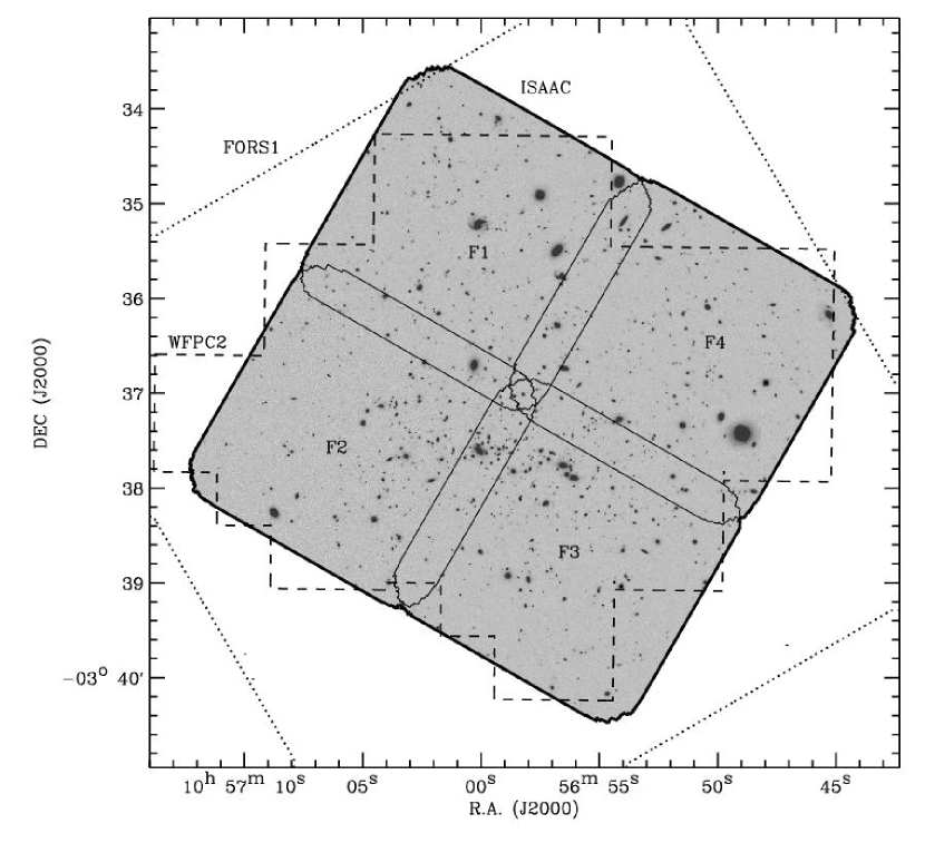
Figure 1.— Fields of view of $\rm MS\,1054-03$ covered by the different instruments. The full ISAAC field of view is outlined by the thick solid contour around the $K_{\rm s}$-band mosaic. The mosaic is normalized by the squared root of the weight map (§ 3.1) and displayed with a linear intensity scaling. The thin solid lines delineate the four individual ISAAC fields labeled F1 to F4, and show the regions of overlap. The dashed and dotted lines indicate the outer limits of the WFPC2 mosaic and the FORS1 field of view, respectively. The cluster is apparent as the east-west elongated S-shaped structure straddling fields F2 and F3.

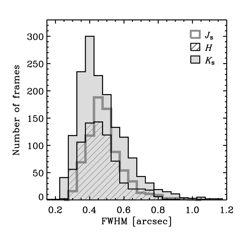
Figure 2.— Distributions of the seeing FWHM for the NIR ISAAC observations. The seeing was measured by fitting Moffat profiles to bright, isolated, unsaturated stars in the $\rm MS\,1054-03$ individual reduced frames. Histograms are shown for each band separately: $J_{\rm s}$ (empty histogram with thick grey line), $H$ (hatched histogram), and $K_{\rm s}$ (grey-filled histogram).

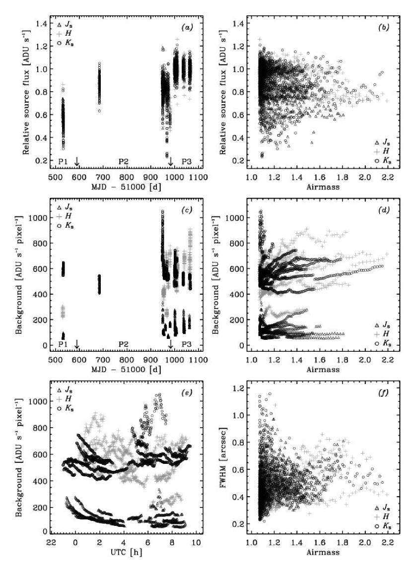
Figure 3.— Selected observational parameters for the NIR ISAAC data set. $J_{\rm s}$-, $H$-, and $K_{\rm s}$-band data are plotted with black triangles, grey crosses, and black cirlces, respectively. (a) Relative instrumental source count rates derived from bright stars in the $\rm MS\,1054-03$ field versus modified Julian date (in days). The arrows at the bottom of the plot indicate the February 2000 and March 2001 VLT Antu primary mirror realuminization, separating the periods P1, P2, and P3 of data acquisition. The count rates were integrated in a $6^{\prime\prime}$-diameter aperture and normalized to the median values over period P3. (b) Relative stars count rates versus airmass. (c) Background levels in the individual raw frames versus modified Julian date. The background corresponds to the median count rates in the raw frames. Periods P1 to P3 are identified at the bottom of the plot. (d) Background levels versus airmass. (e) Background levels versus Universal Time (in hours). (f) Seeing FWHM of individual frames versus airmass. In all plots some OBs depart from the general trends, reflecting particular conditions during the observations.

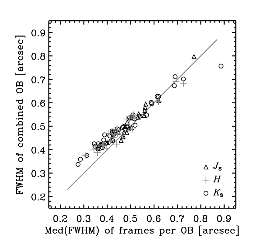
Figure 4.— Effects on the PSF of the combination and rectification of the ISAAC OB images. The FWHM of the PSF measured in the rectified combined OB images is compared to the median of the FWHMs in the individual non-rectified frames within each OB. The angular resolution is preserved to within $\pm 5\%$ at $\rm FWHM\geq 0\farcs 5$ and degrades progressively towards lower FWHM by up to 25% at $\approx 0\farcs 3$, at the limit of undersampling (see § 3.1). The FWHM was measured by fitting Moffat profiles to bright, isolated, unsaturated stars. Data are shown separately for the three NIR bands: $J_{\rm s}$: black triangles; $H$: grey crosses; $K_{\rm s}$: black circles.

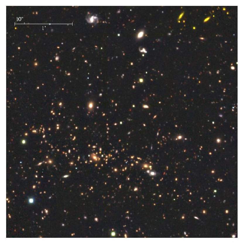
Figure 5.— Three-colour composite image of the central part of the $\rm MS\,1054-03$ field. The image is constructed from the WFPC2 $I_{814}$ map (coded in blue), and the ISAAC $J_{\rm s}$ and $K_{\rm s}$ maps (coded in green and red, respectively). All three maps are convolved to a common angular resolution of $\rm FWHM=0\farcs 69$ (the PSF of the $U$-band map, which has the poorest resolution among the full data set). The field of view shown is $4^{\prime}\times 4^{\prime}$; North is up and East is to the left. There is a rich variety of colours among the sources, especially for the fainter ones. Several of the red objects have spectroscopic or photometric redshift $z>2$, and are evolved, dust-obscured, massive galaxies (Förster Schreiber et al., 2004). Most are extremely faint in the observer’s optical bands and would be missed in optically-selected high-$z$ samples. The WFPC2 mosaic does not cover the top left and right corners, which causes the colours of many sources to appear yellow in these regions.

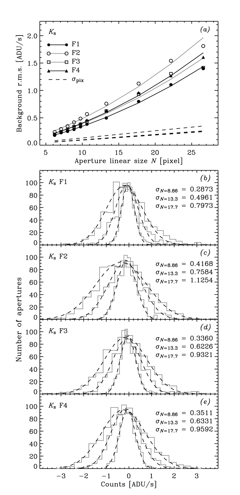
Figure 6.— Empirical scaling relation of the background noise rms of the $\rm MS\,1054-03$ field data set as a function of linear size $N=\sqrt{A}$ for apertures of area $A$. The plots show the relations for the four fields of the ISAAC $K_{\rm s}$-band mosaic used for the photometric measurements (rectified and resampled to the WFPC2 scale of $\rm 0\farcs 1~{}pixel^{-1}$ and smoothed to match the PSF of the FORS1 $U$-band data with $\rm FWHM=0\farcs 69$). The results are qualitatively similar for all other bands. (a) Measured rms variations of the background noise for different aperture sizes in each of the four ISAAC fields (F1: filled dots; F2: open dots; F3 : open squares; F4 : filled triangles). The solid lines indicate the best-fits to the measured relations following Eq. 3. The dashed lines show the linear predictions from the measured pixel-to-pixel rms if the noise were purely uncorrelated and Gaussian. (b), (c), (d), and (e) Distributions of count rates measured in random apertures within empty areas of the four ISAAC fields maps (histograms), which are used to determine the background noise rms for each aperture size. The histograms are plotted for three selected aperture sizes with $N=8.86$, 13.3, and 17.7 pixel, corresponding to circular apertures of diameters $d=1^{\prime\prime}$, $1\farcs 5$, and $2^{\prime\prime}$. The background noise rms is derived from the best-fit Gaussian profile to the distributions (black dashed lines).

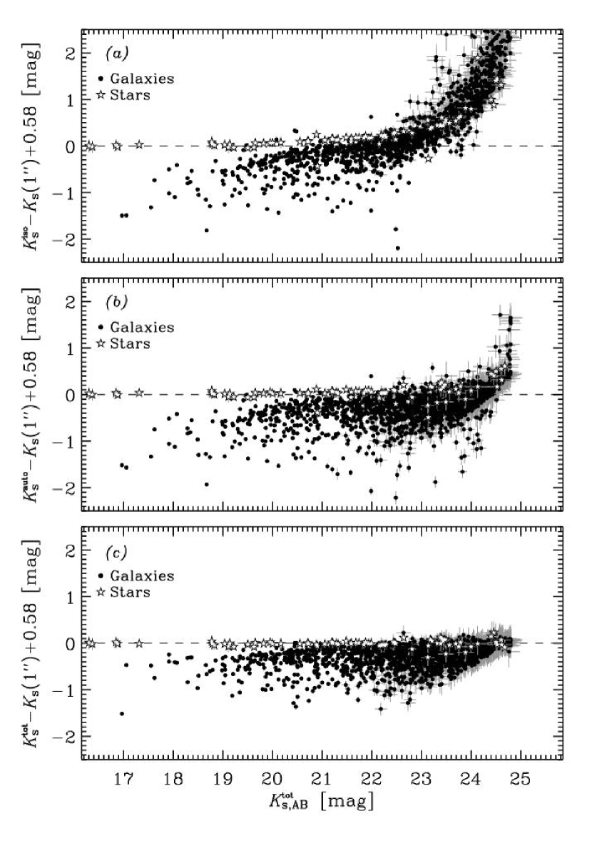
Figure 7.— Comparison of various methods to estimate total $K_{\rm s}$-band magnitudes. The plots show the difference between the various estimates and the expected total magnitude for point sources, given by the magnitude in a 1$\farcs$0-diameter circular aperture $K_{\rm s}(1^{\prime\prime})$ scaled by the total aperture correction of 0.58 mag (see § 5.2). The values of the abcsissa are our adopted total $K_{\rm s}$-band magnitudes. Stars are distinguished from galaxies (grey stars and black dots, respectively, see § 6). The error bars correspond to $1\sigma$ uncertainties. For point sources, the best $K^{\rm tot}_{s}$ estimates should be equal to $K_{\rm s}(1^{\prime\prime})-0.58$ over the entire range in brightness (horizontal black dashed lines). (a) Isophotal magnitudes $K^{\rm iso}_{\rm s}$ strongly underestimate the total magnitudes $K^{\rm tot}_{\rm s}$ at the faint end where most sources are point-like and where extended emission lies below the isophotal surface brightness threshold for detection and photometry. (b) Kron-like autoscaling magnitudes $K^{\rm auto}_{\rm s}$ still underestimate the $K^{\rm tot}_{\rm s}$ of the fainter objects by up to 0.58 mag, reflecting the emission missed from the PSF wings in the smaller apertures. (c) The turnover at faint magnitudes is nearly absent when using the $K^{\rm tot}_{s}$ as measured in this paper.

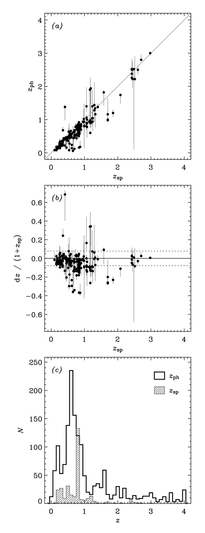
Figure 8.— Photometric and spectroscopic redshifts in the $\rm MS\,1054-03$ field. (a) Direct comparison between the photometric redshifts $z_{\rm ph}$ and spectroscopic redshifts $z_{\rm sp}$ for all $K_{\rm s}$-band detected sources at $K_{\rm s,AB}^{\rm tot}\leq 24.8~{}{\rm mag}$ for which a $z_{\rm sp}$ measurement is available. The vertical error bars indicate the 68% confidence intervals on $z_{\rm ph}$ derived from Monte-Carlo simulations (see § 6). In the ideal case, $z_{\rm ph}=z_{\rm sp}$ (grey solid line). (b) Residuals ${\rm d}z/(1+z_{\rm sp})\equiv(z_{\rm ph}-z_{\rm sp})/(1+z_{\rm sp})$ as a function of spectroscopic redshift. The accuracy of the photometric redshifts quantified by the mean $\langle|{\rm d}z|/(1+z_{\rm sp})\rangle$ is 0.078 (dotted lines) about the ideal value of 0 (solid line). (c) Distributions of photometric redshifts for all $K_{\rm s}$-band detected sources at $K_{\rm s,AB}^{\rm tot}\leq 24.8~{}{\rm mag}$ (hollow histogram) and of spectroscopic redshifts for the subset of objects for which they are available (grey filled histogram). In all plots, stars have been excluded.

Figure 9.— Results of the completeness simulations for point sources in the $K_{\rm s}$ band for the $\rm MS\,1054-03$ field. For the plots shown here, the analysis was carried out considering the entire area in each of the ISAAC fields with effective weight $w_{\rm F}>0.95$ including also the isophotal areas of real sources. (a) Completeness curves giving the fraction of recovered simulated sources as a function of input total $K_{\rm s}$-band magnitude. The results for each ISAAC field are plotted separately (black line and filled circles: F1; grey line and open circles: F2; grey line and open squares: F3; black line and filled triangles: F4). The 90% and 50% completeness limits are indicated (upper and lower dashed lines). (b) Observed versus input total $K_{\rm s}$-band magnitude for all artificial point sources in the simulations in all four ISAAC fields. The ideal relation where the observed magnitudes equal the input magnitudes is indicated (grey dashed line).

Figure 10.— Differential $K_{\rm s}$-band galaxy counts in the $\rm MS\,1054-03$ field. The counts are given as a function of the total $K_{\rm s}$-band AB magnitude (with total magnitudes computed as described in § 5.2). The raw counts (grey open circles) are summed up in bins 0.5 mag wide (plotted at the central bin values) and over the total area where each ISAAC field has an effective weight $w_{\rm F}$ exceeding 95% of its maximum. The counts were corrected for incompleteness (grey crosses) and for both incompleteness and spurious detections (black filled circles) using point-source simulations. Because the four fields have different noise properties, the corrections were derived and applied for each field separately, and further account for the variations of effective area as a function of depth. The corrections are small except in the faintest bin near the 50% completeness or $\approx 3\sigma$ detection limit (dashed vertical line). Correction for incompleteness only overestimates the counts at the faint end where the contribution from positive noise peaks becomes important. The counts at $K_{\rm s,AB}^{\rm tot}\approx 22-25~{}{\rm mag}$ ($\rm\approx 20-23.5$ in Vega magnitudes) have a logarithmic slope of $\alpha\approx 0.20$ (grey solid line). The error bars represent Poisson uncertainties. Galaxies from the $z=0.83$ cluster produce the bump seen around $K_{\rm s,AB}^{\rm tot}\approx 20.5~{}{\rm mag}$, as indicated by the number counts of sources around the cluster redshift (dotted line). Gravitational lensing by the cluster affects little the surface densities: the effects are small on average over the area surveyed and act along a direction roughly parallel to the counts curve as illustrated for the mean magnification by 20% for $z=2.5$ background source plane (arrow at bottom left; see § 8.2).

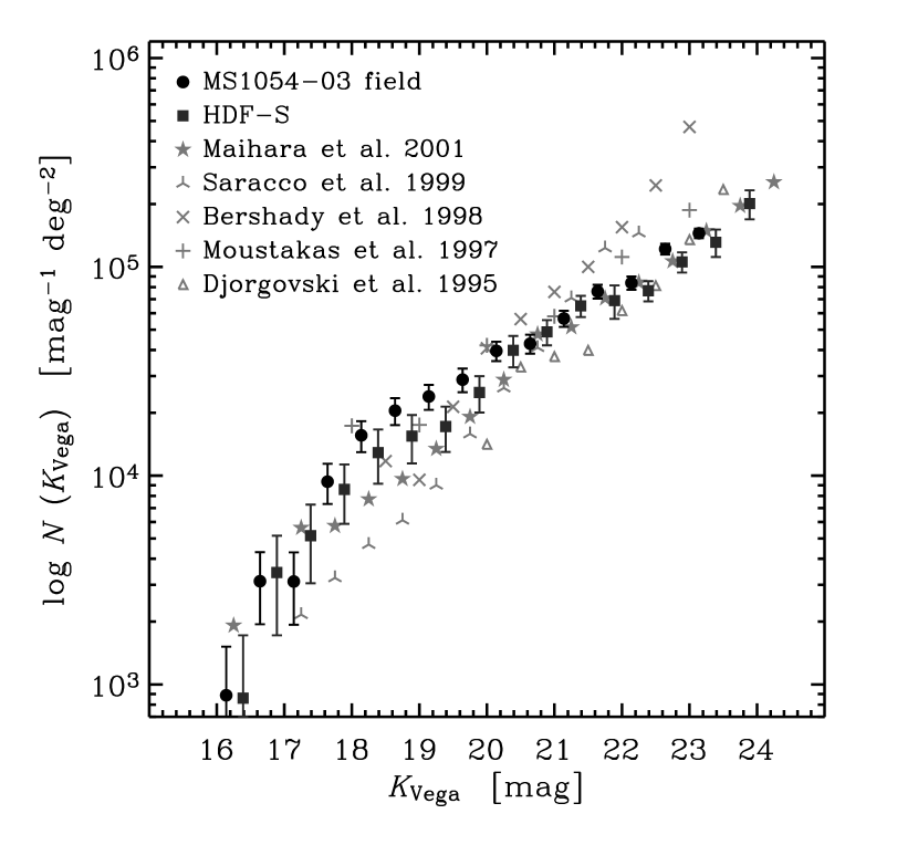
Figure 11.— FIRES $K_{\rm s}$-band galaxy counts compared to published counts in other deep $K$-band fields. All data are corrected counts, and are here plotted as a function of magnitudes in the Vega photometric system. The legend gives the symbols used for different references. All counts are plotted up to their $\approx 3\sigma$ detection or 50% completeness limits, except for the Saracco et al. (1999) data which extend to a $\rm S/N\approx 5$. Error bars are plotted for the FIRES counts and represent Poisson uncertainties. The $\approx 5$ times larger area of the $\rm MS1054-03$ field leads to more robust statistics than for the deeper but smaller HDF-S up to $K_{\rm Vega}\approx 23~{}{\rm mag}$, a depth only about 1 mag brighter than current deep $K$-band surveys. The cluster bump around $K_{\rm Vega}=18.5~{}{\rm mag}$ is conspicuous for the $\rm MS\,1054-03$ field. The counts slope at $K_{\rm Vega}>20~{}{\rm mag}$ in both FIRES fields lies generally at the flatter end of results reported in the literature. The differences between various surveys are probably due in part to field-to-field variations, and different methods used for the photometric measurements and for the derivation of the corrections to the raw counts.

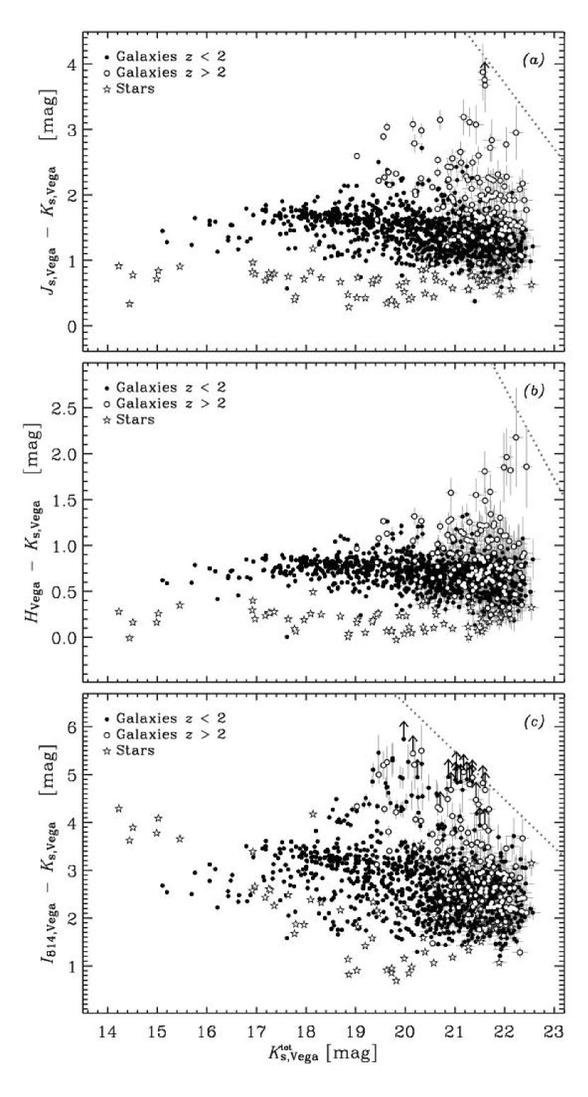
Figure 12.— Colour-magnitude diagrams of $K_{\rm s}$-band selected objects in the $\rm MS\,1054-03$ field. Magnitudes and colours are on the Vega system. Only sources with $\rm S/N>10$ on their $K_{\rm s}$-band colour flux and a minimum of 30% of the total exposure time in at least one ISAAC field for each NIR band and in the $I_{814}$-band map are included. Galaxies at $z<2$ and $z>2$ as well as stars are shown with different symbols (filled circles, open circles, and open stars, respectively). The error bars represent the $1\sigma$ photometric uncertainties, and sources with $\rm S/N<2$ in their $J_{\rm s}$-, $H$-, or $I_{814}$-band fluxes are plotted at their $2\sigma$ confidence level. The dotted line in each panel indicates the limits corresponding to the $3\sigma$ background noise level for the point-source aperture in the PSF-matched images used for the photometry. (a) $J_{\rm s}-K_{\rm s}$ colour versus total $K_{\rm s}$-band magnitude. (b) $H-K_{\rm s}$ colour versus total $K_{\rm s}$-band magnitude. (c) $I_{814}-K_{\rm s}$ colour versus total $K_{\rm s}$-band magnitude.

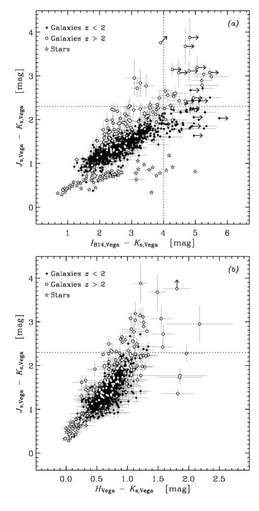
Figure 13.— Colour-colour diagrams of $K_{\rm s}$-band selected objects in the $\rm MS\,1054-03$ field. The colours are on the Vega system. Only sources with $\rm S/N>10$ on their $K_{\rm s}$-band colour flux and a minimum of 30% of the total exposure time in at least one ISAAC field for each NIR band and in the $I_{814}$-band map are included. Galaxies at $z<2$ and $z>2$ as well as stars are shown with different symbols (filled circles, open circles, and open stars, respectively). The error bars represent the $1\sigma$ photometric uncertainties, and sources with $\rm S/N<2$ in their $J_{\rm s}$-, $H$-, or $I_{814}$-band flux are plotted at their $2\sigma$ confidence level. (a) $J_{\rm s}-K_{\rm s}$ versus $I_{814}-K_{\rm s}$ colours. The criterion $J_{\rm s}-K_{\rm s}>2.3~{}{\rm mag}$ defined to identify Distant Red Galaxies at $z>2$ (DRGs; Franx et al., 2003) and the cutoff $I_{814}-K_{\rm s}>4.0~{}{\rm mag}$ to select Extremely Red Objects (EROs) are indicated (horizontal and vertical dotted lines, respectively). (b) $J_{\rm s}-K_{\rm s}$ versus $H-K_{\rm s}$ colours. The criterion $J_{\rm s}-K_{\rm s}>2.3~{}{\rm mag}$ to select DRGs at $z>2$ is again indicated (horizontal dotted line).

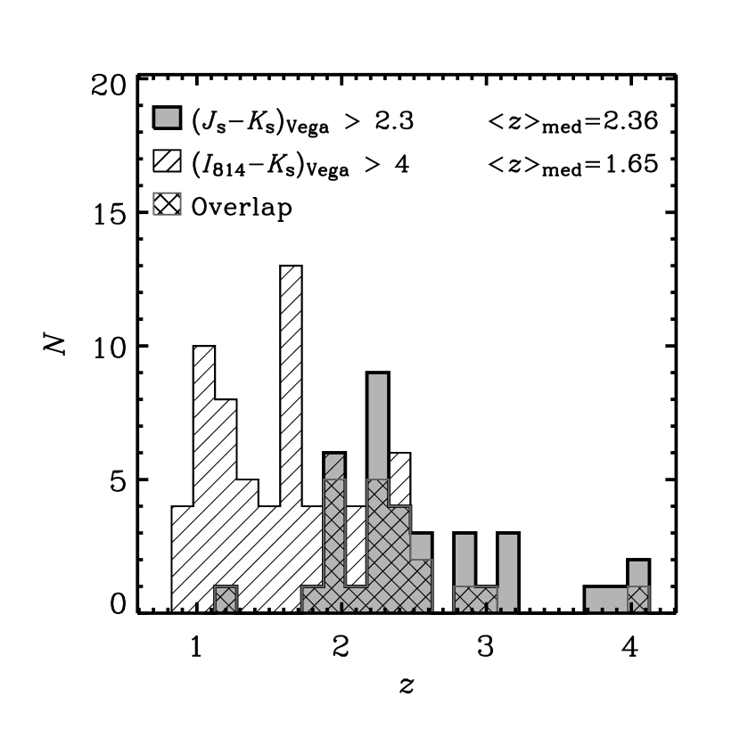
Figure 14.— Redshift distributions of red $K_{\rm s}$-band selected galaxies in the $\rm MS\,1054-03$ field. Only galaxies with $\rm S/N>10$ on their $K_{\rm s}$-band colour flux (implying $K_{\rm s,Vega}^{\rm tot}\leq 22.5~{}{\rm mag}$) and a minimum of 30% of the total exposure time in at least one ISAAC field for each NIR band and in the $I_{814}$-band map are included. The spectroscopic redshifts were used wherever available. The colour cut $J_{\rm s,Vega}-K_{\rm s,Vega}>2.3~{}{\rm mag}$ is devised to identify evolved galaxies at $z>2$ (Distant Red Galaxies or DRGs; Franx et al. 2003). The galaxies that satisfy this criterion (filled histogram) all lie at $z>1.8$ except for one interloper at $z=1.19$, with median redshift $\langle z\rangle_{\rm med}=2.36$ (2.42 when excluding the interloper). The galaxies that have $I_{814,Vega}-K_{\rm s,Vega}>4$ colours of Extremely Red Objects (EROs; hatched histogram) typically lie at lower redshifts, with $\langle z\rangle_{\rm med}=1.65$. There is overlap between the two colour-selected samples (cross-hatched histogram) but the $J_{\rm s,Vega}-K_{\rm s,Vega}>2.3$ criterion selects more efficiently $z>2$ galaxies.

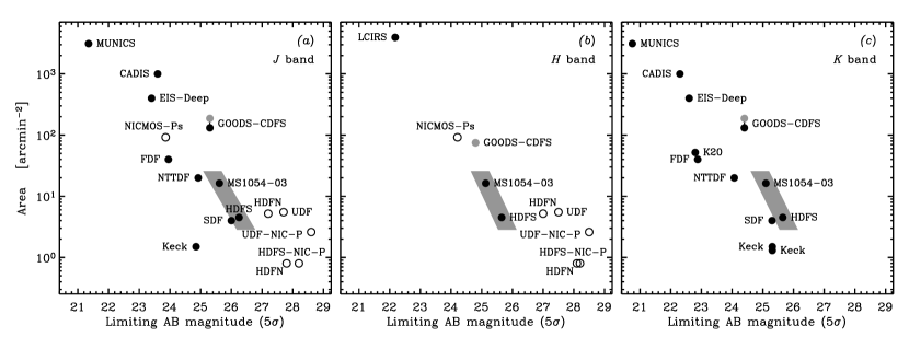
Figure 15.— Comparison of published deep NIR imaging surveys in the literature as a function of depth and area. (a) $J$-band surveys, including HST NICMOS imaging in the F110W bandpass. (b) $H$-band surveys, including HST NICMOS imaging in the F160W bandpass. (c) $K$-band surveys, including imaging with $K$, $K_{\rm s}$, and $K^{\prime}$ filters. Ground-based and space-based surveys are distinguished by different symbols (filled circles and open circles, respectively). In addition to the FIRES HDF-S and $\rm MS\,1054-03$ fields (highlighted by the shaded area), the surveys considered include the following: the NICMOS fields of the HDF-N (HDFN, from Thompson et al. 1999 for the deeper but smaller area, and from Dickinson et al. 2003 for the wider and shallower area); the NICMOS field of the Hubble Ultra Deep Field (UDF, Thompson et al., 2005); the HDF-S parallel NICMOS field (HDFS-NIC-P, Williams et al., 2000); the two UDF parallel NICMOS fields (UDF-NIC-P, Bouwens et al., 2005); the Subaru Deep Field (SDF, Maihara et al., 2001); several blank fields imaged with the Keck telescopes (three fields in $K$ from Djorgovski et al. 1995 and two in $J$ and $K$ from Bershady et al. 1998); the Chandra Deep Field South as part of GOODS (GOODS-CDFS, Giavalisco et al., 2004); the ESO New Technology Telescope Deep Field (NTTDF, Saracco et al., 1999); the FORS Deep Field (FDF, Heidt et al., 2003); the NICMOS parallel imaging database for Cycle 7 of high Galactic latitude fields (NICMOS-Ps, Corbin et al., 2000); the two fields as basis for the K20 survey (Cimatti et al., 2002); the ESO Imaging Survey Deep fields (EIS-Deep, Arnouts et al., 2001); the Calar Alto Deep Imaging Survey (CADIS, Meisenheimer, 1998); the Las Campanas Infrared Survey (LCIRS, Chen et al., 2002); the Munich Near-Infrared Cluster Survey (MUNICS, Drory et al., 2001). For GOODS-CDFS, we used the average depth reported by ESO for the version 1.0 public release of the NIR ISAAC data covering $\rm 131~{}arcmin^{2}$ in $J$ and $K_{\rm s}$ (shown in black); the expected area and additional $H$-band data once the survey is completed are also indicated (grey filled circle). As much as possible, the limiting depths refer to total magnitudes, or magnitudes in fixed apertures significantly larger than the PSF, for point sources. The FIRES data of HDF-S currently represents the deepest ground-based survey in the $J$ and $H$ bands, and the deepest survey in the $K$ band from either ground or space. The wider FIRES $\rm MS\,1054-03$ field is the deepest for its size, filling the regime between the ultra-deep surveys over smaller areas and significantly larger but yet shallower fields such as GOODS-CDFS.

Table 1Summary of the $\rm MS\,1054-03$ field observations

Camera	Filter	Pointings	$N_{\rm exp}$	$t_{\rm int}$	PSF
				(s)	(arcsec)
All bands
FORS1	$U$	1	30	16500	0.69
FORS1	$B$	1	18	7200	0.57
FORS1	$V$	1	6	1800	0.65
WFPC2	F606W	6	12	6500	0.21
WFPC2	F814W	6	12	6500	0.22
ISAAC	$J_{\rm s}$	4	776	93120	0.48
ISAAC	$H$	4	739	87780	0.46
ISAAC	$K_{\rm s}$	4	1588	95280	0.52
Near-infrared bands
ISAAC	$J_{\rm s}$	F1	205	24600	0.44
		F2	211	25320	0.46
		F3	180	21600	0.45
		F4	180	21600	0.46
ISAAC	$H$	F1	196	23520	0.46
		F2	180	20700	0.42
		F3	184	22080	0.43
		F4	179	21480	0.42
ISAAC	$K_{\rm s}$	F1	473	28380	0.46
		F2	398	23880	0.50
		F3	358	21480	0.41
		F4	359	21540	0.39

Table 2Adopted photometric zero points for the $\rm MS\,1054-03$ data set

Data set	Zero point
	Vega mag	AB mag
FORS1 $U$	24.127	24.828
FORS1 $B$	26.746	26.634
FORS1 $V$	27.131	27.145
WFPC2 $V_{606}$	22.900	23.020
WFPC2 $I_{814}$	21.660	22.090
ISAAC $J_{\rm s}$	24.970	25.872
ISAAC $H$	24.846	26.226
ISAAC $K_{\rm s}$	24.309	26.169

Note. — FORS1 and ISAAC measurements were performed in a 6″-diameter circular aperture. WFPC2 values refer to an “infinite” aperture, which is defined as having 1.096 times the flux in an aperture 0$\farcs$5 in radius. The zero points for the FORS1 optical bands were derived applying $m_{\rm Vega}=m_{\rm instr}+{\rm ZP_{Vega}}-\kappa\cdot z+\gamma_{\rm C}\cdot{\rm C_{Vega}}$, where $m_{\rm Vega}$ is the calibrated magnitude of the standard star, $m_{\rm instr}=-2.5\,\log({\rm counts~{}rate})$ is the instrumental magnitude, $z$ is the airmass, and $\rm C$ is the reference colour for the colour term. The extinction coefficients used were $\kappa(U)=0.41$, $\kappa(B)=0.21$, and $\kappa(V)=0.16$, in units of $\rm mag\,airmass^{-1}$. The colour coefficients were $\gamma_{U-B}(U)=0.10$, $\gamma_{B-V}(B)=-0.09$, and $\gamma_{B-V}(V)=0.05$. Extinction and colour terms were not applied for the ISAAC zero points as explained in § 3.1. The WFPC2 zero points were directly taken from the WFPC2 manual.

Table 3Background noise in the PSF-matched $\rm MS\,1054-03$ field images

Data set		$\overline{\sigma}$	$a$	$b$	$1\sigma$ background noise limit in $d=1\farcs 035$
		(counts/s)			(AB mag)
FORS1 $U$		$1.13\times 10^{-3}$	1.82	0.025	29.01
FORS1 $B$		$2.25\times 10^{-3}$	2.31	0.093	29.60
FORS1 $V$		$9.24\times 10^{-3}$	2.30	0.034	28.78
WFPC2 $V_{606}$		$1.23\times 10^{-4}$	2.01	0.234	28.84
WFPC2 $I_{814}$		$1.01\times 10^{-4}$	2.19	0.224	28.10
ISAAC $J_{\rm s}$	F1	0.00504	2.57	0.121	27.80
	F2	0.00591	2.13	0.140	27.70
	F3	0.00531	1.96	0.143	27.87
	F4	0.00489	2.65	0.109	27.84
ISAAC $H$	F1	0.01054	3.29	0.101	27.20
	F2	0.01192	2.79	0.128	27.14
	F3	0.00957	3.06	0.111	27.34
	F4	0.00939	2.71	0.136	27.40
ISAAC $K_{\rm s}$	F1	0.00926	2.45	0.128	27.45
	F2	0.01323	2.54	0.115	27.07
	F3	0.00985	2.76	0.125	27.30
	F4	0.00975	2.73	0.143	27.28

Table 4Background noise in the non PSF-matched $\rm MS\,1054-03$ field images

Data set		Point-source aperture diameter	$1\sigma$ limiting depth	$3\sigma$ total limiting magnitude
		(arcsec)	(AB mag)	(AB mag)
FORS1 $U$		1.035	29.01	27.24
FORS1 $B$		1.035	29.60	27.83
FORS1 $V$		1.035	28.78	27.01
WFPC2 $V_{606}$		0.31	30.00	28.28
WFPC2 $I_{814}$		0.33	29.24	27.46
ISAAC $J_{\rm s}$	F1	0.72	28.00	26.20
	F2	0.72	27.77	25.97
	F3	0.72	27.95	26.15
	F4	0.72	27.98	26.18
ISAAC $H$	F1	0.69	27.39	25.57
	F2	0.69	27.31	25.49
	F3	0.69	27.61	25.79
	F4	0.69	27.63	25.81
ISAAC $K_{\rm s}$	F1	0.78	27.61	25.73
	F2	0.78	27.16	25.28
	F3	0.78	27.50	25.63
	F4	0.78	27.54	25.67

Table 5$K_{\rm s}$-band completeness limits for the $\rm MS\,1054-03$ field

Field	All image area		Masking real sources
	90% limit	50% limit	90% limit	50% limit
	(AB mag)	(AB mag)	(AB mag)	(AB mag)
F1	24.33	25.30	24.76	25.34
F2	23.91	25.31	24.60	25.36
F3	23.73	25.29	24.64	25.32
F4	24.51	25.31	24.73	25.34

References

- Amico et al. (2002) Amico, P., Cuby, J.-G., Devillard, N., Yung, Y., & Lidman, C. 2002, ISAAC Data Reduction Guide, Version 1.5, (Garching: ESO)
- Appenzeller et al. (1998) Appenzeller, I., et al. , 1998, The Messenger, 94, 1
- Arnouts et al. (2001) Arnouts, S., et al. , 2001, A&A, 379, 740
- Bershady et al. (1998) Bershady, M. A., Lowenthal, J. D., & Koo, D. C. 1998, ApJ, 505, 50
- Bertin & Arnouts (1996) Bertin, E., & Arnouts, S. 1996, A&AS, 117, 393
- Best et al. (2002) Best, P., van Dokkum, P. G., Franx, M., & Röttgering, H. J. A. 2002, MNRAS, 330, 17
- Bouwens et al. (2005) Bouwens, R. J., Illingworth, G. D., Thompson, R. I., & Franx, M. 2005, ApJ, 624, L5
- Casali & Hawarden (1992) Casali, M., & Hawarden, T. 1992, JCMT-UKIRT Newsl., No. 4, 33
- Chen et al. (2002) Chen, H.-W., et al. , 2002, ApJ, 570, 54
- Cimatti et al. (2002) Cimatti, A., et al. , 2002, A&A, 392, 395
- Corbin et al. (2000) Corbin, M. R., O’Neil, E., Thompson, R. I., Rieke, M. J., & Schneider, G. 2000, AJ, 120, 1209
- Daddi et al. (2003) Daddi, E., et al. , 2003, ApJ, 588, 50
- Dickinson et al. (2003) Dickinson, M., et al. , 2003, in preparation
- Djorgovski et al. (1995) Djorgovski, S., et al. , 1995, ApJ, 438, L13
- Drory et al. (2001) Drory, N., Feulner, G., Bender, R., Botzler, C. S., Hopp, U., Maraston, C., Mendes de Oliveira, C., & Snigula, J. 2001, MNRAS, 325, 550
- Förster Schreiber et al. (2004) Förster Schreiber, N. M., et al. , 2004, ApJ, 616, 40
- Franx et al. (2000) Franx, M., et al. , 2000, The Messenger, 99, 20
- Franx et al. (2003) Franx, M., et al. , 2003, ApJ, 587, L79
- Giavalisco et al. (2004) Giavalisco, M., et al. , 2004, ApJ, 600, L93
- Hauschildt et al. (1999) Hauschildt, P. H., Allard, F., Ferguson, J., Baron, E., & Alexander, D. R. 1999, ApJ, 525, 871
- Heidt et al. (2003) Heidt, J., et al. , 2003, A&A, 398, 49
- Hoekstra et al. (2000) Hoekstra, H., Franx, M., & Kuijken, K. 2000, ApJ, 532, 88
- Jeltema et al. (2001) Jeltema, T. E., Canizares, C. R., Bautz, M. W., Malm, M. R., Donahue, M., & Garmire, G. P. 2001, ApJ, 562, 124
- Kron (1980) Kron, R. G. 1980, ApJS, 43, 305
- Kuchinski et al. (2001) Kuchinski, L. E., Madore, B. F., Freedman, W. L., & Trewhella, M. 2001, AJ, 122, 729
- Labbé et al. (2003a) Labbé, I., et al. , 2003a, AJ, 125, 1107
- Labbé et al. (2003b) Labbé, I., et al. , 2003b, ApJ, 591, L95
- Labbé et al. (2005) Labbé, I., et al. , 2005, ApJ, 624, L81
- Landolt (1992) Landolt, A. U. 1992, AJ, 104, 340
- Madau (1995) Madau, P. 1995, ApJ, 441, 18
- Maihara et al. (2001) Maihara, T., et al. , 2001, PASJ, 53, 25
- McCarthy (2004) McCarthy, P. J., 2004, ARA&A, 42, 477
- Meisenheimer (1998) Meisenheimer, K. 1998, Astronomische Gesellschaft Meeting Abstracts, 14, 3
- Monet et al. (1998) Monet, D. G., et al. , 1998, VizieR Online Data Catalog, I/252
- Moorwood et al. (1998) Moorwood, A. F. M., et al. , 1998, The Messenger, 94, 7
- Moustakas et al. (1997) Moustakas, L. A., Davis, M., Graham, J. R., Silk, J., Peterson, B. A., & Yoshii, Y. 1997, ApJ, 475, 445
- Oke (1971) Oke, J. B. 1971, ApJ, 170, 193
- Papovich et al. (2001) Papovich, C., Dickinson, M., & Ferguson, H. C. 2001, ApJ, 559, 620
- Persson et al. (1998) Persson, S. E., Murphy, D. C., Krzeminski, W., Roth, M., & Rieke, M. J. 1998, AJ, 116, 2475
- Rubin et al. (2004) Rubin, K. H. R., van Dokkum, P. G., Coppi, P., Johnson, O., Förster Schreiber, N. M., Franx, M., & van der Werf, P. 2004, ApJ, 613, L5
- Rudnick et al. (2001) Rudnick, G., et al. , 2001, AJ, 122, 2205
- Rudnick et al. (2003) Rudnick, G., et al. , 2003, ApJ, 599, 847
- Saracco et al. (1999) Saracco, P., D’Odorico, S., Moorwood, A. F. M., Buzzoni, A., Cuby, J.-G., & Lidman, C. 1999, A&A, 349, 751
- Shapley et al. (2001) Shapley, A. E., Steidel, C. C., Adelberger, K. L., Dickinson, M., Giavalisco, M., & Pettini, M. 2001, ApJ, 562, 95
- Thompson et al. (1999) Thompson, R. I., Storrie-Lombardi, L. J., Weymann, R. J., Rieke, M. J., Schneider, G., Stobie, E., & Lytle, D. 1999, AJ, 117, 17
- Thompson et al. (2005) Thompson, R. I., et al. , 2005, AJ, in press (astro-ph/0503504)
- Tran et al. (2003) Tran, K.-V. H., et al. , 2003, in preparation
- Tran et al. (1999) Tran, K.-V. H., Kelson, D. D., van Dokkum, P. G., Franx, M., Illingworth, G. D., & Magee, D. 1999, ApJ, 522, 39
- Trujillo et al. (2003) Trujillo, I. et al., 2003, ApJ, 604, 521
- Trujillo et al. (2005) Trujillo, I. et al., 2005, ApJ, submitted (astro-ph/0504225)
- Toft et al. (2005) Toft, S., van Dokkum, P. G., Franx, M., Thompson, R. I., Illingworth, G. D., Bouwens, R. J., & Kriek, M. 2005, ApJ, 624, L9
- van Dokkum (2001) van Dokkum, P.G. 2001, PASP, 113, 1420
- van Dokkum et al. (2000) van Dokkum, P.G., Franx, M., Fabricant, D., Illingworth, G.D., & Kelson, D.D. 2000, ApJ, 541, 95
- van Dokkum et al. (2005) van Dokkum, P. G., Kriek, M., Rodgers, B., Franx. M., & Puxley, P. 2005, ApJ, 622, L13
- van Dokkum et al. (2003) van Dokkum, P. G., et al. 2003, ApJ, 587, L83
- van Dokkum et al. (2004) van Dokkum, P. G., et al. 2004, ApJ, 611, 703
- Warmels (1991) Warmels, R. H., 1991, “The ESO-MIDAS System,” in Astronomical Data Analysis Software and Systems I (PASP Conf. Series), 25, 115
- Williams et al. (2000) Williams, R. E., et al. , 2000, AJ, 120, 2735
- Zacharias et al. (2004) Zacharias, N., Urban, S. E., Zacharias, M. I., Wycoff, G. L., Hall, D. M., Germain, M. E., Holdenried, E. R., & Winter, L. 2004, AJ, 127, 3043