Axisymmetric simulations of magneto–rotational core collapse:
dynamics and gravitational wave signal

Abstract

Aims. We have performed a comprehensive parameter study of the collapse of rotating, strongly magnetized stellar cores in axisymmetry to determine their gravitational wave signature based on the Einstein quadrupole formula.

Methods. We use a Newtonian explicit magnetohydrodynamic Eulerian code based on the relaxing-TVD method for the solution of the ideal MHD equations, and apply the constraint-transport method to guarantee a divergence–free evolution of the magnetic field. We neglect effects due to neutrino transport and employ a simplified equation of state. The initial models are polytropes in rotational equilibrium with a prescribed degree of differential rotation and rotational energy. The initial magnetic fields are purely poloidal the field strength ranging from $10^{10}\mathrm{G}$ to $10^{13}\mathrm{G}$. The evolution of the core is followed until a few ten milliseconds past core bounce.

Results. The initial magnetic fields are amplified mainly by the differential rotation of the core giving rise to a strong toroidal field component with an energy comparable to the rotational energy. The poloidal field component grows by compression during collapse, but does not change significantly after core bounce. In large parts of the simulated cores the growth time of the magneto–rotational instability (MRI) is of the order of a few milliseconds. The saturation field strengths that can be reached both via a pure $\Omega$ dynamo or the MRI are of the order of $10^{15}\mathrm{G}$ at the surface of the core. Sheet-like circulation flows which produce a strong poloidal field component transporting angular momentum outwards develop due to MRI, provided the initial field is not too weak. Weak initial magnetic fields ($\la 10^{11}\mathrm{G}$) have no significant effect on the dynamics of the core and the gravitational wave signal. Strong initial fields ($\ga 10^{12}\mathrm{G}$) cause considerable angular momentum transport whereby rotational energy is extracted from the collapsed core which loses centrifugal support and enters a phase of secular contraction. The gravitational wave amplitude at bounce changes by up to a few ten percent compared to the corresponding non-magnetic model. If the angular momentum losses are large, the post–bounce model. If the angular momentum losses are large the post–bounce equilibrium state of the core changes from a centrifugally to a pressure supported one. This transition imprints in the gravitational wave signal a reduction of the amplitude of the large–scale oscillations characteristic of cores bouncing due to centrifugal forces.

In some models the quasi-periodic large-scale oscillations are replaced by higher frequency irregular oscillations. This pattern defines a new signal type which we call a type IV gravitational wave signal. Collimated bipolar outflows give rise to a unique feature that may allow their detection by means of gravitational wave astronomy: a large positive quadrupole wave amplitude of similar size as that of the bounce signal.

1 Introduction

The gravitational binding energy liberated by the collapse of the iron core of a massive ($M\ga 8\ M_{\odot}$) star to a neutron star is the commonly accepted energy source of type Ib/c and type II supernovae, as a few percent of this energy are sufficient to unbind and rapidly eject the stellar envelope and to create the supernova outburst. However, which physical processes turn the central implosion into the explosion of the stellar layers surrounding the forming neutron star is still debated in spite of many efforts over more than three decades. Heating of stellar gas just outside the proto–neutron star (PNS) by neutrinos diffusing and being advected out of its interior is thought to play a crucial role in the explosion mechanism. However, as current neutrino–driven supernova models produce (weak) explosions only for low mass progenitors (for a recent review, see e.g. Janka et al., 2004), there may be a need to include additional physics in the models in order to make them work successfully for more massive progenitors, too.

On this account magneto–rotational core collapse, which has been studied by a few authors in the past (LeBlanc & Wilson, 1970; Bisnovatyi-Kogan et al., 1976; Meier et al., 1976; Müller & Hillebrandt, 1979; Ohnishi, 1983; Symbalisty, 1984), has become an active research field in recent years (Wheeler et al., 2002; Akiyama et al., 2003; Kotake et al., 2004a, b; Takiwaki et al., 2004; Wheeler & Akiyama, 2004; Yamada & Sawai, 2004; Ardeljan et al., 2005; Kotake et al., 2005; Sawai et al., 2005). Further reasons for this activity are the availability of sufficient computational power for the necessarily multi–dimensional magneto-hydrodynamic (MHD) simulations, observations indicating very asymmetric explosions (Wang et al., 1996, 2001; Leonard et al., 2001), and the interpretation of Anomalous X-Ray Pulsars and Soft Gamma-Ray Repeaters as magnetars, i.e. very strongly magnetized neutron stars (Duncan & Thompson, 1992; Thompson & Duncan, 1996; Kouveliotou et al., 1999).

Concerning the initial conditions for magneto–rotational core collapse the up to now most advanced evolutionary calculations of rotating massive stars (Heger et al., 2005) predict that the initial rotation rates are more than an order of magnitude smaller than (i) the minimum ones used in past (parameter) studies of magneto–rotational core collapse, and (ii) those predicted by previous evolutionary calculations (see, e.g. Woosley et al., 2002; Hirschi et al., 2003) which lead to neutron stars rotating very rapidly ($\sim 1\,$ms) at birth. The latter studies ignored the torques exerted in differentially rotating regions by the magnetic fields that thread them. Thus, the stars end up with 30 to 50 times more angular momentum than in the models by Heger et al. (2005) in that part of their core destined to collapse to a neutron star.

The strength (and distribution) of the initial magnetic field in the stellar core is unknown. If weak initially, several possible amplification mechanisms exist that may amplify the magnetic field of the collapsing progenitor to a dynamically important strength. Linear amplification of the field by means of differential rotation will occur Meier et al. (1976), which transforms rotational energy into magnetic energy by winding up any seed polodial field into a toroidal magnetic field. This process can be accompanied by the action of meridional (e.g. convective) motions that transform toroidal into poloidal fields. Both processes together lead to the so–called $\alpha$-$\Omega$ dynamo. Recently, the magneto-rotational instability (MRI) (see Balbus & Hawley, 1998) has received a lot of interest in the context of supernova collapse and explosion (Akiyama et al., 2003; Kotake et al., 2004a; Yamada & Sawai, 2004; Sawai et al., 2005). Unlike linear wrapping, the MRI will give rise to an exponential growth of the field strength while working on the same time scale (see however Sawai et al., 2005). The MRI saturation field is independent of the initial field, i.e. even quite small initial fields can be amplified to dynamically important strengths. The MRI will occur if the radial gradient of the angular velocity is negative, a condition arising quite naturally in core collapse situations.

A major effect of magnetic fields on the collapse dynamics is the transport of angular momentum. Due to its very low (fluid and $\nu$ shear) viscosity (see e.g. Keil et al., 1996) a collapsing non–magnetized stellar core maintains its Lagrangian angular momentum profile $\@vec{j}(m)$, $m$ being the Lagrangian mass coordinate, on time scales of $\sim 1\,$s, but magnetic fields can significantly redistribute the angular momentum (Meier et al., 1976). This can slow down the forming neutron star and thus counteract the effects of rotation. In some cases, even retrograde rotation may result in some parts of the core (Müller & Hillebrandt, 1979). Angular momentum transfer can also destabilize the rotational equilibrium the core resides in after a centrifugal bounce at sub–nuclear densities, and lead to a subsequent (second) collapse to nuclear densities and beyond that releases large amounts of gravitational binding energy (Symbalisty, 1984). Conversely, the violent convective flow both inside the neutrino sphere and between the neutrino sphere and the shock will transport and amplify magnetic fields in the collapsed core of a supernova (Thompson & Murray, 2001)

Analytic considerations (Meier et al., 1976; Wheeler et al., 2002) and numerical simulations (LeBlanc & Wilson, 1970; Symbalisty, 1984; Akiyama et al., 2003; Kotake et al., 2004b, a; Yamada & Sawai, 2004; Ardeljan et al., 2005; Sawai et al., 2005) show that magneto-rotational core collapse might lead to jet–like explosions. Though the magnetic stress will remain below equipartition strength in most regions of the star, it might affect the dynamics of the core through its anisotropic components. Magnetic stresses can assist in pushing the stalled shock, or may even drive a mildly relativistic outflow in form of a jet along the rotation axis, which is powered by the rotational energy transfered to the jet by the magnetic stresses.

Observations of gravitational waves (GWs) will allow one to learn more about the supernova mechanism as they provide pristine information directly from the stellar interior, in particular about the amount and distribution of the angular momentum, and the strength and topology of the magnetic field. Simplified Newtonian (Mueller, 1982; Mönchmeyer et al., 1991; Yamada & Sato, 1994; Zwerger & Müller, 1997; Kotake et al., 2003, 2004b; Fryer et al., 2004; Ott et al., 2004; Yamada & Sawai, 2004) and general–relativistic (Dimmelmeier et al., 2002a, b) calculations of rotational core collapse predict the emission of a strong signal around core bounce, and that the magnitude of the bounce signal as well as the post–bounce gravitational radiation depend sensitively on the initial rotation rate and rotation profile. Newtonian hydrodynamic simulations using more sophisticated micro- and transport–physics, as well as state–of–the–art rotating progenitors (Heger et al., 2005) show that the gravitational wave signal at core bounce is small compared to the signal produced by convective motions in the post–bounce core and by aspheric neutrino emission Müller et al. (2004). Magneto-rotational effects on the gravitational wave signature were first investigated in detail by Kotake et al. (2004b) and Yamada & Sawai (2004) who found differences from the signature of purely hydrodynamic models only in the case of very strong initial fields ($|\@vec{B}|\ga 10^{12}\mathrm{G}$).

In the following we present a comprehensive parameter study of the axisymmetric Newtonian core collapse of rotating magnetized polytropes and of their gravitational wave signature. Our study extends the work of Zwerger & Müller (1997) (hereafter ZM) and the complementary work of Dimmelmeier et al. (2002a, b) (hereafter DFM), who investigated the hydrodynamic collapse of a large set of rotating polytropes in Newtonian and general relativistic gravity, respectively. The simulations have been performed with the recently developed MHD difference scheme of Pen et al. (2003). They incorporate neither neutrino transport nor nuclear burning processes. Due to the reduced complexity of our models we could explore many of them covering a large region in parameter space, the focus being the gravitational wave signal emitted by magnetized stellar cores and their dynamic evolution. Because of our assumptions and approximations the validity of our models is limited to the stage of core collapse and to the first few ten milliseconds of their post–bounce evolution.

Several related but less comprehensive numerical MHD studies have been performed in the past few years: Yamada & Sawai (2004) used the ZEUS-2D code, employed the parametric equation of state of Yamada & Sato (1994), considered no neutrinos, and followed the evolution of initially rapidly rotating and very strongly magnetized ($|\@vec{B}|\ga 10^{12}\mathrm{G}$ cores with a purely homogeneous poloidal field. Contrary to LeBlanc & Wilson (1970) and Symbalisty (1984) they find that the magnetic field becomes strongest behind the shock wave and not in the inner core, and thus is the main driving factor of the observed jet outflow along the rotation axis. Besides a field amplification by differential rotation, they also observe the possible action of the MRI. They calculate the gravitational wave signal in the quadrupole approximation finding no substantial difference between the bounce signal of magnetized and non–magnetized models. Kotake et al. (2004b) also use the ZEUS-2D code to which they add an approximate neutrino cooling with a leakage scheme. They assume an initially predominantly toroidal magnetic field in their investigated 14 models of which all but one are very strongly magnetized $|\@vec{B}|>10^{11}\mathrm{G}$. Besides the simplified equation of state of Yamada & Sato (1994) they also consider two realistic equations of state. Kotake et al. (2004b) focus their study on the effect of the magnetic field on the gravitational wave signal, and find that the gravitational wave amplitudes are lowered by $\sim 10\%$ for models with the strongest initial magnetic fields ($|\@vec{B}|\sim 10^{14}\mathrm{G}$). Kotake et al. (2004a), Takiwaki et al. (2004), and Kotake et al. (2005) all using the same input physics and numerics as Kotake et al. (2004b) are concerned with the effects of the magnetic fields on the anisotropic neutrino radiation and convection, on the propagation of the shock wave, and on the rotation–induced anisotropic neutrino heating through parity–violating effects, respectively. Kotake et al. (2004a) find that the aspherical shapes of the shock and of the neutrino sphere (oblate or prolate depending on the initial rotation law) are enhanced in the magnetized models, and that the MRI is expected to develop on the prompt shock propagation time scale. Takiwaki et al. (2004) observe the formation of a tightly collimated shock wave along the rotational axis for strongly magnetized models. Kotake et al. (2005) find an at most 0.5% change of the neutrino heating rates even in their most strongly magnetized models ($|\@vec{B}|\ga 10^{13}\mathrm{G}$). Ardeljan et al. (2005) employ a 2D implicit Lagrangian code, a simplified equation of state, and consider energy losses by neutrinos and iron dissociation. They add a magnetic field of quadrupole–like symmetry with an energy of $10^{-6}$ of the core’s gravitational binding energy to the collapsed, post–bounce differentially rotating, stationary core. The toroidal field component of this seed field first grows linearly due to differential rotation, but then starts to amplify exponentially due to the action of the MRI. The resulting drastic increase of the magnetic pressure eventually causes an explosion with an energy of $0.6\,10^{51}\,$erg. Finally, Sawai et al. (2005) extend the work of Yamada & Sawai (2004) by considering inhomogeneously magnetized cores mainly in the very strong field regime ($|\@vec{B}|\sim 10^{12}\mathrm{G}\ldots 10^{13}\mathrm{G}$), which may produce magnetars. They find that poloidal magnetic fields which are initially concentrated toward the rotation axis produce more energetic explosions and more prolate shocks than cores with an initially uniform field. A core with an initially quadrupolar field (Ardeljan et al., 2005) gives rise to a collimated fast jet ($v\la c/2$), while a core with a pure toroidal fields shows no sign of an explosion.

The paper is organized as follows: we will describe the physics included in our models in Sect. 2, and briefly introduce our numerical method in Sect. 3. Our results will be discussed in Sect. 4, and a summary and conclusions of our work will be presented in Sect. 5. In the appendices we provide a brief discussion of the relaxing TVD scheme employed in our numerical code (appendix A), a presentation of the quadrupole formula used for the extraction of the GW signal (appendix C), and a compilation of some characteristic properties of all models (appendix D).

2 Physics of our models

2.1 Evolution equations

We evolve the density $\rho$, the velocity $\@vec{v}$, the total energy density $e_{\star}\equiv\varepsilon+e_{\mathrm{kin}}+e_{\mathrm{mag}}$ ($\varepsilon$, $e_{\mathrm{kin}}\equiv\frac{1}{2}\rho\@vec{v}^{2}$, and $e_{\mathrm{mag}}\equiv\frac{1}{2}\frac{\@vec{B}^{2}}{4\pi}$ are the internal, kinetic, and magnetic energy density, respectively), and the magnetic field $\@vec{B}$ of our models using the equations of Newtonian ideal magnetohydrodynamics (MHD):

$$\partial_{t}\rho+\nabla_{m}(\rho v^{m}) = 0,$$ (1)

$$\partial_{t}\left(\rho v_{n}\right)+\nabla_{m}\left(\rho v_{n}v^{m}+P_{\star}-b_{n}b^{m}\right) = f_{n},$$ (2)

$$\partial_{t}e_{\star}+\nabla_{m}\left(\left(e_{\star}+P_{\star}\right)v^{m}-b^{m}b_{n}v^{n}\right) = q.$$ (3)

Here, Latin indices run from $1$ to $3$, and Einstein’s sum convention applies. $P_{\star}\equiv P_{\mathrm{gas}}+\@vec{b}^{2}/2$ is the total pressure, which is the sum of the gas pressure $P_{\mathrm{gas}}$ and the isotropic magnetic pressure $P_{\mathrm{mag}}\equiv\@vec{b}^{2}/2$ with $\@vec{b}=\@vec{B}/\sqrt{4\pi}$.

Using the ideal MHD equations, we neglect effects due to the viscosity and the finite conductivity of the gas. This is normally a very good approximation for the stellar interior. However, during core collapse interesting hydrodynamic effects might arise from the inclusion of viscosity, in particular in the case of MHD (Thompson et al., 2004). Non–ideal terms in the induction equation might lead to reconnection of field lines, thus possibly affecting the topology of the field, and might prove important for several kinds of hydromagnetic instabilities (Spruit, 1999).

For a Newtonian self–gravitating fluid the source terms $f_{n}$ and $q$ in the MHD momentum (2) and energy (3) equations are given by

$$f_{n} = -\rho\nabla_{n}\Phi,$$ (4)

$$q = -\rho\@vec{v}\,\@vec{\nabla}\Phi,$$ (5)

where the gravitational potential $\Phi$ obeys the Poisson equation

$$\bigtriangleup\Phi=4\pi G\rho,$$ (6)

with $G$ being the gravitational constant. The Poisson equation is solved in every time step using the solver of Müller & Steinmetz (1995), which is based on the integral form of Poisson’s equation and on an expansion of the density distribution into spherical harmonics.

We integrate the MHD equations in spherical coordinates assuming axisymmetry, i.e. we cannot simulate non–axisymmetric instabilities which can occur if the rotation rate exceeds a critical value during core collapse due to angular momentum conservation (Tassoul, 1978). Axisymmetry also inhibits the growth of various MHD instabilities (Spruit, 1999). We further assume equatorial symmetry in order to reduce the computational costs of a simulation.

2.2 Microphysics

We do neither consider nuclear reactions nor neutrino transport, and use a simplified equation of state (EOS). Since neutrinos are thought to play a major role in the revival of the stalled prompt shock, our approach is limited to the collapse, bounce, and shock formation phases when neutrinos are not yet dynamically important. This limitation allows us to focus on a specific, not yet comprehensively studied part of core collapse, namely the influence of MHD effects.

We have used the approximate, analytic EOS of Janka et al. (1993) in our parameter study. It is based on a decomposition of the gas pressure $P$ into the sum of a polytropic part $P_{\mathrm{p}}$ and a thermal part $P_{\mathrm{th}}$:

$$P=P_{\mathrm{p}}+P_{\mathrm{th}}.$$ (7)

The polytropic part is given by

$$P_{\mathrm{p}}=\kappa_{\mathrm{p}}\cdot\rho^{\Gamma_{\mathrm{p}}}$$ (8)

where the adiabatic index

$$\Gamma_{\mathrm{p}}=\left\{\begin{array}[]{ccc}\Gamma_{1}&\mathrm{for}&\rho\leq\rho_{\mathrm{nuc}}\\ \Gamma_{2}&\mathrm{for}&\rho>\rho_{\mathrm{nuc}}\end{array}\right.$$ (9)

describes cold matter that undergoes a phase transition at nuclear density $\rho_{\mathrm{nuc}}=2\cdot 10^{14}\ \mathrm{cm\,s}^{-1}$. Below this threshold density, the pressure is dominated by a relativistic degenerate electron gas with $\Gamma_{\mathrm{p}}=\Gamma_{1}\la 4/3$. At $\rho_{\mathrm{nuc}}$, the EOS stiffens considerably, and the adiabatic index jumps to a value $\Gamma_{\mathrm{p}}=\Gamma_{2}\sim 2.5$, which mimics the phase transition to incompressible nuclear matter. Continuity of the pressure at nuclear density implies

$$\kappa_{2}=\kappa_{1}\cdot\rho_{\mathrm{nuc}}^{\Gamma_{1}-\Gamma_{2}},$$ (10)

where $\kappa_{1}=4.897\,\cdot 10^{14}\,$cgs–units.

The polytropic pressure changes only due to adiabatic processes, i.e. it cannot describe dissipation of kinetic into thermal energy in shocks. This shock heating is treated by the thermal part of the EOS which has the form of an ideal gas EOS:

$$P_{\mathrm{th}}=(\gamma-1)\varepsilon_{\mathrm{th}}.$$ (11)

In our simulations, we took $\gamma=1.5$ corresponding to a gas composed of a mixture of a relativistic and a non–relativistic component.

2.3 Initial models

2.3.1 Equilibrium models for rotating polytropes

Concerning rotation and magnetic field, the conditions in the stellar core at the onset of collapse are not well constrained. Therefore, we have investigated the evolution of a sufficiently broad set of simplified stellar models. Except for the magnetic field, the initial models are the same as those studied by ZM and DFM.

The initial models are rotating polytropes in hydrostatic equilibrium. constructed with the method of Eriguchi & Müller (1985). They rotate according to the so–called $j$–constant law (Eriguchi & Müller, 1985)

$$\Omega(\varpi)=\frac{\Omega_{0}}{1+\left(\frac{\varpi}{A}\right)^{2}},$$ (12)

where the angular velocity $\Omega$ is given as a function of the cylindrical radial coordinate $\varpi$. The parameter $\Omega_{0}$ is the maximum angular velocity, and the parameter $A$, having the dimension of a length, determines the degree of differential rotation of the core. Deviations from rigid body rotation are significant only for radii $\varpi\gg A$, where the rotation law approaches that of a configuration with constant specific angular momentum $j$.

2.3.2 The hydrodynamic parameter space

The initial models are calculated using the hybrid EoS (7) in the “cold” limit, i.e. $P_{\mathrm{th}}=0$, an adiabatic index $\Gamma_{1}=4/3$, the j-constant rotation law (12), and with a central density $\rho_{\mathrm{c}}=\cdot 10^{10}\ \mathrm{cm\,s}^{-1}$. Instead of $\Omega_{0}$ we use the ratio of rotational to gravitational binding energy, $\beta_{\mathrm{rot}}\equiv|E_{\mathrm{rot}}/E_{\mathrm{grav}}|$ (initially $E_{\mathrm{grav}}\sim 5.5\cdot 10^{51}\ \mathrm{erg}$) to parametrize the models. The two–dimensional parameter space $(A,\beta_{\mathrm{rot}})$ is covered by $4\times 5$ initial models according to Table 1.

As $\Gamma_{1}=4/3$ for our initial models, they are only marginally stable against collapse, which can be triggered by either lowering the coefficient $\kappa_{1}$ or the adiabatic index $\Gamma_{1}$. The former approach mimics the energy consumption due to photo–disintegration of nuclei, while the reduction of $\Gamma_{1}$ models the softening of the EOS due to deleptonisation. We apply the latter method to initiate the collapse.

For realistic equations of state $1.28\la\Gamma_{1}\la 1.325$ and $2.4\la\Gamma_{2}\la 3$, respectively. Following ZM and DFM we constructed models with five different values of the sub-nuclear adiabatic index $\Gamma_{1}$, and set $\Gamma_{2}=2.5$ (Table 1). The nomenclature of the models also follows that of ZM and DFM; i.e. model A1B3G5 has a rotation parameter $A=5\cdot 10^{9}\ \mathrm{cm}$ (A1), a fractional rotational energy $\beta=0.9\%$ (B3), and a sub-nuclear adiabatic index $\Gamma_{1}=1.28$ (G5; see Table 1).

Table 1: Initial models and their parametrisation: $A$ and $\beta_{\mathrm{rot}}$ are the rotation law parameter (equation 12) and the ratio of rotational to gravitational energy, respectively. Larger values of $A$ correspond to more rigidly rotating cores. $\Gamma_{1}$ is the sub-nuclear adiabatic index of our hybrid equation of state (see Sect. 2.2).

Model	$A[\mathrm{cm}]$	Model	$\beta_{\mathrm{rot}}[\%]$	Model	$\Gamma_{1}$
A1	$5\cdot 10^{9}$	B1	$\approx 0.25$	G1	$1.325$
A2	$1\cdot 10^{8}$	B2	$\approx 0.45$	G2	$1.32$
A3	$5\cdot 10^{7}$	B3	$\approx 0.9$	G3	$1.31$
A4	$1\cdot 10^{7}$	B4	$\approx 1.8$	G4	$1.30$
		B5	$\approx 4.0$	G5	$1.28$

2.3.3 Magnetic field configuration

The magnetic fields of our initial models are calculated from the vector potential of a circular current loop of radius $r_{\mathrm{mag}}$ in the equatorial plane (Jackson, 1962). The only non-vanishing component of the magnetic vector potential is $A_{\phi}$. It is given by

$$A_{\phi}(\@vec{r})\propto\frac{1}{r_{\mathrm{mag}}} \int \frac{\mathrm{d}\ r^{\prime 3}}{3}\,\mathrm{d}(-\cos\theta^{\prime})\,\mathrm{d}\phi^{\prime}\,$$ (13)

$$\frac{\sin\theta^{\prime}\cos\phi^{\prime}\delta(\cos\theta^{\prime})\delta(r-r_{\mathrm{mag}})}{|\@vec{r}-\@vec{r}^{\prime}|},$$

which can be expanded in terms of Legendre-Polynomials $P_{n}^{m}$, yielding

$$A_{\phi}\propto\sum_{n=0}^{\infty}\frac{(-1)^{n}(2n-1)!!r_{<}^{2n+1}}{2^{n}(n+1)!r_{>}^{2n+2}}P_{2n+1}^{1}(\cos\theta).$$ (14)

Here, $r_{<}=\mathrm{min}(r,r_{\mathrm{mag}})$ and $r_{>}=\mathrm{max}(r,r_{\mathrm{mag}})$ and $(2n-1)!!$ = $1\cdot 3\cdot 5\cdot...\cdot(2n+1)$. The constant of proportionality in these expressions is fixed by demanding that the magnetic field strength in the core is equal to a given value.

The magnetic field strength in the core’s center is normalized by $B_{0}=\sqrt{4\pi}b_{0}$. For very small radii ($r\ll r_{\mathrm{mag}}$) the field resembles a uniform field parallel to the rotation axis, whereas at large radii the field lines bend towards the equatorial plane. The field strength is largest in the interior of the current loop (Fig. 1).

Table 2 provides an overview of the parametrisation of the magnetic field. The models are denoted as follows: Model A3B3G3-D3M12 is the hydrodynamic initial model A3B3G3 (Sec. 2.3.2) endowed with a magnetic field generated by a current loop located at a radius of $r_{\mathrm{mag}}=400\ \mathrm{km}$ and a maximum field strength of $b_{0}=10^{12}\ \mathrm{G}$ (see Table 2). The initial magnetic energy $E_{\mathrm{mag}}$ for models AaBbGg-DdM12 is given in Table 3.

Most simulations were performed using models AaBbGg-D3Mm ($m=10,11,12,13$). Their magnetic field configuration is shown in Fig. 1. Since the radius of the current loop ($r_{\mathrm{mag}}=400\ \mathrm{km}$) that generates this field configuration is small compared to the radius of the stellar core ($r_{\mathrm{core}}\sim 1500\ldots 2100\ \mathrm{km}$), the magnetic energy is highly concentrated in the center of the stellar core. This is different for models AaBbGg-D0Mm, which posses a homogeneous field directed along the rotational axis. The magnetic energy of these “uniform–field” models is much larger than that of the corresponding ”current–loop” models AaBbGg-DdMm ($d=1,2,3,4$) due to the contributions of the outer layers of the core.

The magnetic field strengths of our initial models are – as in most studies of magneto-rotational collapse – much higher than those estimated to exist in realistic stellar cores. Magnetic field strengths in iron cores probably do not exceed $10^{9}\mathrm{G}$, and the toroidal field component is expected to be much stronger than the poloidal one (Heger et al., 2005). However, as such “weak” initial fields do not give rise to important dynamic effects on the time scales under consideration here (unless MRI amplification would take place; see Sect. 4), and as we want to investigate the principal effects of magnetic fields on the core collapse, we consider stronger fields in our parameter study. Weaker initial fields may lead to similar effects after a longer amplification phase. Our initial fields are purely toroidal, but they rapidly (within a fraction of the collapse time scale) develop a strong toroidal component.

Table 2: Parametrisation of the initial magnetic fields for the models of series AaBbGg-DdMm by the radius of the field generating current loop centered at $r_{\mathrm{mag}}$ (parametrized by $d=1,2,3,4,0$) and the field strength in the core’s center $B_{0}=\sqrt{4\pi}b_{0}$ (parametrized by $m=10,11,12,13$). For models AaBbGg-D0Mm the field generating current loop is located at infinity yielding a uniform magnetic field throughout the entire core.

Model	$r_{\mathrm{mag}}\ [\mathrm{km}]$	Model	$b_{0}\ [\textrm{G}]$
D1	$100$	M10	$10^{10}$
D2	$200$	M11	$10^{11}$
D3	$400$	M12	$10^{12}$
D4	$800$	M13	$10^{13}$
D0	$\infty$

Table 3: Initial magnetic energy $E_{\mathrm{mag}}$ and typical values of the ratio of magnetic to gravitational energy $\beta_{\mathrm{mag}}$ (the exact values depend also on the hydrodynamic initial model and its gravitational energy) for the models of series AaBbGg-DdM12. The magnetic energy of models with $b_{0}\neq 10^{12}\mathrm{G}$ can be obtained by a simple scaling relation, e.g. $E_{\mathrm{mag}}^{AaBbGg-D2M10}=E_{\mathrm{mag}}^{AaBbGg-D2M12}\,(10^{10}/10^{12})^{2}$.

Model	$E_{\mathrm{mag}}\ [\mathrm{erg}]$	$\log\beta_{\mathrm{mag}}$
D0M12	$1\cdot 10^{49}$	-2.7
D4M12	$6\cdot 10^{48}$	-3.0
D3M12	$7\cdot 10^{47}$	-3.9
D2M12	$7\cdot 10^{46}$	-4.9
D1M12	$1\cdot 10^{46}$	-5.8

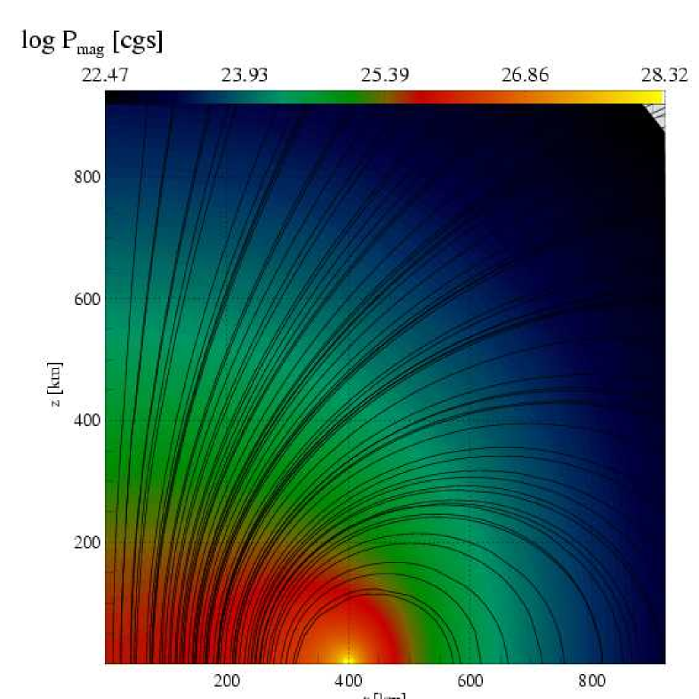
Figure 1: The initial magnetic field configuration of the models of series AaBbGg-D3M13. Besides the field lines the distribution of the magnetic pressure (color coded) is displayed. $P_{\mathrm{mag}}$ is largest near the center of the field generating current loop located at a radius of $r_{\mathrm{mag}}^{D3}=400\ \mathrm{km}$ in the equatorial plane, and drops rapidly with increasing radius for $r>r_{\mathrm{mag}}^{D3}$.

2.4 Gravitational-wave emission

During collapse, bounce, and explosion the rapid infall of matter and in particular its more or less abrupt slowdown give rise to strong variations of the matter–density quadrupole moment of any aspheric core. This causes the emission of gravitational radiation.

We calculate the gravitational wave amplitude of the core using the quadrupole formula in spherical coordinates, and applying the extension of the formulation of Mönchmeyer et al. (1991, MSMK, hereafter) to the MHD case due to Kotake et al. (2004b). Our treatment includes the hydrodynamic, gravitational, and magnetic forces acting on the fluid. We calculate the quadrupole amplitude $A^{\mathrm{E}2}_{20}$ according to the formula (see Appendix C):

$$A^{\mathrm{E}2}_{20} = \frac{G}{c^{4}}\frac{32\pi^{\frac{3}{2}}}{\sqrt{15}}\int_{0}^{1}\mathrm{d}z\int_{0}^{\infty}\mathrm{d}\frac{r^{3}}{3}$$ (15)

$$\left[f_{rr}(3z^{2}-1)+f_{\theta\theta}(2-3z^{2})-f_{\phi\phi}-6f_{r\theta}z\sqrt{1-z^{2}}-\right.$$

$$\left.-r\partial_{r}\Phi(3z^{2}-1)+3\partial_{\theta}\Phi z\sqrt{1-z^{2}}\right],$$

where the components of $f_{ij}$ are given by

$$f_{ij}=\rho v_{i}v_{j}-b_{i}b_{j}.$$ (16)

In the following, we will refer to the various parts of the total amplitude as follows: $A^{\mathrm{E}2}_{20;v_{i}v_{j}}$, $A^{\mathrm{E}2}_{20;b_{i}b_{j}}$, and $A^{\mathrm{E}2}_{20;\mathrm{G}_{i}}$ denote the contributions of the terms involving $v_{i}v_{j}$, $b_{i}b_{j}$, and $\partial_{i}\Phi$ in Eq. 15, respectively. Furthermore $A^{\mathrm{E}2}_{20;\mathrm{hyd}}$, $A^{\mathrm{E}2}_{20;\mathrm{mag}}$, and $A^{\mathrm{E}2}_{20;\mathrm{grav}}$ are the sums over all components of $A^{\mathrm{E}2}_{20;v_{i}v_{j}}$, $A^{\mathrm{E}2}_{20;b_{i}b_{j}}$, and $A^{\mathrm{E}2}_{20;\mathrm{G}_{i}}$, respectively.

The radiative quadrupole moment $M^{\mathrm{E}2}_{20}$ (Eq. 43) is a measure of the asphericity of the core’s density distribution. It is positive for a very prolate core, and negative in the limit of very oblate cores. Its first time derivative $N^{\mathrm{E}2}_{20}$ (Eq. 44) measures the asphericity of the mass–flux and the momentum distribution of the core, and its second time derivative, the quadrupole amplitude $A^{\mathrm{E}2}_{20}$, is a measure of the asphericity of the forces acting on the fluid. As a rule of thumb, a prolate mass–flux or a prolate momentum distribution (e.g. a bipolar jet–like outflow along the rotational axis) gives rise to a positive value of $N^{\mathrm{E}2}_{20}$. Forces that act on the core in a way to make it more oblate, such as the centrifugal force that has its manifestation in the $A^{\mathrm{E}2}_{20;v_{\phi}v_{\phi}}$ part of the amplitude, will give rise to a negative contribution to the total amplitude (negative sign of the $A^{\mathrm{E}2}_{20;v_{\phi}v_{\phi}}$ term in Eq. 15).

The different signs of the hydrodynamic and the magnetic contributions to the amplitude (Eq. 16) resulting from the different signs of the hydrodynamic (Reynolds) and the magnetic (Maxwell) stresses in the MHD flux terms, will – for suited topologies of field and flow – lead to a more or less prominent phase shift between the hydrodynamic and the magnetic amplitude. If the gravitational wave amplitude $A^{\mathrm{E}2}_{20;\mathrm{G}_{i}}$ is in phase with the hydrodynamic amplitude $A^{\mathrm{E}2}_{20;\mathrm{hyd}}$ (which holds well for many models, in particular for those with relatively long oscillation periods; see Sect. 4), the magnetic amplitude $A^{\mathrm{E}2}_{20;\mathrm{mag}}$ may be phase shifted with respect to $A^{\mathrm{E}2}_{20;\mathrm{hyd}}+A^{\mathrm{E}2}_{20;\mathrm{G}_{i}}$. Such a phase shift was observed by Yamada & Sawai (2004).

3 Numerical method

The MHD equations are integrated using a newly developed Eulerian, finite volume code based on the algorithm devised by Pen et al. (2003). This code employs the relaxing TVD method of Jin & Xin (1995) for the solution of the advection equations and the constraint–transport formulation of Evans & Hawley (1988) to deal with the divergence constraint of the magnetic field.

We have rewritten the original code of Pen et al. in order to adjust for the simulations of stellar core collapse. This included the transformation of the equations from Cartesian to spherical coordinates, the calculation of the gravitational potential, the implementation of the gravitational source terms in the momentum and energy equations, and the implementation of an approximate equation of state for iron core matter. The integration of the fluid equations and of the induction equation is based on a second-order (piecewise–linear) relaxing TVD method. For a short summary of this method see Appendix A. For the time evolution we use an operator–split approach based on a method of lines (LeVeque, 1992).

The simulations were performed on a grid of 380 logarithmically spaced radial zones up to $R_{\star}\ \mathrm{km}$, where $R_{\star}\sim 1700...2000\ \mathrm{km}$ is the radius of the initial stellar model. The central resolution was $(\Delta_{r})_{\mathrm{c}}\approx 300\ \mathrm{m}$. The angular grid consisted of 60 equidistant zones in the domain $0\leq\theta\leq\frac{\pi}{2}$. This grid resolution has been chosen after obtaining converged results when running several models at different resolutions. The numerical convergence of our simulations is demonstrated in the Appendix (Sect. B).

The stellar models used by us (polytropes) are quite compact configurations of matter characterized by a sharp transition from a high density interior to a low density surface layer. Note that this feature is also seen in sophisticated stellar evolution calculations, which predict a steep density gradient at the outer edge of the iron core. In rotating models the transition layer is aspherical and must completely be contained within the spherical boundary of the numerical grid, i.e. its numerical treatment requires special care. Grid zones outside the core are filled with an ”atmosphere” fluid of some prescribed density $\rho_{\mathrm{atmo}}$ at rest. During collapse the infall of matter creates a region near the edge of the core where the density might become so low that numerical problems arise. To overcome these difficulties, we follow the approach of DFM1 and set the hydrodynamic variables $\rho,\@vec{v},e$ equal to some prescribed values $\rho_{\mathrm{atmo}},\@vec{0},e_{\mathrm{atmo}}$ in all zones where the fluid density falls short of a given threshold $\rho_{\mathrm{cut}}$. In this way the atmosphere can adjust to the (non–spherical) varying shape of the star. We used $\rho_{\mathrm{cut}}=10^{5}\ \mathrm{cm\,s}^{-1}$, and set $\rho_{\mathrm{atmo}}=10^{3}\ \mathrm{cm\,s}^{-1}$. From the atmospheric density and velocity one can calculate the energy density assuming zero thermal energy.

The evolution of the magnetic field is turned off for zones marked as atmosphere, i.e. $\@vec{b}$ remains constant in the atmosphere consistent with the assumed zero velocity of the atmosphere gas.

4 Results

The results of our simulations show that magneto–rotational collapse can be categorized in essence into two limiting cases depending on the strength of the initial magnetic field. If the initial magnetic field is weak, its influence on the dynamics and the gravitational wave emission is negligible during the time scales of our simulations (see Sect. 4.1). The results of the hydrodynamic simulations of ZM and DFM apply in this case without any modification. On the other hand, and not unexpectedly, initially strongly magnetized cores evolve quite differently, as will be discussed in Sect. 4.2. Note that since the MRI acts independently of the strength of the initial magnetic field, the distinction between dynamically negligible and dynamically important fields may be an artificial one resulting from our inability to simulate the MRI for magnetic fields below a certain threshold (see Sect. 4.3). Hence, also initially weak magnetic fields may cause similar dynamical effects as strong ones. The dependence of our results on the initial magnetic field configuration will be discussed in Sect. 4.4, and further information about the temporal evolution of all models is provided in appendix D.

4.1 Weak initial fields

4.1.1 GW signal and dynamics

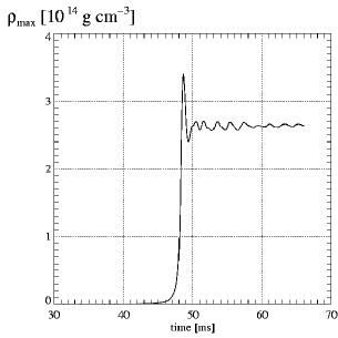
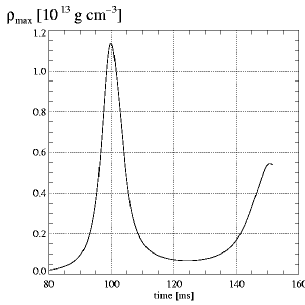
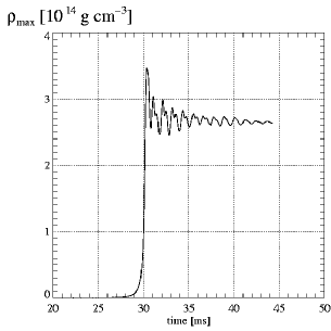
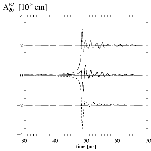
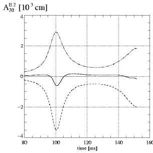
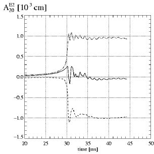
Figure 2: The evolution of the maximum density (top panels) and the GW amplitude (bottom panels) of three weak–field models: the standard type-I model A1B3G3-D3M10 (left panels), the type-II model A2B4G1-D3M10 (middle panels), and the type-III model A3B3G5-D3M10 (right panels). The bottom panels show the total GW amplitude $A^{\mathrm{E}2}_{20}$ (solid lines) together with the partial amplitudes $A^{\mathrm{E}2}_{20;\mathrm{hyd}}$ (dashed lines), $A^{\mathrm{E}2}_{20;\mathrm{mag}}$ (dash-dotted lines; here almost zero), and $A^{\mathrm{E}2}_{20;\mathrm{grav}}$ (dash-dot-dot-dot line).

The gravitational wave signals of initially weakly magnetized cores do not differ from those obtained by MM, ZM and DFM for the corresponding non–magnetized initial models, because the magnetic fields never become dynamically important during the simulations. Consequently, both the magnetic force contribution to the GW amplitude (see Sect. 2.4) and the back–reaction of the magnetic field on the flow are negligible. This ”weak–field” behavior holds for most models with initial fields of $\la 10^{11}\ \mathrm{G}$. However, in some models bouncing at relative low central density due to centrifugally forces (e.g. models A4B5G5-D3M12 and A2B4G1-D3M12) even a field of $10^{12}\ \mathrm{G}$ does not affect the evolution of the core significantly. We note that these numbers may change when the field amplification by the MRI, which works independently of the seed field strength, is properly simulated (see Sect. 4.3).

Three types of GW signals are distinguished by MM and ZM which they call type-I, type-II, and type-III, respectively. The evolution of three representative weak–field models that emit these different signal types is illustrated in Fig. 2. Although the GW signals are very similar to those of the corresponding non–magnetized cores of ZM, we will discuss them and the underlying dynamics here in some detail for reason of comparison with the GW signals of strongly magnetized cores (see Sect. 4.2).

In the case of a type-I (or standard–type) GW signal (model A1B3G3-D3M10; Fig. 2, left panels), the core bounces due to the stiffening of the nuclear EOS at supra–nuclear densities. Pressure waves crossing the inner core stop the infall and lead to the formation of an outward moving shock wave. Hence, the typical time scale is roughly given by the sound crossing time of the inner core at bounce ($\sim 1\,$ms). After bounce the core exhibits damped oscillations on roughly the same time scale. During collapse, the GW amplitude is increasingly positive due to the gravity contribution $A^{\mathrm{E}2}_{20;\mathrm{grav}}>0$ which dominates the hydrodynamic one $A^{\mathrm{E}2}_{20;\mathrm{hyd}}<0$. At bounce the GW amplitude decreases strongly assuming large negative values, because the modulus of the centrifugal contribution $A^{\mathrm{E}2}_{20;v_{\phi}v_{\phi}}$ becomes very large when the rotational energy approaches its maximum. The oscillations of the core produce the oscillations of $A^{\mathrm{E}2}_{20;\mathrm{grav}}$ and hence of the total GW amplitude on the same time scale. As the shock wave is almost spherical (except for initially very rapidly rotating cores), the post–bounce GW amplitude is predominantly produced by the central core with only a modest contribution of the outer layers. The hydrodynamic contribution $A^{\mathrm{E}2}_{20;\mathrm{hyd}}$ is dominated by $A^{\mathrm{E}2}_{20;v_{\phi}v_{\phi}}$.

A type-II signal (model A2B4G1-D3M10; Fig. 2, middle panels) is emitted, if, for an initially sufficiently fast rotation and a sufficiently large degree of differential rotation, the core suffers a bounce due to centrifugal forces before nuclear density is reached. After bounce the core exhibits several large amplitude oscillations, which are considerably less damped than in the case of a pressure dominated bounce. The oscillations are reflected in the GW signal: each time the density reaches a maximum the GW amplitude becomes strongly negative, while being positive otherwise. The negative GW amplitude again results from the enhanced rotational energy during this collapse phase when the inner core also becomes strongly oblate. The contribution of the centrifugal-force amplitude $A^{\mathrm{E}2}_{20;v_{\phi}v_{\phi}}$ to the hydrodynamic one $A^{\mathrm{E}2}_{20;\mathrm{hyd}}$ is negligible. Since much of the dynamics happens at relatively large radii, the GW signal is produced by the whole core. The contribution of the central core is typically negative because of its rotationally flattened, oblate shape, whereas the outer layers contribute to the overall amplitude with a positive signal due to the prolate shape of the outward propagating shock wave.

The signals of type III (model A3B3G5-D3M10; Fig. 2, right panels) that are emitted by cores collapsing very rapidly due to a very soft sub–nuclear EOS are characterized by the lack of a strongly negative GW amplitude at bounce. This results from the only modest rise of the rotational energy at bounce implying a relatively small centrifugal contribution to the GW signal $A^{\mathrm{E}2}_{20;v_{\phi}v_{\phi}}$, and from the relatively large positive contribution of the still collapsing layers outside to the shock wave. Past bounce the signal exhibits rapid (on the hydrodynamic time scale $t_{\mathrm{hyd}}\approx 1,$ms) oscillations like the maximum density. The contributions from the outer layers of the core are also responsible that the signal then remains positive for an extended period of time (i.e. several oscillation periods) during which the amplitude gradually decreases.

4.1.2 Field amplification

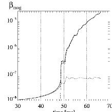
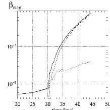
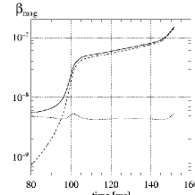
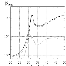
Figure 3: The evolution of the magnetic energy parameters $\beta_{\mathrm{mag}}$ (total energy, solid line), $\beta_{\phi}$ (toroidal field energy, dashed line), and $\beta_{\mathrm{mag}}-\beta_{\phi}$ (poloidal field energy, dotted line) of models A1B3G3-D3M10 (upper left panel), A3B3G5-D3M10 (upper right panel), A2B4G1-D3M10 (lower left panel), and A4B5G5-D3M10 (lower right panel), respectively. Note that in the upper left panel $\beta_{\mathrm{mag}}\approx\beta_{\phi}$ and, thus, both lines are almost indistinguishable.

The evolution of the magnetic energy is illustrated for four selected models in Fig. 3 showing the ratio of the field energy and the gravitational energy for the total ($\beta_{\mathrm{mag}}$), toroidal ($\beta_{\phi}$), and poloidal ($\beta_{\mathrm{mag}}-\beta_{\phi}$) magnetic field, respectively. Both the total and the toroidal magnetic energies rise sharply at bounce by a factor of $10^{2}$ to $10^{3}$. The magnetic energy is mostly stored in form of the toroidal magnetic field $B_{\phi}$, which is created from the poloidal component by the action of differential rotation. The amplification process extends beyond the end of our simulations.

As our study is restricted to axisymmetric simulations, the main field amplification mechanism is the conversion of rotational into magnetic energy via the $\Omega$–dynamo. Axisymmetry suppresses most of the instabilities of the (toroidal) field that are necessary to close the dynamo loop of a full $\alpha-\Omega$ dynamo, where a poloidal field is converted into a toroidal one and amplified by differential rotation, and then converted back into a poloidal field by some instability of the toroidal field (Spruit, 1999, 2002).

Before we discuss the properties of some models in greater detail, we summarize a few general trends:

• The larger the initial rotational energy (for a given degree of differential rotation and a given EOS), the larger is the rate of field amplification.

• The higher the degree of differential rotation (for a given $\beta_{\mathrm{rot}}$), the larger is the rate of field amplification.

• Among a series of models with the same initial configuration, the magnetic field is amplified more efficiently for models whose EOS has a larger sub–nuclear adiabatic index $\Gamma_{1}$ and do not suffer a centrifugal bounce. The time scale for the amplification of the magnetic field is set by the rotation period of the core.

• The collapse of models with a relatively stiff sub–nuclear EOS (AaBbG1-DdMm) leads to a very extended post–bounce core having a rotational frequency much less than that of a corresponding type-I model even though the rotational energy and $\beta_{\mathrm{rot}}$ may be larger in the former model. Thus, the field is amplified more slowly in models suffering a sub–nuclear bounce due to centrifugal forces, and their cores experience several phases of expansion during which they slow down. This leads to a significantly less efficient amplification or even a weakening of the magnetic field. We thus find that type-I models are most efficient in terms of magnetic field amplification.

• Due to the efficient field amplification most of our weak–field models reach magnetic field strengths of the order of $10^{13}\mathrm{G}$ to $10^{15}\mathrm{G}$ within a few tens of milliseconds after core bounce. This is in the range of field strengths observed in magnetars. From the definition of $\beta_{\mathrm{mag}}$ follows, that

  $$\beta_{\mathrm{mag}}\sim\frac{\frac{4\pi}{3}b^{2}/2\ R^{4}}{GM^{2}},$$ (17)

  where $b$ is a typical value of the field within the core, and $R$ and $M$ are its mass and radius, respectively. Thus, a typical post–bounce field corresponds to a magnetic energy parameter of

  $$\beta_{\mathrm{mag}}\sim 0.05\ \%\left(\frac{b}{10^{15}\ \mathrm{G}}\right)^{2}\left(\frac{R}{20\ \mathrm{km}}\right)^{4}\left(\frac{M}{0.5\ M_{\sun}}\right)^{-2}.$$ (18)

The maximum energy that can go into the magnetic field is limited by the energy that is contained in the differential rotation of the core. None of our weak–field cores is evolved long enough for the field to reach saturation strength. However, examining the field amplification process for models with strong ($\ga 10^{12}\mathrm{G}$) initial fields, which reach dynamically important values not too early, we conclude that efficient field amplification ceases when the magnetic energy of the collapsed core approaches a significant fraction of its rotational energy, i.e. some ten percent. As all of our cores initially have similar rotational energies ($\beta_{\mathrm{rot}}$ about a few percent), we expect them to reach (surface) field strengths of the same order if there is sufficient time for amplification. From our models with initially stronger fields we can estimate the saturation field strengths to be of the order of $b\ga 10^{15}\ \mathrm{G}$. Using the estimate for $\beta_{\mathrm{mag}}$ given above (18), these fields correspond to $\beta_{\mathrm{mag}}\sim(0.05...5)\,\%$. Such values we have found in our simulations. The magnetic field in most post–bounce cores is strongly concentrated in the inner core, reflecting the density structure. Thus, for usual standard–type cores, the field is strongest a few kilometres from the center, and drops rapidly towards larger radii. When a strong shear layer is present at the surface of the inner core, the field may also be strongest there. This is the case for many of the weak-field cores, but does not necessarily hold for the strong-field ones. In the latter case, the simulations tend to give values of $\beta_{\mathrm{mag}}$ in excess of the previous estimate.

The field amplification via the $\Omega$–dynamo is most efficient, if the poloidal field component is large compared to the toroidal one. A characteristic growth time for the generation of $b_{\phi}$ from a radial component $b_{\varpi}$ is given by (Meier et al., 1976)

$$\tau_{\Omega}=\frac{b_{\phi}}{b_{\varpi}\varpi\partial_{\varpi}\Omega}\,.$$ (19)

In our models the poloidal component does not grow after bounce (apart from the effects of compression and expansion during the large–scale oscillations of type-II models) unless there is an instability (Fig. 3; Sect. 4.3).

The rate of field amplification is similar for the fast collapsing cores A1B3G5-D3M10, A2B4G5-D3M10 and A3B3G5-D3M10, which have a soft sub–nuclear EOS and which do not suffer a centrifugal bounce. A slightly more efficient amplification is observed for the initially more differentially and faster rotating cores A2B4G5-D3M10 and A3B3G5-D3M10 than for the initially rigidly rotating model A1B3G5-D3M10. An even faster amplification is observed for the slower collapsing model A1B3G3-D3M10, where 10 ms after bounce $\beta_{\mathrm{mag}}=8\cdot 10^{-5}$ compared to $\beta_{\mathrm{mag}}=8\cdot 10^{-6}$ for model A3B3G5-D3M10 (Fig. 3, upper two panels). This reflects the different infall profiles of the cores whereby the regions of strongest magnetic field (initially around and interior to the field generating current loop at $r_{\mathrm{mag}}=400\ \mathrm{km}$) are swept along to different positions in the core. In case of the model A1B3G3-D3M10 this region is much closer ($r\approx 40\ \mathrm{km}$) to the center at the time of bounce than for model A3B3G5-D3M10, where it is located at $r\approx 120\ \mathrm{km}$. Therefore, the fraction of the magnetic field that is available in the regions where the $\Omega$–dynamo acts most efficiently is larger for the former model, i.e. the field amplification can proceed more efficiently.

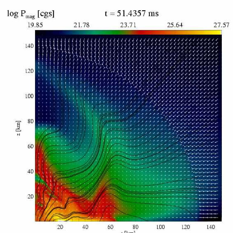
Figure 4: Magnetic pressure (color shaded), velocity field (arrows), and magnetic field lines of model A1B3G3-D3M10 at $t=51.44\ \mathrm{ms}$.

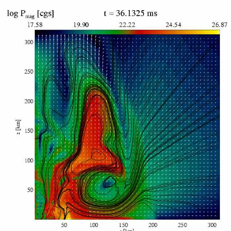
Figure 5: Same as Fig. 5, but for model A4B5G5-D3M10 at $t=36.13\ \mathrm{ms}$.

During collapse and to an even larger extent during and after core bounce the magnetic field configuration of model A1B3G3-D3M10 is considerably distorted. The field lines initially surrounding the off–center current loop (Fig. 1) are pulled towards the center. Apart from an overall compression the field geometry remains basically the same as in the initial model. A complex pattern of “filamentary” regions of high and low magnetic fields develops as the field lines get entangled by the fluid flow around and after bounce. No simple classification of the magnetic field as a dipole, quadrupole, etc., is possible. In the subsequent evolution the tangled fields follow the outward propagating shock front which is almost spherically symmetric in this initially rigidly rotating model (Fig. 4).

Multiple–bounce models that experience several phases of collapse and expansion exhibit a similar evolution of the magnetic field. During a contraction phase angular momentum conservation yields a more efficient amplification of the magnetic field energy, whereas $\beta_{\mathrm{mag}}$ grows much slower in an expansion phase. This is the case for model A2B4G1-D3M10 (Fig. 3, lower left panel). The magnetic energy parameter $\beta_{\mathrm{mag}}$ rises by a factor $\approx 3$ during $10\,$ms around core bounce ($t_{\mathrm{b}}\approx 100\ \mathrm{ms}$), but then requires $40\,$ms to amplify the field by another factor of $\approx 1.6$. The amplification rate increases again strongly during the subsequent contraction phase. For model A4B5G5-D3M10, the amplification factor during core bounce is about $20$, but later the field energy gets greatly reduced ($\beta_{\mathrm{mag}}$ drops by a factor $\approx 3.5$) during the extremely violent expansion that follows the bounce in this model (Fig. 3, lower right panel; the evolution of the maximum density is shown in Fig. 19). Afterwards, differential rotation again starts to increase the magnetic field, but on a longer time scale.

Model A4B5G5-D3M10 possesses a torus shaped initial density distribution, and maintains it throughout the entire evolution. The field structure of this model tends to become very complex during the evolution. In the final model, at $t=36.13\ \mathrm{ms}$, the field exhibits both sheet–like regions of strong fields ($\approx 100\ \mathrm{km}$ off the axis), and also toroidal (at $r\approx 120\,\ \mathrm{km}$, $z\approx 60\ \mathrm{km}$) and cylindrical (e.g.  $\approx 50\ \mathrm{km}$ off the axis) weak–field regions (Fig. 5).

4.2 The strong field case

For initially strong magnetic fields the collapse shows significant deviations from the purely hydrodynamic case. The most striking new feature is the braking of the rotation of the core by magnetic stresses. The initially strongest fields are amplified by differential rotation during collapse to such a level that they can cause considerable braking, whereas initial fields of the order of $10^{12}\ \mathrm{G}$ or less require the action of an MRI–like instability to reach a level sufficient for significant angular momentum transport on the collapse time scale. In the following we will first discuss the former class of models divided into models bouncing due to pressure forces (Sect. 4.2.1) or centrifugal forces (Sect. 4.2.2), and later address the issue of the MRI in Sect. 4.3.

4.2.1 Models bouncing due to pressure forces

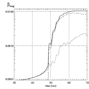
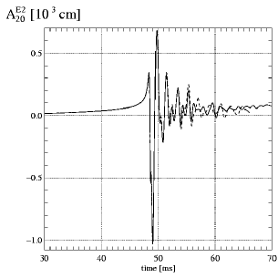
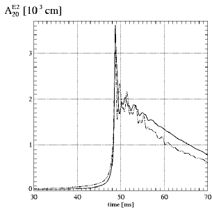
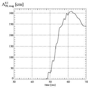
Figure 6: The dynamics and the GW signal of model A1B3G3-D3M12. The upper left and middle panels provide a comparison of the evolution of the rotational energy parameter $\beta_{\mathrm{rot}}$ and the maximum density of this model (solid lines) with those of model A1B3G3-D3M10 (dashed lines). The upper right panel displays the evolution of $\beta_{\mathrm{mag}}$ (solid line), $\beta_{\phi}$ (dashed line), and $\beta_{\mathrm{mag}}-\beta_{\phi}$ (dotted line), respectively. The GW signal is shown in the lower panels: total amplitude (solid line, left; the dashed line gives the total amplitude of model A1B3G3-D3M10), $-A^{\mathrm{E}2}_{20;\mathrm{hyd}}$ (solid line, middle), $A^{\mathrm{E}2}_{20;\mathrm{grav}}$ (dashed line, middle), and $A^{\mathrm{E}2}_{20;\mathrm{mag}}$ (right). The corresponding variables of model A1B3G3-D3M10 are shown in Fig. 2.

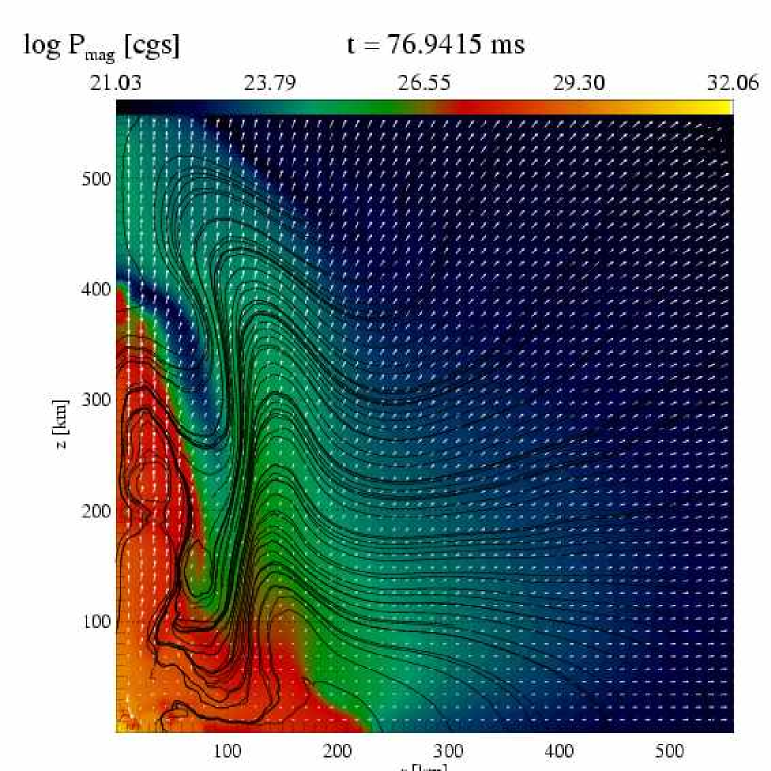
Figure 7: Snapshot of the inner regions of model A1B3G3-D3M12 at $t=76.94\ \mathrm{ms}$ showing the magnetic pressure (color shaded), the bipolar flow field (vectors), and the magnetic field lines, respectively.

As in the case of weak–field models, the poloidal field energy of a single bounce models such as A1B3G3-D3M12 is approximately constant during the early post–bounce evolution, but it is strongly amplified afterwards by MRI–like modes in the core which efficiently remove angular momentum from the inner core and decrease its rotational energy. The evolution of the rotational energy hence shows a clear deviation from that of a weak–field model (Fig. 6), which however should not be the case, as the MRI does not depend on the seed field. We will explain in Sect. 4.3 why this different behavior arises.

The loss of rotational support also affects the density structure. The core of model A1B3G3-D3M12 is slightly less rotationally flattened than the core of a non–magnetized model such as A1B3G3-D3M10. The shock that forms at bounce, when the models hardly differ, is unaffected by the different evolution of the central region, whereas matter in the central region experiences an additional acceleration due to the presence of the strong magnetic field. The decrease of the rotation rate, and also of the degree of differential rotation in the strong–field case limits the amplification of the toroidal field component by wrapping of field lines (Fig. 6, upper right panel), and the total magnetic energy has a significant poloidal contribution. At $t\approx 70\ \mathrm{ms}$, the ratio of toroidal and total magnetic energy has dropped to a value of about $80\,\%$. The poloidal component grows a little during the post–bounce evolution by the action of meridional motions in the core. When the magnetic field becomes dynamically important, magnetic energy is used to accelerate the fluid, which puts an end to the phase of efficient field amplification. During the late stages of evolution, the total field energy remains approximately constant. Its final value corresponds to $\beta_{\mathrm{mag}}\approx 1\,\%$. The field structure of model A1B3G3-D3M12 differs from that of the weak–field core A1B3G3-D3M10 in the central parts of the core at late times due to the MRI modes (that could not be resolved for the weaker field; see Sect. 4.3), but farther away from the center the fields have a similar topology.

Around the time of bounce the GW signal of model A1B3G3-D3M12 is very similar to the one of the less magnetized core A1B3G3-D3M10, and also the contributions of the individual parts of the total signal are comparable (Fig. 6, lower panels). In the post–bounce evolution, both the hydrodynamic and the gravitational part of the amplitude start to decrease in magnitude, as the rotationally induced asphericity of the core decreases along with the extraction of rotational energy. The magnetic amplitude increases strongly as magnetic forces act on the core decreasing its rotation. The oscillations of the core are still imprinted on the post–bounce GW amplitude, but their impact on the signal decreases with time. In the long run, the amplitude assumes positive values and varies relatively little. Dynamically, this phase is characterized by the emergence of a weak outflow along the polar axis far behind the shock wave created at core bounce. This outflow is predominantly driven by magnetic forces (Fig. 7). The positive long–term GW amplitude is mainly due to the $A^{\mathrm{E}2}_{20;v_{r}v_{r}}$ term which is large inside the outflow, whereas the inner parts of the model and the almost spherical shock wave contribute little to the total signal. Despite the differences in the post–bounce GW amplitude contributions of the two models A1B3G3-D3M10 and A1B3G3-D3M12 their total signals are quite similar, i.e. distinguishing the two models observationally would be very difficult.

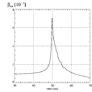
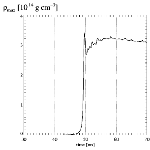
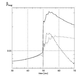
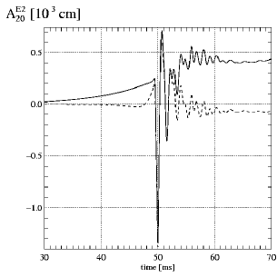
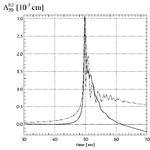
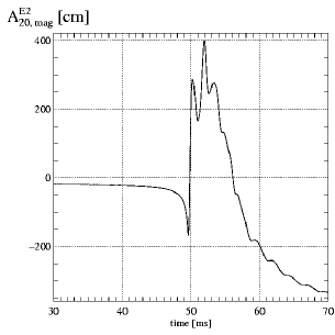
Figure 8: The dynamical evolution and the GW signal of model A1B3G3-D3M13. The upper panels display the temporal evolution of the rotational energy parameter $\beta_{\mathrm{rot}}$ (left), the maximum density $\rho_{\mathrm{max}}$ (middle), and the magnetic energy parameters (right; $\beta_{\mathrm{mag}}$ (solid line), $\beta_{\phi}$ (dashed line), and $\beta_{\mathrm{mag}}-\beta{\phi}$ (dotted line)), respectively. The GW signal of the model is shown in the lower panels: total amplitude (solid line, left; the dashed line gives the contribution of the layers with $r\leq 59.4\,$km), $-A^{\mathrm{E}2}_{20;\mathrm{hyd}}$ (solid line, middle), $A^{\mathrm{E}2}_{20;\mathrm{grav}}$ (dashed line, middle), and $A^{\mathrm{E}2}_{20;\mathrm{mag}}$ (right).

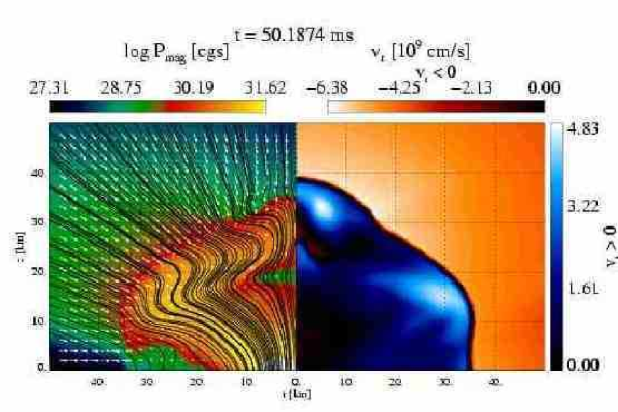
Figure 9: Snapshot of model A1B3G3-D3M13 at $t=50.19\ \mathrm{ms}$, when the maximum density reaches the first post-bounce minimum. In the left panel the flow field (vectors) and the magnetic field (field lines) are displayed together with the magnetic pressure (color–coded). The right panel shows the color–coded velocities of in-flowing (i.e.  $v_{r}>0$) and out-flowing matter (i.e.  $v_{r}<0$), respectively.

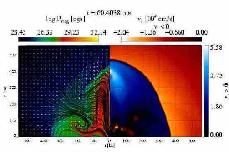
Figure 10: Same as Fig. 9, but at $t=60.40\ \mathrm{ms}$. Note that the length scales are changed compared to Fig. 9.

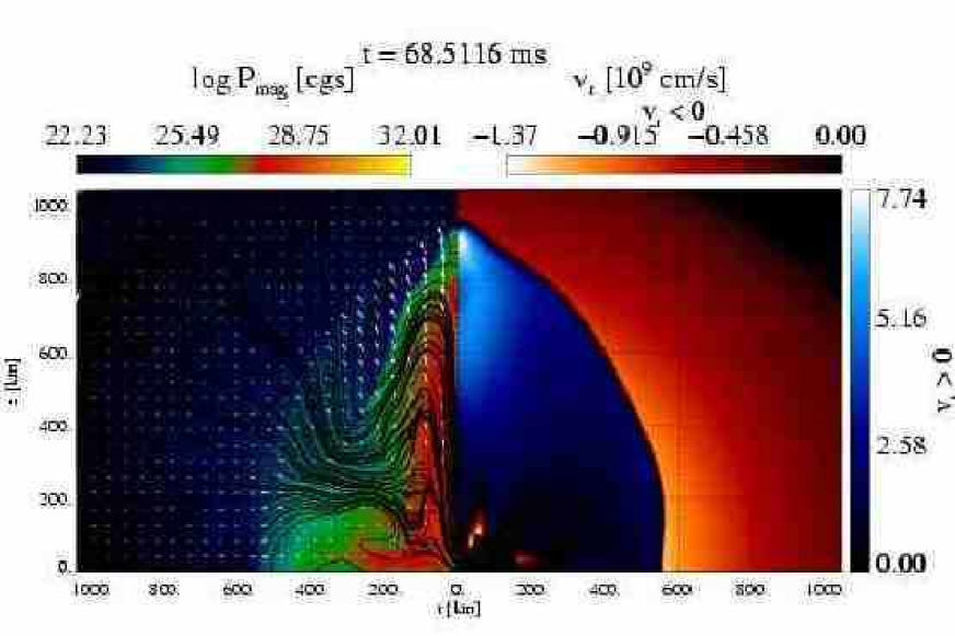
Figure 11: Same as Fig. 9, but at $t=68.51\ \mathrm{ms}$. Note that the length scales of the plot are changed compared to Figs. 9 and 10.

Similar features as those observed in the case of model A1B3G3-D3M12 (Fig. 6) are present in the evolution of the stronger magnetized model A1B3G3-D3M13 (Fig. 8), but they are much more prominent. Unlike all previously discussed models, this core shows significant deviations from the purely hydrodynamic case already during collapse. For model A1B3G3-D3M13 the core bounce is delayed by $\approx 1\ \mathrm{ms}$ compared to the weaker magnetized models A1B3G3-D3M10…12. The rotational energy reaches a maximum value of $\beta_{\mathrm{rot}}^{\mathrm{max}}\approx 7\,\%$ near bounce, which is lower than in the less magnetized models ($\beta_{\mathrm{rot}}^{\mathrm{max}}\approx 8\,\%$). Within the next $\approx 6\ \mathrm{ms}$ the core looses $\approx 80\,\%$ of the rotational energy it had acquired at bounce. Subsequently, the rate of energy loss decreases, and the core contracts (Fig. 8). Its maximum density rises from $\rho_{\mathrm{max}}=2.7\cdot 10^{14}\ \mathrm{cm\,s}^{-1}$ in the first post–bounce density minimum to $\rho_{\mathrm{max}}=3.2\cdot 10^{14}\ \mathrm{cm\,s}^{-1}$ at $t=58\ \mathrm{ms}$ before it starts to decreases by a small amount again. The process of magnetic braking prevents a further amplification of the field, and it prevents the transformation of poloidal into toroidal magnetic field. The ratio $\beta_{\phi}/\beta_{\mathrm{mag}}$ does not approach unity, as in case of the models with weaker initial fields, but it remains below $\approx 60\,\%$ decreasing slowly later. At $t\approx 71\mathrm{ms}$, when we stopped the computations, the value of $\beta_{\mathrm{mag}}$ had dropped to $\beta_{\mathrm{mag}}\approx 2.05\,\%$, and we expect it to eventually decrease to a value of $\sim 1\,\%$.

In model A1B3G3-D3M12 the immediate post–bounce core is very similar to the corresponding non–magnetic one as the magnetic field is not sufficiently strong to change the dynamics unless an MRI–like instability sets in. This is different from the more strongly magnetized model A1B3G3-D3M13, where without the MRI the combined amplification due to contraction and differential rotation is sufficient to cause the braking effect. This is generally true for all of our models: very strong initial fields ($>10^{12}\ \mathrm{G}$) do not need amplification by an instability to brake the core, whereas weaker ones heavily depend on it.

After bounce, the shock wave develops a non–spherical, bulb–like shape , and the twisted field lines give rise to a highly magnetized post–shock fluid that pushes the shock near the equatorial plane around $\theta\approx 70\degr$ (Fig. 9). Near the axis, the immediate post-shock matter is only weakly magnetized, the ratio of gas pressure and magnetic pressure being largest at a significantly smaller radius ($r_{\mathrm{max,mag}}\approx 27\ \mathrm{km}$) than the shock position ($r_{\mathrm{shock}}\approx 40\ \mathrm{km}$). The shock maintains its bulb–like shape also during the secondary contraction phase that goes along with the extraction of rotational energy, and fast outflow both at high and low latitudes. At later times ($t=60.40\ \mathrm{ms}$, Fig. 10), the fluid pattern has changed. The formerly important outflow near the equator stalls, and the shock surface becomes more elongated. The near–axis outflow velocity has further increased, its maximum value being $v_{r}^{\mathrm{max}}=0.19c$ in the strongly magnetized region well behind the shock ($r_{\rm{maxmag}}=270\ \mathrm{km}<r_{\mathrm{shock}}=330\ \mathrm{km}$). In the outflow along the rotational axis, a cylindrical shell of very low pressure gas can be identified (at $\theta\approx 10\degr$ in Fig. 10). The structure of the magnetic field is dominated by two extended highly magnetized regions, one located near the equator at $(r\la 200\ \mathrm{km}$, $\theta\approx 80\degr$), and a cylindrical one oriented along the rotational axis having a width of $\approx 100\,$km (left panel of Fig. 10). At an even later epoch, $t=68.51\ \mathrm{ms}$ (Fig. 11), only little has changed near the equatorial plane, however at the axis the highly magnetic gas is about to catch up with the shock wave, which is now significantly prolate with an axis ratio of about $3:2$. The outflow has accelerated further ($v_{r}=8\cdot 10^{9}\ \mathrm{cm\,s}^{-1}\sim c/4$), the maximum velocity corresponding to the highly magnetized regions behind the shock at $r=870\ \mathrm{km}$. Hence, we see the formation of a jet–like outflow from the core.

In its very interior the core is rotating slower than its non–magnetic variant at late times. Furthermore, it has developed a roughly toroidal region of relatively slow and highly rigid counter–rotation. This region grows from a layer at $r\approx 10\ \mathrm{km}$, i.e. near the edge of the inner core, which experiences sufficiently strong magnetic stresses to reverse its direction of rotation. Interior to the retrograde rotating region the angular velocity decreases with time.

Assuming that the total energy density of a fluid element, $e_{\mathrm{tot}}=\varepsilon+\frac{1}{2}\rho\@vec{v}^{2}+\frac{1}{2}\@vec{b}^{2}-\rho\cdot\Phi$, is converted entirely into kinetic energy $\frac{1}{2}\rho v_{\infty}^{2}$, terminal outflow velocities $v_{\infty}$ of up to $1.85\cdot 10^{10}\ \mathrm{cm\,s}^{-1}$ are observed for model A1B3G3-D3M13 at late times, particularly in the bipolar outflow along the rotation axis (Fig. 11). The large velocities stretch our non–relativistic MHD approach, and imply that a realistic simulation of the late evolution of the outflow will require relativistic MHD.

The GW amplitude of model A1B3G3-D3M13 (Fig. 8, lower panels) is enhanced by about $10\,\%$ at core bounce. After bounce, ringing on the dynamical time scale of the core the average amplitude shifts to positive values. The amplitudes and frequencies of the oscillations are hardly affected by the overall shift of the average amplitude to positive values implying a different origin of the oscillations and the overall shift. A few milliseconds after bounce $A^{\mathrm{E}2}_{20}$ grows to $\sim 400\ \mathrm{cm}$, and the rapid variations of the signal cease. The hydrodynamic and gravitational contributions to the total amplitude are greatly reduced in magnitude. The inner core has lost a large amount of its rotational energy and is of almost spherical shape. Its contribution to the total signal amplitude is hence relatively small for epochs well after bounce.

Figure 12: The hydrodynamic plus gravitational parts of the GW amplitude of model A1B3G3-D3M13 at $t=68.5\ \mathrm{ms}$. Positive contributions to the integrand in the formula for the hydrodynamic plus gravitational amplitude are displayed by colors. The bipolar outflow shows up in the large positive parts near the axis.

While the hydrodynamic amplitude produced by the innermost layers of the core is very small, the gravitational and magnetic contributions reach quite large values of several $10^{2}\,$cm. However, as both contributions are of opposite sign they cancel each other almost completely (Fig. 8), i.e.  only a small net amplitude results. The relative smallness of the hydrodynamic amplitude of the central core indicates that – once most of the rotational energy is extracted – magnetic forces may become more important for the core’s structure than the centrifugal ones.

The very non–spherical shape of the shock wave, and in particular the appearance of the jet–like outflow that carries a large (radial) kinetic energy, causes a long–lasting positive GW amplitude the major contribution being the $A^{\mathrm{E}2}_{20;v_{r}v_{r}}$ amplitude of the outflow (Fig. 12). Growing larger with time this contribution eventually makes the hydrodynamic amplitude to become positive at $t=61.5\ \mathrm{ms}$. Thus, a bipolar motion can be identified in the GW signature through the appearance of a long–lasting positive signal.

Figure 13: Snapshot of model A3B3G5-D3M13 at $t=49.46\ \mathrm{ms}$ showing the velocities of inflows (blue colors) and outflows (red colors).

The behavior just described holds for models A1B3G3/5-D3Mm, A2B4G5-D3Mm, and A3B3G5-D3Mm, too. They differ, however, concerning the time scales and the vigorousness of the phenomena. Most dramatic is the evolution of model A3B3G5-D3M13 (Fig. 8), where the loss of rotational energy allows the core to contract to densities ($\rho_{\mathrm{max}}=4.4\cdot 10^{14}\ \mathrm{cm\,s}^{-1}$) that exceed the bounce density $\rho_{\mathrm{b}}=3.46\cdot 10^{14}\ \mathrm{cm\,s}^{-1}$ by up to $30\,\%$. The shock wave is already strongly prolate when it forms, and the magnetic field is highly concentrated both towards the equator and – like in model A1B3G3-D3M13 – in a cylindrical region oriented along the rotation axis. The rapidly moving, highly magnetized outflow deforms the shock wave giving rise to a shock surface with an axis ratio of about $3:1$. At $t=49.46\ \mathrm{ms}$, magnetic (hoop) stresses in the pinched toroidal field have accelerated the gas further yielding a so–called “nose cone” (well known from simulations of magnetized jets) that is visible in the outermost part of the jet–like outflow (Fig. 13).

The GW amplitude of model A3B3G5-D3M13 (Fig. 14), whose weak–field counterpart A3B3G5-D3M10 emits a GW signal of type III (Fig. 2), is modified by the strong initial field. Relative to the weak–field model, the pre–bounce maximum is enhanced, and the size of the (negative) peak at bounce is reduced by the same amount, whereas the amplitude of the first (positive) post–bounce peak remains nearly unchanged. As the core loses angular momentum, the size of the hydrodynamic and gravitational contributions to the GW amplitude decreases. The post–bounce oscillations of the signal, which are mainly due to the central core, are superimposed on a nearly constant positive amplitude of half the size of the bounce amplitude indicating the presence of the collimated bipolar outflow (Fig. 13). The evolution of the magnetic contributions of models A1B3G3-D3M13 and A3B3G5-D3M13 are similar. In both models, a phase of positive amplitude concurrent with the most efficient braking of the core’s rotation is followed by a decrease to large negative values (Fig. 14, lower right panel). In the latter phase the magnetic amplitude, which is mostly produced in the central core, provides the main contribution to the total signal.

Increasing the initial magnetic field strength to $\sim 10^{12}\mathrm{G}$ in models which exhibit a type-I GW signal in the non–magnetic case, the size of the large (negative) bounce amplitude decreases slightly. This also holds for even stronger magnetic fields in case of models that are influenced by rotation to a higher degree such as A3B2G4-D3Mm and A3B3G4-D3Mm, respectively. However, for rigidly and moderately fast rotating models (A1B1G3-D3Mm and A1B3G3-D3Mm) the size of the bounce signal grows again strongly when the initial field strength reaches $10^{13}\mathrm{G}$.

The ratio of the GW amplitudes of the positive peaks immediately prior to and immediately after the signal minimum at bounce can both increase and decrease by the effects of a strong magnetic field. In type-I models with a small influence of the rotation on the dynamics, a stronger initial field increases the ratio, and for sufficiently fast rotating models (A3B2G4-D3Mm) it decreases. Two models with a type-I GW signal are close to the transition from a bounce caused by pressure or centrifugal forces (A2B4G4-DdMm and A3B3G4-DdMm), i.e. their cores are only partially stabilized by the stiffening of the EOS at nuclear matter density. For both models the amplitude ratio of the pre- and post–bounce peaks increases with increasing magnetic field strength, while it decreases for most type-III models.

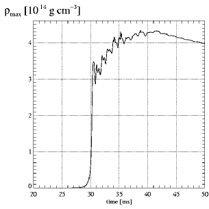
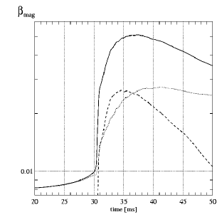
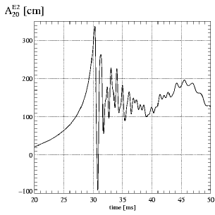
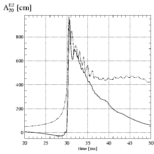
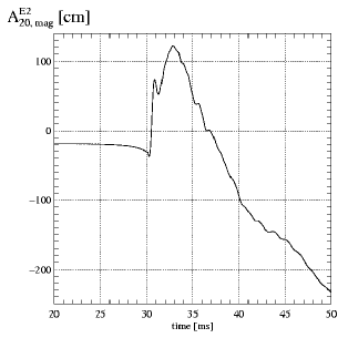
Figure 14: The dynamical evolution and the GW signal of model A3B3G5-D3M13. The upper panels display the temporal evolution of the rotational energy parameter $\beta_{\mathrm{rot}}$ (left), the maximum density $\rho_{\mathrm{max}}$ (middle), and the magnetic energy parameters (right; $\beta_{\mathrm{mag}}$ (solid line), $\beta_{\phi}$ (dashed line), and $\beta_{\mathrm{mag}}-\beta{\phi}$ (dotted line)), respectively. The GW signal of the model is shown in the lower panels: total amplitude (solid line, left), $-A^{\mathrm{E}2}_{20;\mathrm{hyd}}$ (solid line, middle), $A^{\mathrm{E}2}_{20;\mathrm{grav}}$ (dashed line, middle), and $A^{\mathrm{E}2}_{20;\mathrm{mag}}$ (right).

4.2.2 Models bouncing due to centrifugal forces

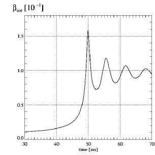
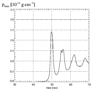
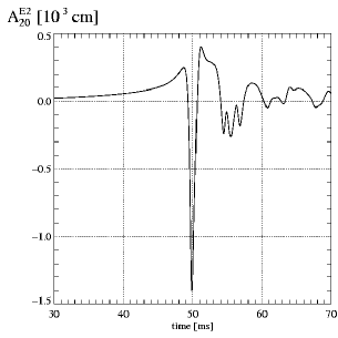
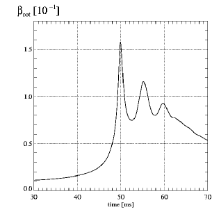
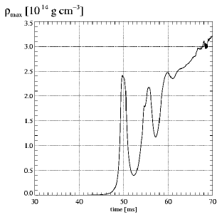
Figure 15: The evolution of the rotational energy parameter $\beta_{rot}$ (left panels), of the maximum density (middle panels) and the GW signal (right panels) of models A3B3G3-D3M10 (top panels), and A3B3G3-D3M12 (bottom panels), respectively.

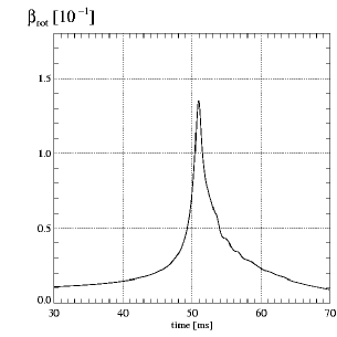
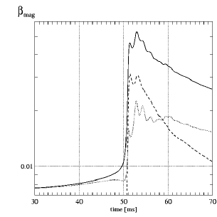
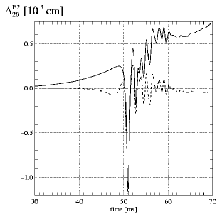
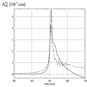
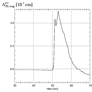
Figure 16: The dynamical evolution and the GW signal of model A3B3G3-D3M13. The upper panels display the temporal evolution of the rotational energy parameter $\beta_{\mathrm{rot}}$ (left), the maximum density $\rho_{\mathrm{max}}$ (middle), and the magnetic energy parameters (right; $\beta_{\mathrm{mag}}$ (solid line), $\beta_{\phi}$ (dashed line), and $\beta_{\mathrm{mag}}-\beta{\phi}$ (dotted line)), respectively. The GW signal of the model is shown in the lower panels: total amplitude (solid line, left; the dashed line gives the contribution of the layers with $r\leq 55.6\,$km), $-A^{\mathrm{E}2}_{20;\mathrm{hyd}}$ (solid line, middle), $A^{\mathrm{E}2}_{20;\mathrm{grav}}$ (dashed line, middle), and $A^{\mathrm{E}2}_{20;\mathrm{mag}}$ (right).

The weak–field models of series A3B3G3-D3Mm belong to the transition class between standard–type and centrifugally bouncing cores. They bounce mostly due to centrifugal forces and exhibit large–scale pulsations after bounce, but their maximum density exceeds nuclear matter density during bounce. Both the period and the damping of the pulsations are significantly larger than for purely centrifugally bouncing type-II models (Fig. 15). Their GW signal consists of a pronounced peak of negative amplitude at bounce, and subsequent relatively long–period oscillations.

For the strong–field variants of this model series, e.g. model A3B3G3-D3M12 (Fig. 15), the main evolutionary effect of the magnetic field is the extraction of rotational energy after bounce that proceeds on time scales much longer than the dynamic time scale of the inner core. Model A3B3G3-D3M12 reaches a maximum rotation parameter $\beta_{rot}^{\mathrm{max}}=0.16$ at bounce, which is nearly the same value as in the non–magnetic case. At the time of the second density maximum $\beta_{rot}$ is only slightly smaller than in the weak–field model A3B3G3-D3M10, but at the next (3rd) maximum the rotational energy has decreased by about $15\,\%$. Unlike in the weak–field model no fourth density maximum occurs. Instead, $\beta_{rot}$ decreases monotonically. The rotation rate of model A3B3G3-D3M12 is sufficiently large for a sufficiently long time to allow the core to exhibit several centrifugal pulsations before it settles down in a pressure supported final equilibrium state. During these pulsations the time–averaged value of $\rho_{\mathrm{max}}$ increases, and densities significantly larger than the bounce density $\rho_{b}=2.41\cdot 10^{14}\ \mathrm{cm\,s}^{-1}$ are reached.

The GW signal of the strong–field model A3B3G3-D3M12 is similar to that of the weak–field model A3B3G3-D3M10 during the first $\approx 10\ \mathrm{ms}$ after bounce when the cores of both models still undergo large–scale pulsations. Later when the rotational energy has decreased sufficiently and the pulsations begin to fade away, the signals begin to differ slightly. The maximum density now increases monotonically. Rotation is no longer important for the core’s stabilization, as it is supported by pressure forces. Thus, like in the case of a standard–type core (e.g. A1B3G3-DdMm), the rapid oscillations of the GW amplitude for $t\ga 60\mathrm{\ ms}$ occur on the core’s dynamic time scale. Superimposed to the oscillations is a positive mean amplitude $A^{\mathrm{E}2}_{20}\approx 100\mathrm{cm}$, which results from the enhanced asphericity of the shock wave as compared to that of the weak–field model.

The most strongly magnetized model of series A3B3G3-D3Mm, namely model A3B3G3-D3M13, behaves very differently from its weak–field variants as e.g. model A3B3G3-D3M10 (Fig. 15). Unlike the latter model it suffers a single bounce at $\rho_{b}=2.69\cdot 10^{14}\ \mathrm{cm\,s}^{-1}$ (a value about $10\,\%$ larger than for the weak–field models) with a subsequent contraction phase caused by the decrease of the core’s rotational energy. After bounce the maximum density reaches a value of $\rho_{\mathrm{max}}=3.3\cdot 10^{14}\ \mathrm{cm\,s}^{-1}$. Unlike model A3B3G3-D3M12, it does not exhibit any large–scale pulsations. Instead, it rapidly approaches a high density state without an intermediate phase where the density in the entire core is less that nuclear matter density, as it is the case for model A3B3G3-D3M12. The rotational energy ($\beta_{\mathrm{max}}=0.135$) is less than for models with weaker initial fields (e.g. $\,\beta_{\mathrm{max}}=0.16$ for model A3B3G3-D3M10), and decreases by $90\,\%$ within $15\,$ms (Fig. 16).

The collapse and post–bounce dynamics of model A3B3G3-D3M13 is similar to that of strong–field single–bounce models, as e.g. model A1B3G3-D3M13. Many features of the latter model are also present in model A3B3G3-D3M13: the bulb–like shock surface, the two highly magnetized post–shock regions (one near the equator and the other one along the polar axis), and a region of retrograde rotation near the equatorial plane at the edge of the inner core. The ratio of magnetic and gas pressure is largest at the axis at $r=175\ \mathrm{km}$ well behind the shock located at $r_{\mathrm{shock}}\approx 200\ \mathrm{km}$.

The GW signal of model A3B3G3-D3M13 is qualitatively similar to that of its less strongly magnetized variant A3B3G3-D3M12, but the features caused by the magnetic field are more pronounced (Fig. 16). The peak amplitude at bounce $A^{\mathrm{E}2}_{20}=-1128\ \mathrm{cm}$ is, contrary to model A3B3G3-D3M12, considerably less negative than in the weak-field model A3B3G3-D3M10 ($A^{\mathrm{E}2}_{20}=-1401\ \mathrm{cm}$). Immediately after bounce the GW signal shows certain similarities with that of model A1B3G3-D3M13 (Fig. 8): a large positive peak is followed by a series of oscillations occurring on the local dynamic time scale superimposed on an increase of the mean amplitude to a value of $A^{\mathrm{E}2}_{20}\approx 600\ \mathrm{cm}$ within $t\approx 5\ \mathrm{ms}$, which is the time it takes to turn the initially roughly spherical shock into a relatively wide bipolar outflow directed along the rotation axis.

Similar to cores bouncing due to pressure forces, the extraction of rotational energy from cores bouncing due to centrifugal forces proceeds qualitatively differently for models with an initial magnetic field strengths of $10^{12}\ \mathrm{G}$ and $10^{13}\ \mathrm{G}$, respectively. For the weaker field the extraction process relies on an instability–driven angular momentum transport, which is not required for the stronger field models.

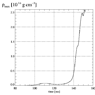
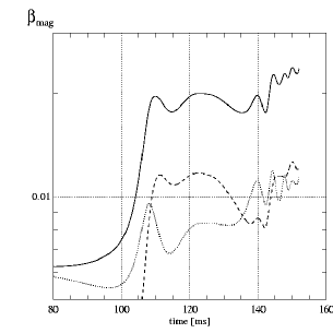
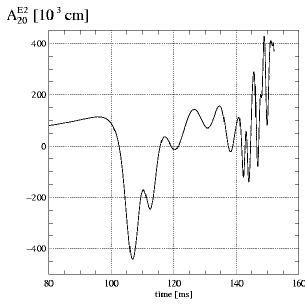
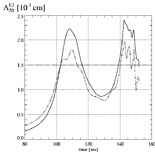
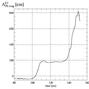
Figure 17: The dynamical evolution and the GW signal of model A2B4G1-D3M13. The upper panels display the temporal evolution of the rotational energy parameter $\beta_{\mathrm{rot}}$ (left), the maximum density $\rho_{\mathrm{max}}$ (middle), and the magnetic energy parameters (right; $\beta_{\mathrm{mag}}$ (solid line), $\beta_{\phi}$ (dashed line), and $\beta_{\mathrm{mag}}-\beta{\phi}$ (dotted line)), respectively. The GW signal of the model is shown in the lower panels: total amplitude (solid line, left), $-A^{\mathrm{E}2}_{20;\mathrm{hyd}}$ (solid line, middle), $A^{\mathrm{E}2}_{20;\mathrm{grav}}$ (dashed line, middle), and $A^{\mathrm{E}2}_{20;\mathrm{mag}}$ (right).

Unlike the other models, which collapse to higher densities when angular momentum transport by the magnetic field becomes dynamically important, model A2B4G1-D3M13 bounces at a lower density ($\rho_{\mathrm{b}}=6.84\cdot 10^{12}\ \mathrm{cm\,s}^{-1}$ compared to $\rho_{\mathrm{b}}=1.14\cdot 10^{13}\ \mathrm{cm\,s}^{-1}$ in the weak–field case). At bounce its rotational energy ($\beta_{\mathrm{max}}=0.093$) is less than that of model A2B4G1-D3M11 ($\beta_{\mathrm{max}}=0.118$), which has an initially 100 times weaker magnetic field. After bounce the rotational energy continues to decrease, and the core eventually suffers a second collapse that is stopped at $\rho_{\mathrm{max}}=2.5\cdot 10^{14}\ \mathrm{cm\,s}^{-1}$ (Fig. 17). During the second collapse $\beta_{\mathrm{rot}}$ rises temporarily slightly again, but angular momentum redistribution prevents the shock formed by centrifugal forces (at a similar density as the one resulting from the first bounce) from stopping the infall. Thus, a large fraction of the inner core continues to fall towards the center, until the collapse is halted by the stiffening of the equation of state, i.e. by a bounce due to pressure forces. A shock forms at the edge of the still very extended inner core ($r_{\mathrm{shock}}=70\ \mathrm{km}$ compared to $r_{\mathrm{shock}}\approx 10\ \mathrm{km}$ in the previously discussed models) at $t=108\ \mathrm{ms}$ at the beginning of the “plateau” in the evolution of $\rho_{\mathrm{max}}$ (see upper middle panel of Fig. 17), and it becomes slightly prolate. About 15 ms later ($t=123\ \mathrm{ms}$) this shock has reached a radius of $r_{\mathrm{shock}}\approx 200\ \mathrm{km}$ (Fig. 18). The magnetic field of model A2B4G1-D3M13 is less amplified and deformed than in the deeper collapsing single–bounce models such as e.g.  model A1B3G3-D3M13. The largest magnetic to gas pressure ratios are reached well behind the shock at about $0.75\,r_{\mathrm{shock}}\approx 400\ \mathrm{km}$.

The GW signal does not resemble any of the types used to classify non–magnetic models. Hence, we suggest to introduce a new type-IV GW signal (Fig. 17) which it is weaker at bounce ($A^{\mathrm{E}2}_{20}=-440\ \mathrm{cm}$) than in the non–magnetic case ($A^{\mathrm{E}2}_{20}=-610\ \mathrm{cm}$), but the amplitude remains large for a longer time period due to the longer phase of maximum contraction. Until the second collapse the signal varies on time scales ($\Delta t\approx 5\ \mathrm{ms}$) that are short compared to the pulsation periods of the non–magnetic case, but comparable to the sound crossing time of the relatively extended inner core. After $t\approx 140\ \mathrm{ms}$ the oscillation frequency and the amplitude of the GW signal strongly increases as the second collapse begins. During the entire post–bounce evolution the large negative gravitational and hydrodynamic (dominated by the centrifugal amplitude) contributions to the GW signal, and the large positive magnetic contribution add up to a total GW amplitude which is very small compared to the individual contributions.

Model A4B5G5-D3M13 bounces at a slightly higher maximum density ($\rho_{\mathrm{b}}=2.1\cdot 10^{14}\ \mathrm{cm\,s}^{-1}$) than its weak–field variant A4B5G5-D3M10 ($\rho_{\mathrm{b}}=1.97\cdot 10^{14}\ \mathrm{cm\,s}^{-1}$; Fig. 19). The maximum rotational energy at bounce is barely affected by the presence of the strong magnetic field, but it changes the density structure of the core completely in the subsequent evolution. Models A4B5G5-D3Mm ($m\leq 12$) maintain a toroidal density structure ($r_{\mathrm{tor}}\approx 40\ \mathrm{km}$) during their entire evolution (Sect. 4.1), but in model A4B5G5-D3M13 the density structure is changed by magnetic forces. Up to a few milliseconds after bounce ($t\la 32\ \mathrm{ms}$), the core of model A4B5G5-D3M13 evolves only marginally differently than its weak–field variants. Later, however, magnetic stresses transfer angular momentum from the still toroidal density distribution into the surrounding gas, whereby the torus transforms into a flattened configuration, which has its density maximum only slightly off–center (Fig. 20). During this phase, the core develops a retrograde rotating region near the equatorial plane. The core’s transformation process is associated with a large increase of its maximum density comparable with that occurring during the first collapse (Fig. 19).

During the second collapse, both the magnetic and the rotational energy of the core increase. The magnetic energy ($\beta_{\mathrm{mag}}=0.11$) exceeds that of the primary collapse ($\beta_{\mathrm{mag}}=0.078$), and the rotational energy exceeds slightly the limit for the dynamic instability of MacLaurin ellipsoids ($\beta_{\mathrm{rot}}\approx 0.275$), but only for about 1 ms. We note that the rotational energy reaches its maximum value well before the density does, which is different from all other models. Later on, the rotation parameter rapidly decreases well below the corresponding value of the non–magnetic case.

The shock has a very prolate shape at core bounce, its axis ratio being $\ga 2:1$. At large latitudes, the ratio of magnetic and gas pressure is largest well behind the shock ($r<0.75\ r_{\mathrm{shock}}\approx 110\ \mathrm{km}$; Fig. 21). Due to the rather extreme rotation of the model, the high latitudes of the core are strongly rarefied, and the shock propagates into a very thin medium near the axis, its structure remaining unchanged.

The GW amplitude of the weakly magnetized ($\approx$ non–magnetic) models A4B5G5-D3Mm ($m\leq 12$) is characterized by a very large negative amplitude at bounce ($A^{\mathrm{E}2}_{20}\approx-4100\ \mathrm{cm}$; Fig. 19 and Table 4). The signal is positive for several milliseconds after bounce due to the aspherical shock wave, and approaches zero rapidly after the violent re–expansion of the core. The bounce amplitude is significantly lowered ($A^{\mathrm{E}2}_{20}\approx-3470\ \mathrm{cm}$) in the strongly magnetized model A4B5G5-D3M13 (Fig. 19 and Table 4), immediately after bounce the GW amplitude is strongly positive and eventually becomes even more positive due to the growing asphericity of the shock wave. The secondary collapse of this models shows up in the GW amplitude in the form of a local minimum. Afterwards the amplitude rises to values $A^{\mathrm{E}2}_{20}>2000\ \mathrm{cm}$ and shows superimposed very weak oscillations with a period of slightly less than 1 ms. In this model, the magnetic and the combined hydrodynamic plus gravitational amplitude contributions show a clear phase shift resulting from the opposing actions of hydrodynamic (mainly centrifugal) and magnetic forces.

In all our models bouncing due to centrifugal forces the peak value of the GW signal at bounce decreases with increasing magnetic field strength, and for most models the ratio of the amplitudes of the post–bounce to the pre–bounce signal peaks decreases. Note that the latter statement must be considered carefully since – as discussed above – the GW signal may be subject to large modifications for models with very strong fields.

Figure 18: Model A2B4G1-D3M13 at $t=123.39\ \mathrm{ms}$ when the expansion of the core is maximum just prior to its second collapse. Besides the magnetic pressure (color shaded), the flow field (vectors), and the magnetic field lines are shown.

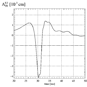
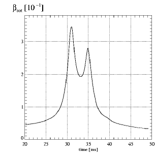
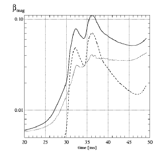
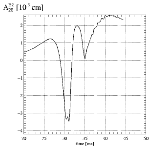
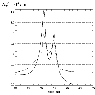
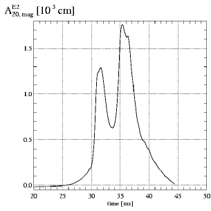
Figure 19: Evolution of the rotational energy parameter $\beta_{\mathrm{rot}}$ (left) and the maximum density (middle) of models A4B5G5-D3M10 (upper row) and A4B5G5-D3M13 (middle row), respectively. The total GW amplitude of model A4B5G5-D3M10 is shown in the upper right panel, and the evolution of the magnetic energy parameters, $\beta_{\mathrm{mag}}$ (solid), $\beta_{\phi}$ (dashed), and $\beta_{\mathrm{mag}}-\beta_{\phi}$ in the middle right panel, respectively. The panels in the bottom row show different contributions to the GW amplitude of model A4B5G5-D3M13: total amplitude ( left), $-A^{\mathrm{E}2}_{20;\mathrm{hyd}}$ (solid line, middle), $A^{\mathrm{E}2}_{20;\mathrm{grav}}$ (dashed line, middle), and $A^{\mathrm{E}2}_{20;\mathrm{mag}}$ (right).

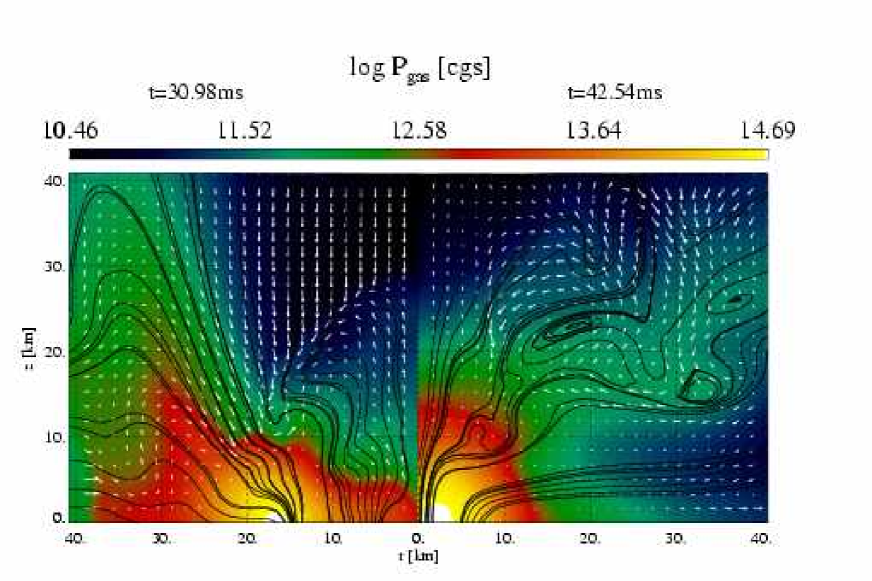
Figure 20: Comparison of two snapshots of model A4B5G5-D3M13. The innermost region of the core is displayed at $t=30.98\ \mathrm{ms}$ (at core bounce; left), and at $t=42.54\ \mathrm{ms}$ (right). The logarithm of the density (color–coded), the velocity (arrow), and the magnetic field lines are displayed, respectively.

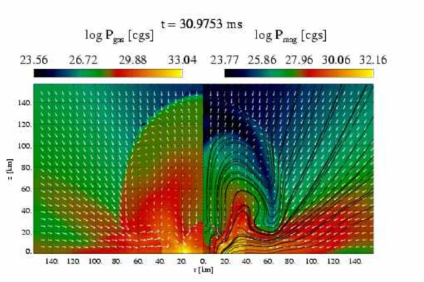
Figure 21: Model A4B5G5-D3M13 at $t=30.98\ \mathrm{ms}$ (core bounce). The flow field (vectors) and the magnetic field lines are displayed together with the gas pressure (color–coded, left) and the magnetic pressure (color–coded, right), respectively.

4.3 Magneto–rotational instability

The magneto–rotational instability (MRI) is a shear instability occurring in differentially rotating magnetized plasma, which generates turbulence that amplifies the magnetic field and transfers angular momentum (Balbus & Hawley, 1991, 1992, 1998). If effects due to buoyancy are neglected, a linear stability analysis shows that the condition for the instability of a mode with wavenumber $\@vec{k}$ is

$$\frac{\mathrm{d}\Omega^{2}}{\mathrm{d}\ln\varpi}+\left(\@vec{c}_{\mathrm{A}}\@vec{k}\right)^{2}<0\,,$$ (20)

where $\Omega$ is the angular velocity, $\varpi$ the distance from the rotation axis, and $\@vec{c}_{\mathrm{A}}\equiv{\@vec{b}}/{\sqrt{\rho}}$ the Alfvén velocity. When the magnetic field is very small (i.e. the Alfvén velocity is very small compared to both the local sound speed as well as the local rotation velocity) and/or the wavelength is very long, $\left(\@vec{c}_{\mathrm{A}}\@vec{k}\right)$ is negligible, i.e. the MRI occurs simply when the angular velocity gradient is negative (Balbus & Hawley, 1991, 1998):

$$\frac{\mathrm{d}\Omega^{2}}{\mathrm{d}\ln\varpi}<0\,.$$ (21)

The time scale of the fastest growing unstable mode is

$$\tau_{\mathrm{max}}=4\pi\left|\frac{\mathrm{d}\Omega}{\mathrm{d}\ln\varpi}\right|^{-1}\,,$$ (22)

which depends neither on the strength nor on the geometry of the magnetic field.

General theoretical considerations and non–linear simulations show that the magnetic energy achievable by the MRI field amplification process is of the order of the rotational energy, which is comparable to the saturation field expected from the process of winding–up field lines by differential rotation (Akiyama et al., 2003). However, in axisymmetric (non–linear) hydrodynamic simulations of accretion disks the field built up by the MRI was found to decay with a rate depending on the dissipation properties of the numerical scheme, and particularly on the grid resolution (Balbus & Hawley, 1991, 1998). This is due to Cowling’s anti–dynamo theorem (Shercliff, 1965) according to which an axisymmetric dynamo cannot work in a dissipative system, i.e. three–dimensional simulations are required.

In a star a convectively stable stratification will tend to stabilize the MRI, while convective instability will strengthen the MRI. Including the effects of buoyancy a mode with wave vector $\@vec{k}$ is unstable with respect to the MRI in a weakly magnetized rotating system, if the instability criterion

$$\left(\@vec{c}_{\mathrm{A}}\@vec{k}\right)^{2}<\left(\@vec{c}_{\mathrm{A}}\@vec{k}\right)^{2}_{\mathrm{crit}}\equiv-N^{2}-\frac{\mathrm{d}\Omega^{2}}{\mathrm{d}\ln\varpi}$$ (23)

is fulfilled (Balbus & Hawley, 1991; Balbus, 1995), where $N$ is the Brunt–Väisälä or buoyancy frequency. The wave number of the fastest growing mode is given by

$$\left(\@vec{c}_{\mathrm{A}}\@vec{k}\right)_{\mathrm{max}}^{2}=\Omega^{2}\left[1-\frac{(-N^{2}-\kappa^{2})^{2}}{16\Omega^{4}}\right]\,,$$ (24)

where $\kappa^{2}=4\Omega^{2}+\mathrm{d}\Omega^{2}/\mathrm{d}\ln\varpi$ is the epicyclic frequency. This mode grows exponentially with the time scale

$$\tau_{\mathrm{max}}=4\pi\left|\frac{N^{2}}{2\Omega}+\frac{\mathrm{d}\Omega}{\mathrm{d}\ln\varpi}\right|^{-1}\,,$$ (25)

which is a generalization of Eq. 22.

For decreasing wavenumber $k$ (provided that $kc_{\mathrm{A}}<(kc_{\mathrm{A}})_{\mathrm{max}}$) the maximum growth rate ($=2\pi/\tau_{\mathrm{max}}$) decreases approaching the value

$$\omega_{\mathrm{long}}^{2}=-N^{2}-\kappa^{2}$$ (26)

in the limit of very long wavelengths ($k\to 0$) independently of the Alfvén velocity. If the MRI occurs in a buoyantly stable stratification (where $N^{2}>0$), long modes will grow very slowly compared to the maximum growth rate. In the opposite case modes with a very small wave number grow very fast, and the growth rate of long modes will be of the order of the maximum growth rate. In the following discussion we use the names “magneto–shear” and “magneto–convective” limit to discriminate the two limiting cases without implying any deeper physical significance, because it is a matter of ongoing debate whether there exists a fundamental physical distinction between the two cases in the context of angular momentum transport in accretion disks (see, e.g. (Balbus & Hawley, 2002; Narayan et al., 2002)).

For a rotating magnetized configuration with axial symmetry the growth time scale of the maximum growing MRI mode in the presence of entropy gradients is given in spherical coordinates $(r,\theta)$ by Akiyama et al. (2003)

$$\tau_{\mathrm{MRI,en}}= 2 \pi\,\left|(\eta^{2}-2\eta+1)\Omega^{2}+\frac{\eta-1}{2}\left(\xi N^{2}+\eta\frac{\mathrm{d}\Omega^{2}}{\mathrm{d}\ln r}\right)\right.$$ (27)

$$+ \left.\frac{1}{16\Omega^{2}}\left(\xi N^{2}+\eta\frac{\mathrm{d}\Omega^{2}}{\mathrm{d}\ln r}\right)^{2}\right|^{-1/2}\,,$$

where

$$\eta^{2} = \left(1-\sin 2\theta\right)^{2}\,,$$ (28)

$$\xi^{2} = \sin^{2}\theta\,\left(1-\sin 2\theta\right)\,.$$ (29)

The additional subscript “en” refers to the entropy gradient included into Eq. 27 via the Brunt–Väisälä frequency. In the equatorial plane, where the polar angle $\theta=\pi/2$, the time scale given by Eq. 27 is equivalent to that obtained from Eq. 25.

In order to see the MRI in our simulations, we must have sufficient spatial resolution to resolve at least the modes with the longest wavelengths which grow fastest. However, as these modes have the smallest wavenumbers, the Alfvén velocity and thus the magnetic field (parallel to the direction of $\@vec{k}$) must be sufficiently large for the product $\@vec{c}_{\mathrm{A}}\cdot\@vec{k}$ to be in the range of maximum growth. This is unproblematic in the magneto–convective case due to the large growth rate in the limit $\@vec{c}_{\mathrm{A}}\@vec{k}\to 0$. In the magneto–shear limit only modes near $\left(c_{\mathrm{A}}k\right)_{\mathrm{max}}$ grow fast, which are, however, difficult to resolve. Further numerical complications arise from the fact that we have to identify the MRI in a very inhomogeneous and highly dynamical background flow.

Apart from the direct solution of the MHD equations, there are alternative ways to investigate the MRI and the turbulence driven by the instability, such as the inclusion of well-suited models for turbulent transport coefficients into the momentum and energy equations. Various closure models for magnetorotational turbulence exist. The ones by Ogilvie (2001, 2003) and Williams (2005, 2004) which make use of the analogy of MHD turbulence with viscoelastic flows as observed, e. g. in polymer fluids in the laboratory, seem particularly interesting. Such methods provide a way for including turbulence effects into a numerical simulation that cannot treat these effects due to, e. g. resolution or symmetry constraints. However, in the simulations we report here, we did not consider any of these models. Instead, we focussed on the possibility of directly simulating the development of the instabilities.

In most of our models we find extended MRI unstable regions at various epochs. During collapse the cores are unstable in the magneto–shear limit. However, the growth times are significantly larger than the collapse time scale: even for the fastest growing mode they are of the order of a second (in the initial models). As the rotational energy and the degree of differential rotation increase during collapse, the growth times become smaller, but remains larger than the time until bounce, i.e. the dynamical background evolves faster than any unstable mode. Hence, we do not observe the growth of the MRI even for models where the initial magnetic field is sufficiently strong for magneto–shear modes to be numerically resolved.

During and shortly after bounce the cores possess a convectively stable stratification, i.e. the MRI is of magneto–shear character. In model A1B3G3-D3M10 the immediate post–shock region is unstable shortly after shock formation due to a large negative angular velocity gradient (in $\varpi$–direction). The growth times are in the sub–millisecond to millisecond range, i.e. comparable to the dynamic time scales. The fastest growing modes correspond to spatial scales of less than $100\,$m, which are significantly smaller than the (local) grid resolution of $\sim 300\,$m. For models with a stronger magnetic field (e.g. A1B3G3-D3M12) the spatial scales of the fastest growing modes are larger due to the larger Alfvén velocity, and they can be resolved. However, they cannot be discriminated from the dynamic background flow at the time of bounce which is dominated by numerous pressure waves propagating through the inner core and launching the shock wave. Moreover, obscuring the action of the MRI, the strong shear flow surrounding the ”surface” of the inner core produces a strong toroidal magnetic field component. The positive entropy gradient behind the shock wave does not allow the MRI to grow in most of the post–shock region, while large parts of the inner core are MRI unstable throughout the entire post–bounce evolution due to the very flat entropy profile of the core. However, as the instability is of magneto–shear nature, one encounters the previously discussed spatial resolution problem unless the magnetic field is already quite strong. The maximum growth rates are moderate ($t_{\mathrm{grow}}\la 10\,$ms).

Well after bounce when the shock wave begins to weaken and thus (locally) negative entropy gradients develop, the MRI growth rates become large even for long wavelengths (magneto–convective limit). Thus, we observe the emergence of the corresponding modes, and a growth of the vorticity $\@vec{\omega}=\@vec{\nabla}\times\@vec{v}$ of the flow. However, this occurs late after bounce, when our assumptions concerning the microphysics do no longer hold. For model A1B3G3-D3M10, we can study the onset of magneto–convective modes. In regions where the growth times of the MRI modes (in the limit $k\to 0$) are less than $10\,$ms (Fig. 22), we find a rapid increase of the magnetic energy, the magnetic energy density, and of the specific magnetic energy. Their temporal variation can be described by exponential laws in the interval $57\,\mathrm{ms}\leq t\leq 96\,\mathrm{ms}$. In phases when the field is amplified by differential rotation only, the toroidal field increases but the poloidal field and the corresponding magnetic field energy stay approximately constant (Fig. 22). However, when the MRI sets in, the poloidal component grows too due to the stretching of the poloidal field lines by meridional motions. Because of this behavior the two field amplification mechanisms can be distinguished.

For initially very strong magnetic fields ($\ga 10^{12}\ \mathrm{G}$), the spatial scales of interest for the MRI can easily be resolved even in the magneto–shear limit, and the MRI criterion is fulfilled the growth rates being similar to those of the weak–field case. The proto–typical model A1B3G3-D3M12 shows the creation of a large amount of vorticity both in the post–shock gas and in the MRI unstable regions of the inner core (Fig. 7). Its vorticity is considerably larger than in the corresponding weak field model A1B3G3-D3M10, where we cannot resolve the growth of the unstable modes due to their very small spatial scales. The flow is organized in sheet–like structures which are typically a few kilometers wide in $\varpi$–direction and $\sim 10\,$km long in z–direction. Another prominent flow structure forms near the equatorial plane in the outer layers of the inner core, where a violent meridional flow leads to the largest amplification of the poloidal field and to angular momentum transport out of the inner core. The latter, which implies that the loss of the rotational support of the inner core is caused by the MRI, holds for all models where we can resolve the unstable modes, and where the field is not too strong initially. For the extreme models AaBbGg-D3M13 the stress tensor is initially already large enough for significant angular momentum transport to occur, i.e. only a very small amount of field amplification is required.

Initially weak magnetic fields should lead to a similar dynamical behavior, as the MRI does not depend on the initial field strength. The modes should grow on similar time scales, but smaller spatial scales. In practice, however, structures resolvable on our grid are much larger than the wavelengths of the fastest growing modes, i.e. they have relatively small growth rates. Hence, the development of the MRI is artificially delayed. In addition, the smaller scales of the more unstable modes may affect the global dynamics. Indeed, if we simulate the evolution of model A1B3G3-D3M11 for a longer time, the poloidal field energy starts to rise after $t\approx 65\,$ms. This rise is accompanied by the formation of a flow pattern consisting of sheets of large vorticity, and the extraction of rotational energy from the core, quite similar to our findings for model A1B3G3-D3M12, though less pronounced. Thus, the distinction between weak- and strong–field models may be irrelevant, because even small initial fields give rise to the same kind of instability and can become “strong” according to our criterion very rapidly.

The poloidal field strength oscillates similarly as the density or the rotational energy during the post–bounce phase for the models bouncing due to centrifugal forces. The field is subject to compression and expansion, but apart from the oscillations it does not grow unless an MRI–like mechanism sets in.

The magneto–convective motions found during the later stages of weak field models are much less pronounced in the cores of strong field ones. There are two reasons for this behavior: Firstly, due to the extraction of angular momentum from the core one of the driving forces of the instability is reduced, and secondly a strong magnetic field is known to suppress convection. The latter also holds for the MRI which is hampered by too strong fields, as the seed field cannot be amplified beyond the MRI saturation value. This can be seen from Eq. (23): For large Alfvén velocities only modes with very long wavelengths (or small wavenumbers) are unstable. If the critical wavelength exceeds the intrinsic scales of the problem, e.g. the size of the inner core or the size of potentially unstable regions, the unstable longer modes cannot develop, and the modes of smaller wavelengths are stable.

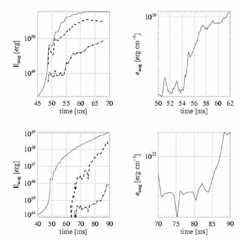
Figure 22: Comparison of the evolution of models A1B3G3-D3M12 (upper panels) and A1B3G3-D3M10 (lower panels). The left panels display the total magnetic energy (solid lines) of the core, and the total (dashed lines) and poloidal field energy (dash-dotted lines) of the MRI–unstable regions, which are defined according to two different criteria: For the strong–field model A1B3G3-D3M12 all zones are considered where the growth time of the fastest growing mode is less than $10\,$ms, while for the weak–field model A1B3G3-D3M10 the corresponding magneto–convective limit is used. The energy density $e_{\mathrm{mag}}=E_{\mathrm{mag}}/V$ of the poloidal field in the MRI–unstable regions is shown in the right panels. The poloidal field increases rapidly when the MRI grows, which happens in the strong–field model (top right) shortly after bounce, and in the weak–field model (bottom right) by magneto–convective modes at later epochs.

4.4 Influence of the magnetic-field configuration

The dynamics and gravitational wave signature of the models A3B3G5-DdM12 differing only in the location of the field–generating current loop (i.e. in their Dd parameter; see Sect. 2.3.3) are qualitatively quite similar, except for model A3B3G5-D0M12 whose current loop is located at infinity (see the discussion below). The time scale for the slow–down of the core exhibits some variation, but otherwise the evolution and the GW signal agree qualitatively quite well with those of the corresponding reference models A3B3G5-D3Mm (see above). This may be surprising because the initial total magnetic energies of models having uniform fields may be more than 100 times greater than that of current–loop models (table 2). However, the outer parts of the very extended field structure of the more strongly magnetized models, where most of the additional magnetic energy is stored, are dynamically less important than the central regions, and in particular the region around the field–generating current loop where the magnetic field is strongest.

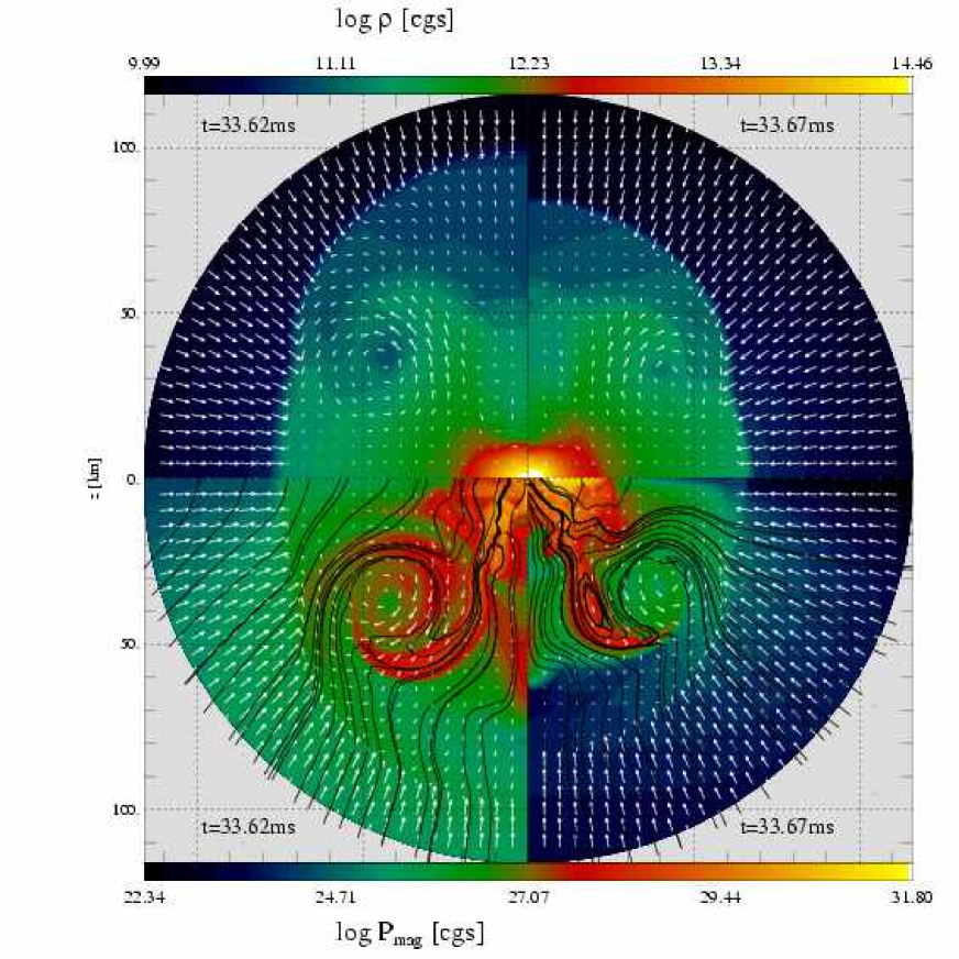
Figure 23: The post-shock region of models A3B3G5-D0M12 (left quadrants) and A3B3G5-D2M12 (right quadrants) at $t\approx 33.6\ \mathrm{ms}$ about 3 ms after core bounce. Density and magnetic pressure (color–coded) are displayed in the top and bottom quadrants, respectively. Additionally, the flow field (vectors) and the poloidal field lines of the magnetic field are displayed.

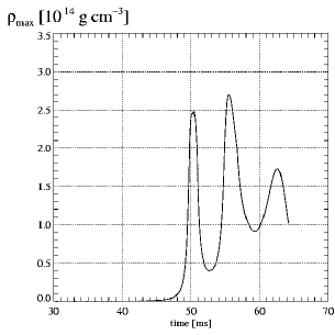
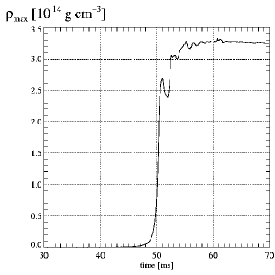
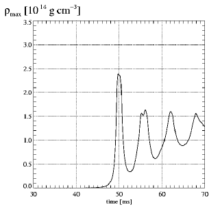
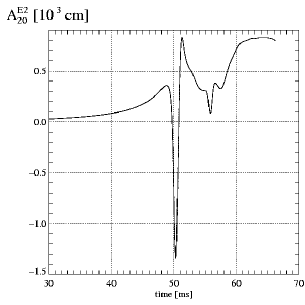
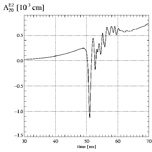
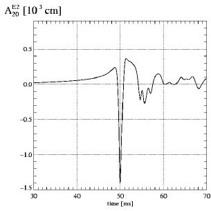
Figure 24: The evolution of the maximum density (top panels) and the GW amplitude (bottom panels) of models A3B3G3-D0M13 (left panels), A3B3G3-D3M13 (middle panels), and A3B3G3-D1M13 (right panels), respectively. The GW signal of model A3B3G3-D0M13 shows a constant offset from zero, which is subtracted here.

For the initially homogeneously magnetized model A3B3G5-D0M12 a less efficient braking of the core’s rotation is observed than for the corresponding current-loop models. Instead of a contracting secularly, the core expands to sub–nuclear densities on a comparable time scale. The rotation energy of the immediate post–bounce core of model A3B3G5-D0M12 is slightly smaller ($\beta_{\mathrm{rot}}\approx 0.076$ at $t\approx 32\ \mathrm{ms}$) than for the corresponding non–magnetic core ($\beta_{\mathrm{rot}}\approx 0.084$ at $t\approx 32\ \mathrm{ms}$), and it decreases sightly during the subsequent evolution. Although the magnetic field gets amplified a little during collapse, $\beta_{\mathrm{mag}}$ decreases until bounce because most efficient amplification takes place in the central regions of the core whereas the total magnetic energy is dominated by the outer regions where the field stays roughly constant during collapse. Afterwards, both $E_{\mathrm{mag}}$ and $\beta_{\mathrm{mag}}$ show a comparable growth to the current–loop models, and the ratio of toroidal field energy and total field energy grows steadily, but slowly. The magnetic field of the uniformly magnetized core has a simpler structure at late times, while the current–loop fields become more and more twisted. The gravitational wave amplitude of model A3B3G5-D0M12 is strongly dominated by the fluid contribution in spite of its large initial magnetic energy, and resembles that of the corresponding current-loop cores in many respects. The small magnetic contribution to the signal never exceeds that of model A3B3G5-D3M12, although this model has a 15 times smaller magnetic energy (but the same central field strength).

Model A3B3G5-D2M12 has an initial magnetic field energy which is a factor of 150 greater than that of model A3B3G5-D0M12 (table 2). Nevertheless, at $t\approx 39\ \mathrm{ms}$, its magnetic field is almost three times as energetic as that of model A3B3G5-D0M12 ($\beta_{\mathrm{mag}}=0.0075$ compared to $\beta_{\mathrm{mag}}=0.0028$) due to the different amount of field amplification occurring in both cases. At bounce both models have developed a region of high magnetization near the edge of the inner core close to the rotation axis. In model A3B3G5-D2M12 this region also extends towards larger radii along the equatorial plane forming a highly magnetized “sheet” which is a relic of the initially highly magnetized region around the field generating current–loop. The shape of the shock waves is similar in both models, but the regions of large magnetic pressure are more extended in the current–loop model filling the whole post–shock region, whereas they are more concentrated towards the very center of the core for the uniform field model (Fig. 23).

Similar trends as for model series A3B3G5-DdM12 can be observed in the case of model series A3B3G3-DdM13 (Fig. 24). The dynamics of the current–loop model A3B3G3-D1M13 is qualitatively comparable to that of a A3B3G3-D3Mm model with a much weaker magnetic field. Hence, its GW signal does not differ much from the non–magnetic case in spite of its strong initial magnetic field. However, we find large differences between the uniform field model A3B3G3-D0M13 (Fig. 24, left panels) and the current–loop models, as e.g. A3B3G3-D3M13 (Fig. 24, middle panels). The maximum density of the former model exhibits large–scale pulsations during which the bounce density is exceeded by $9\,\%$, and $\rho_{\mathrm{max}}$ is smaller than $\rho_{\mathrm{nuc}}$ for most of the time. The core has a very high magnetic energy initially, $\beta_{\mathrm{mag}}\approx 20\,\%$, which decreases during the collapse until it levels off at $\approx 7\,\%$. This value is still much larger than the largest one reached by the current–loop models during their whole evolution. The GW signature of model A3B3G3-D0M13 reflects the density oscillations of the core, and like in the case of model A3B3G3-D3M13, it is considerably shifted towards positive amplitudes (Fig. 24) due to the very aspherical shape of the shock wave.

5 Summary and conclusions

Past and present realistic studies of core collapse supernovae neglect magnetic fields. Instead, they focus on an elaborate and accurate description of the microphysics and (neutrino) transport physics. Since this is a formidable task requiring extensive computational resources, these studies are necessarily limited to a very small number of different initial models. Bearing in mind our lack of knowledge of the exact conditions in the pre–collapse star, we pursued a complimentary approach. Instead of simulating the evolution of a few stars in great detail, we performed a comprehensive parameter study covering the space of possible progenitors with a large number of initial models and exploring a relatively unknown territory, namely the influence of magnetic fields. Consequently, we are restricted to some simplified and approximate treatment of the core’s physics, and employ only simplified progenitor models (i.e. polytropes).

Our parameter study focuses on the investigation of two main questions:

• How do magnetic fields affect the dynamics of the collapse and bounce, and how is their presence reflected in the gravitational wave signal emitted by the core?

• Which pre–collapse magnetic fields (strength and geometry) and angular momentum (amount and distribution) will cause important dynamic effects for core collapse?

To address these questions we have performed the most comprehensive parameter study of magneto–rotational core collapse up to now. We simulated the gravitational collapse and the immediate post–bounce evolution of a series of differentially rotating, magnetized, axisymmetric stellar core models using a newly developed 2D Newtonian MHD code based on the algorithm of Pen et al. (2003) that employs the relaxing TVD scheme of Jin & Xin (1995) and the constraint–transport method (Evans & Hawley, 1988) to keep the magnetic field divergence–free. Our code, which has been comprehensively tested, incorporates an analytic equation of state describing in an approximate way the thermodynamic properties of core matter (Janka et al., 1993). We also computed the gravitational wave signal produced by the core with the Einstein quadrupole formula taking into account both the contributions of the hydrodynamic and gravitational forces (Mönchmeyer et al., 1991), and of the Lorentz forces (Kotake et al., 2004b). The initial models used in our study are identical to those used by Zwerger & Müller (1997) and Dimmelmeier et al. (2002a, b). The initial magnetic field is purely poloidal.

Our simulations show significant modifications of the dynamics and the GW signal of strongly magnetized cores compared to non–magnetic ones. Magnetic fields are amplified in some of our models to very large field strengths which are in the magnetar range ($|\@vec{B}|\sim 10^{15}\ \mathrm{G}$). Such strong magnetic fields efficiently extract rotational energy from the central core, thereby triggering a secular post–bounce contraction phase. They also cause the formation of collimated outflows, which give rise to distinctive features in the GW signal. Hence, it is in principle possible to extract information about the degree to which an explosion has a jet–like character from the GW signal. Further specific results are:

1. From the initially purely poloidal magnetic field, large toroidal field components are created by the action of the differentially rotating core in a so–called $\Omega$ dynamo, the energy of the saturation field being of the order of the rotational energy of the core. The efficiency of this field winding process depends on the angular momentum distribution of the progenitor and the amount of differential rotation arising during collapse. The latter is determined by the degree of non–homologous collapse which is sensitively influenced by the equation of state and the rotation rate. The saturation fields estimated from the rotational energy of our collapsed cores are of the order of $10^{15}\ \mathrm{G}$, which are field strengths expected for magnetars, but not for typical neutron stars. The field amplification process is found to be less efficient if some magnetic energy is consumed for the acceleration of matter by dynamically important fields.

2. As MHD instabilities acting on the toroidal field component are suppressed due to the assumed axisymmetry, we are unable to simulate the corresponding field amplification processes, and thus may underestimate the saturation value and the growth rate of the magnetic field. However, if the entire dynamo process of transforming poloidal and toroidal fields into one another and their amplification is mainly driven by differential rotation, the saturation fields and the growth rates are expected not to exceed those found in our simulations. We point out that (i) without any symmetry restriction fields of similar strengths may arise when one evolves initially less magnetized cores, and (ii) that the strong initial fields of our progenitors (which are stronger than those expected in actual cores) may compensate for a possible additional dynamo action unconsidered in our models. The field amplification is fastest for rapidly and very differentially rotating models. In models producing a type-I GW signal the magnetic field is amplified more efficiently than both in the faster collapsing models of type-III and the centrifugally bouncing type-II models.

3. The influence of a magnetic field on the dynamics and the GW signature of the core depends mainly on the initial magnetic field strength, and to a lesser extent on the field topology. For the weakest of our initial fields ($B\sim 10^{10}\ \mathrm{G}$) we do not find any significant impact either on the dynamics or on the GW signal on the time scales covered by our simulations ($\la 100\ \mathrm{ms}$ after core bounce). However, sufficiently strong fields have a large impact on the dynamics of the core and on the gravitational wave signal. Compared to the corresponding non–magnetized models, the core bounce is somewhat delayed for the majority of our very strongly magnetized models ($B\ga 10^{12}\ \mathrm{G}$), and the bounce density is slightly enhanced. Extremely strong initial magnetic fields ($B\ga 10^{13}\ \mathrm{G}$) efficiently slow down the rotation rate of the central core already during collapse, and thus reduce its. centrifugal support by a considerable amount. Due to the loss of angular momentum from its central regions the core eventually begins to contract or even enters a second collapse phase after bounce. Hence, an initially extremely magnetized and rapidly rotating core, which bounces due to centrifugal forces at low densities, evolves into a very compact configuration that is almost entirely pressure supported, its initially toroidal density stratification changing into a flattened centrally concentrated one.

4. The magnetic stresses of the toroidal field component (created by the differential rotation) can cause a strong pinch effect, which gives rise to a mildly relativistic, jet–like outflow along the rotation axis, and consequently to a very prolate shock wave. The aspherical outflow is mainly driven by the very high magnetic pressure in the post–shock plasma, as first pointed out by Yamada & Sawai (2004), and it is observed both in cores that bounce due to the stiffening of the EOS and (mainly) due to centrifugal forces. In purely hydrodynamic calculations highly aspherical outflows are only encountered for very extreme rotators, whereas they are quite common for models with an initial magnetic field strength of $B\ga 10^{13}\mathrm{G}$. On somewhat longer time scales, similar but weaker outflows are observed for models having only a tenth of this field strength. This finding might be of relevance for the study of Gamma–Ray Bursts. According to our results extreme initial conditions are required for the formation of jet–like outflows on the time scale of a few ten milliseconds. However, our results may also apply on longer time scales to the smaller rotation rates and the weaker magnetic field strengths of more realistic stellar progenitors.

5. All simulated cores develop MRI unstable regions. However, in most cases, a fast growth of the MRI is limited to short–wavelength modes which we cannot resolve due to insufficient numerical resolution. For initial fields $\ga 10^{12}\ \mathrm{G}$, the fastest growing modes have sufficiently long wavelengths to be resolved numerically. A meridional flow pattern characterized by large vorticity arises the circulation pattern being organized in sheet–like structures which is also the topology of the poloidal field. In contrast to the weak–field case, where we cannot resolve possibly unstable modes and where the poloidal field stays roughly constant after bounce, the poloidal field energy of strongly magnetized cores grows approximately exponentially. The field strengths found in our simulations are of the order of the saturation field estimates derived for the MRI, i.e. $\sim 10^{15}\ \mathrm{G}$ at the surface of the inner core. The growth of the field comes along with the transport of angular momentum out of the inner core, and thus a loss of rotational support. Consequently, the maximum density of the core rises steadily during the post–bounce evolution.

6. The gravitational wave signature of the core is altered significantly in the presence of initially strong ($B\ga 10^{12}\ \mathrm{G}$) magnetic fields compared to the corresponding non–magnetic case. Since pressure–bouncing type-I and type-III models are affected only quantitatively by strong magnetic fields (in contrast to the centrifugally bouncing models where magnetic fields change the collapse dynamics considerably), the GW amplitude of a strongly magnetized type-I or type-III model does not deviate strongly from the purely hydrodynamic case. Depending on the actual rotational profile and the EOS, the GW bounce amplitude may be enhanced or weakened by a few $10\,\%$. This confirms the findings of Yamada & Sawai (2004) obtained for a much smaller set of models.

7. For most strongly magnetized models we observe a shift of the bounce signal towards more positive amplitudes. A major part of this shift is due to magnetic forces: around the time of core bounce the magnetic part of the GW amplitude is positive and large indicating that the magnetic stresses act to diminish the core’s oblateness. This reduces the absolute value of the pronounced (negative) bounce amplitude for most type-I and type-II models, and enhances the (positive) maximum GW amplitude of the type-III models reached shortly before or after bounce. In the latter models strong magnetic fields also decrease the size of the much less pronounced (negative) bounce minimum of the GW amplitude. Rigidly and modestly fast rotating type-I models behave differently, as for these models the size of the (negative) bounce peak is enhanced significantly for initially extremely strong magnetic fields ($\sim 10^{13}\mathrm{G}$). After bounce, both the gravitational and the hydrodynamic parts of the GW amplitude decrease as the rotational flattening of the central core diminishes due to the extraction of angular momentum. Later in the evolution the magnetic part of the GW amplitude, now becoming increasingly negative, dominates the hydrodynamic one for cores which are slowed down very strongly. As in the case of purely hydrodynamic models, the GW signal of a strongly magnetized core bouncing due to pressure forces exhibits oscillations with periods that are comparable to the local dynamic time scale.

8. The dynamics of type-II models bouncing due to centrifugal forces is changed completely by the presence of strong magnetic fields. This is reflected in a rather drastic change of the GW signal emitted by these cores. As the large–scale pulsations of the core fade away during the secular contraction phase, the long–period modes of the GW signal become less important. Instead high frequency oscillations, similar to the ones emitted by type-I models, dominate the GW signal. The corresponding periods are given by the local dynamic time scales of the core which is no longer supported by rotation, but – at much higher densities – by pressure forces. This shift in the frequency of the GW amplitude provides observational evidence of the change of the core’s dynamics and structure by a strong magnetic field. We introduce the new GW signal type IV to refer to this phenomenon.

9. Aspherical outflows and shock waves get imprinted on the GW signal the signature being a large, slowly varying positive GW amplitude. A few ($\sim 5$) milliseconds after bounce, we find amplitudes of the order of $A^{\mathrm{E}2}_{20}\sim 10^{2}\ \mathrm{cm}$ which remain at roughly this level until the end of our calculations. As bipolar outflows occur preferentially in strongly magnetized cores, the GW signal may be used to distinguish strongly magnetized cores from non–magnetic or weakly magnetized ones.

The applicability of our findings to the supernova problem is limited by our simplified treatment of the microphysics (approximate equation of state), by the neglect of neutrino transport, and by our simplified and probably too extremely rotating and magnetized initial models. Nevertheless, after having shown that our code is suited for multi-dimensional MHD simulations of core collapse, and after having highlighted some general trends of magneto–rotational core collapse, we are ready for a more sophisticated investigation of the phenomenon. In particular, the evolution of our (more realistic) weak–field models on longer time scales will be the topic of further studies, as on longer time scales even initially weak magnetic fields can be amplified, e.g. by means of the magneto–rotational instability, to a strength relevant both for the dynamics and the GW signature of the core. Furthermore, the interplay of magnetic fields and various hydrodynamic instabilities occurring in a supernova explosion is a challenging topic to be addressed. In particular, the convective region between the proto–neutron star and the stalled hydrodynamic shock wave might be an arena where generic MHD effects such as the magneto–rotational instability do operate.

Imposing axial (and equatorial) symmetry is a serious restriction when simulating MHD flows. It prevents us from investigating the fate of cores whose magnetic field and rotational axis are misaligned as in pulsars, and from simulating the intrinsically 3D magneto–rotational instability to the full extent. We think that the first shortcoming will influence our results only slightly, as the initial magnetic field is soon completely dominated in our models by the field generated by differential rotation. Thus, provided there is a poloidal seed field of similar strength no significant changes are to be expected. The second restriction is probably uncritical for the relatively short time scales covered by our simulations, as the dominant amplification process for the magnetic field during these early stages is the rapid winding–up of the initial poloidal field by means of differential rotation. Additional field growth by the MRI or other MHD instabilities is probably less important. In any case, limited by the present computational resources, a 3D MHD parameter study of core collapse is still some years ahead.

A further limitation arises from our Newtonian approach, as we observe outflow velocities in some of our models that exceed $\sim 30\,\%$ of the speed of light and that are still increasing when we had to stop our simulations. Although being only mildly relativistic in our models, a study of the further evolution of these outflows may require a special relativistic MHD code, if the jets continue to accelerate. The effects of general relativistic corrections of the gravitational potential on magneto–rotational core collapse arising due to the high compactness of the collapsed cores have been investigated by us in some detail. The results of this complementary study will be presented in a separate publication.

Appendix A Relaxing TVD

In this section we summarize the basics of the relaxing TVD method. For further information the reader is referred to Pen et al. (2003); Jin & Xin (1995); Trac & Pen (2003).

A major drawback of MUSCL–type and Riemann solver schemes for systems of non–linear conservation laws is the need for calculating the eigenvalues $a_{m}$, and the eigenvectors of the Jacobian of the flux vector (Hebrew indices $(\aleph=1,\ldots,m)$ enumerate the components of the system of $m$ equations)

$$J^{\aleph\beth}=\frac{\partial F^{\aleph}}{\partial U^{\beth}}\,,$$ (30)

which usually is a computationally quite demanding step. This difficulty can be overcome by employing a relaxing TVD scheme (Jin & Xin, 1995; Trac & Pen, 2003) that does not require the explicit calculation of the eigenvectors of the system, and in some cases of most of the eigenvalues. The numerical method we have applied turns out to be both robust and accurate, and is well suited for simulations of core collapse. This is good news, as the method involves several considerable simplifications compared to more elaborate methods based on Riemann solvers, which make it computationally very cheap, and hence attractive. One replaces the one–dimensional system of conservation laws

$$\partial_{t}U^{\aleph}+\nabla F^{\aleph}=0$$ (31)

with the initial condition $U^{\aleph}(\xi,0)=U^{\aleph}_{0}(\xi)$ by the relaxation system

$$\partial_{t}U^{\aleph}+\nabla V^{\aleph}=0\,,$$ (32)

$$\partial_{t}V^{\aleph}+A^{2}\nabla U^{\aleph}=-\frac{1}{\tau}(V^{\aleph}-F^{\aleph})\,,$$ (33)

with the initial conditions $U^{\aleph}(\xi,0)=U^{\aleph}_{0}(\xi)$ and $V^{\aleph}(\xi,0)=F^{\aleph}(U^{\beth}_{0}(\xi))$. The constant $\tau$ is called the relaxation rate. The constant matrix $A=\textrm{diag}(a_{1},...,a_{m})$ satisfies the sub-characteristic condition

$$A^{2}-J^{2}\geq 0\,.$$ (34)

Thereby, the non–linear system (31) gets replaced by a system of linear equations that can be solved without the need of Riemann solvers. In the zero relaxation limit $\tau\to\infty$, one arrives at the relaxed system

$$\partial_{t}U^{\aleph}+\nabla V^{\aleph}=0\,,$$ (35)

$$\partial_{t}V^{\aleph}+A^{2}\nabla U^{\aleph}=0\,,$$ (36)

where $V^{\aleph}=F^{\aleph}(U^{\beth})$. Introducing right (R) and left (L) moving variables,

$$U^{\aleph;R,L}=\frac{1}{2}\cdot(U^{\aleph}\pm A^{-1}F^{\aleph})$$ (37)

the system decouples yielding

$$\partial_{t}U^{\aleph;R,L}\pm\nabla(AU^{\aleph;R,L})=0\,.$$ (38)

These two systems (R, L) of equations have the structure of linear advection equations for rightward and leftward directed advection, respectively. The constant advection velocities in both systems of equations are given by

$$c_{\aleph}^{R,L}=\pm a_{\aleph}\,.$$ (39)

Being of a quite simple structure and having quite simple characteristics with constant speeds $c_{\aleph}^{R,L}$, the system (38) can easily be solved using a first- or second–order accurate upwind scheme. The upwind fluxes at the zone interface $\mathcal{S}_{i+1/2}$ will be computed from variables of zone $\mathcal{Z}_{i}$ for the right–moving variable $U^{\aleph;R}$, and from zone $\mathcal{Z}_{i+1}$ for $U^{\aleph;L}$, respectively. The value of $U^{\aleph}$ can then be recovered from $U^{\aleph;R,L}$ by

$$U^{\aleph}=\frac{1}{2}(U^{\aleph;R}+U^{\aleph;L})\,.$$ (40)

As Jin & Xin (1995) showed, the resulting scheme will be TVD, if the sub-characteristic condition (34), and the CFL condition arising form the advection terms are fulfilled.

Appendix B Convergence tests

To ensure the numerical convergence of our results, we performed a number of simulations of the same model using different grid spacings. Based on these simulations, we selected a grid of 380 zones in radial and 60 zones in angular direction as our standard grid. The grid is logarithmically spaced in radius, with a central resolution of $(\Delta_{r})_{\mathrm{c}}\approx 300\ \mathrm{m}$ and a relative increase of the cell size from zone to the zone of $\approx 1.1\,\%$. The angular grid is uniform.

Results from a sample of the convergence runs are displayed in Fig. 25. We show the temporal evolution of the maximum density, the GW amplitude, and $\beta_{\mathrm{rot}}$ for model A1B3G3-D3M13, computed with grids of

• 280 zones in radius and $(\Delta_{r})_{\mathrm{c}}\approx 600\ \mathrm{m}$, and 30 zones in angle (dotted lines),

• standard resolution as described above (solid lines), and

• 580 zones in radius and $(\Delta_{r})_{\mathrm{c}}\approx 150\ \mathrm{m}$, and 90 zones in angle (dashed lines).

We compare both local properties of the models such as the maximum density of the core, and global ones such as the GW signal and the evolution of $\beta_{\mathrm{rot}}$. The results of these simulations indicate that our standard resolution is adequate to follow the evolution of our models.

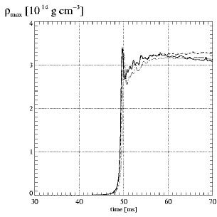
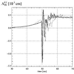
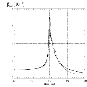
Figure 25: The temporal evolution of the maximum density, the GW signal and the rotational energy parameter $\beta_{\mathrm{rot}}$ of model A1B3G3-D3M13 comparing simulations with grids of different resolution. Results from a run with the standard grid of 380 logarithmically spaced zones in radius (central resolution of 300 m) and 60 zones uniformly distributed over $0\leq\theta\leq\pi/2$ are shown by the solid lines, and runs using a coarser grid of 280 zones in radius (central resolution of 600 m) and 30 zones in angle and a finer grid of 580 zones (central resolution of 150 m) and 90 zones in angle are plotted with dotted and dashed lines, respectively.

Appendix C Gravitational-wave extraction

Since we do not evolve the consistent set of general–relativistic MHD equations, we are not able to extract the GW signal from the metric. But, in the post–Newtonian limit, it is still possible to extract the lowest–order terms of the GW signal from the hydrodynamic variables. For this purpose we have used the reformulation of the quadrupole formula by Mönchmeyer et al. (1991), where temporal derivatives are replaced by spatial ones using the continuity and the Euler equations. Thus, the hydrodynamic fluxes and source terms are introduced into the quadrupole formula.

As we use spherical coordinates $(r,\theta,\phi)$ in our simulations, the metric perturbation associated with a gravitational wave is most conveniently expanded in terms of pure spin tensor harmonics $T^{\mathrm{E}2,lm}_{ab}$ and $T^{\mathrm{B}2,lm}_{ab}$ with the corresponding “electric” and “magnetic” amplitudes $A^{\mathrm{E}2}_{20}$ and $A^{\mathrm{B}2}_{20}$, respectively:

$$h_{ab}=\frac{1}{R}\sum_{l=2}^{\infty}\sum_{m=-l}^{+l} \left[A^{\mathrm{E}2}_{lm}\left(t-\frac{R}{c}\right)T^{\mathrm{E}2,lm}_{ab}(\theta,\phi)+\right.$$ (41)

$$\left.+A^{\mathrm{B}2}_{lm}\left(t-\frac{R}{c}\right)T^{\mathrm{B}2,lm}_{ab}(\theta,\phi)\right].$$

Under the assumption of axisymmetry, the only non–vanishing amplitude is $A^{\mathrm{E}2}_{20}$, which is given by (Mönchmeyer et al., 1991):

$$A^{E2}_{20}=\frac{\mathrm{d}^{2}}{\mathrm{d}t^{2}}M^{\mathrm{E}2}_{20}=\frac{\mathrm{d}}{\mathrm{d}t}N^{\mathrm{E}2}_{20},$$ (42)

where the radiative quadrupole moment $M^{\mathrm{E}2}_{20}$ is ($z=\cos\theta$) defined as

$$M^{\mathrm{E}2}_{20}=\frac{G}{c^{4}}\frac{32\pi^{3/2}}{\sqrt{15}}\int_{0}^{1}\mathrm{d}z\int_{0}^{\infty}\mathrm{d}\frac{r^{3}}{3}\rho(r,z,t)r^{2}\left(\frac{3}{2}z^{2}-\frac{1}{2}\right).$$ (43)

Using the continuity equation, the first time derivative of $M^{\mathrm{E}2}_{20}$ is given by

$$N^{\mathrm{E}2}_{20}=\frac{G}{c^{4}}\frac{32\pi^{3/2}}{\sqrt{15}}\int_{0}^{1}\mathrm{d}z\int_{0}^{\infty}\mathrm{d}\frac{r^{3}}{3}\rho r\left[v_{r}\left(\frac{3}{2}z^{2}-1\right)-3v_{\theta}z\sqrt{1-z^{2}}\right]\,.$$ (44)

The time derivative of $N^{\mathrm{E}2}_{20}$ is computed using the MHD momentum equation which allows ones to eliminate $\frac{\mathrm{d}}{\mathrm{d}t}(\rho v_{r},\rho v_{\theta})$ with the help of the hydro-magnetic and gravitational force terms given by

$$F^{r}_{\mathrm{MHD}} = -\frac{\partial r^{2}F_{rr}}{\partial r^{3}/3}-\frac{1}{r}\frac{\partial\sin\theta F_{r\theta}}{\partial(-\cos\theta)}+{}$$ (45)

$$+ \frac{1}{r}(2P_{\star}+\rho v_{\theta}^{2}-b_{\theta}^{2}+\rho v_{\phi}^{2}-b_{\phi}^{2}),$$

$$F^{\theta}_{\mathrm{MHD}} = -\frac{\partial r^{2}F_{\theta r}}{\partial(r^{3}/3)}-\frac{1}{r}\frac{\partial\sin\theta F_{\theta\theta}}{\partial(-\cos\theta)}+{}$$ (46)

$$+ \frac{\cot\theta}{r}(P_{\star}+\rho v_{\phi}^{2}-b_{\phi}^{2})-\frac{(\rho v_{r}v_{\theta}-b_{r}b_{\theta})}{r},$$

$$F^{r}_{\mathrm{grav}} = -\rho\partial_{r}\Phi,$$ (47)

$$F^{\theta}_{\mathrm{grav}} = -\frac{1}{r}\rho\partial_{\theta}\Phi\,.$$ (48)

The components of the flux tensor in the above expressions are given by

$$F_{ab}=\rho v_{a}v_{b}+P_{\star}\delta_{ab}-b_{a}b_{b}.$$ (49)

Following the derivation of the quadrupole formula by (Mönchmeyer et al., 1991), one then finds

$$A^{\mathrm{E}2}_{20} = \frac{G}{c^{4}}\frac{32\pi^{\frac{3}{2}}}{\sqrt{15}}\int_{0}^{1}\mathrm{d}z\int_{0}^{\infty}\mathrm{d}\frac{r^{3}}{3}$$ (50)

$$\left[f_{rr}(3z^{2}-1)+f_{\theta\theta}(2-3z^{2})-f_{\phi\phi}-6f_{r\theta}z\sqrt{1-z^{2}}-\right.$$

$$\left.-r\partial_{r}\Phi(3z^{2}-1)+3\partial_{\theta}\Phi z\sqrt{1-z^{2}}\right]\,,$$

where the components of $f_{ij}$ are given by

$$f_{ij}=\rho v_{i}v_{j}-b_{i}b_{j}\,.$$ (51)

The total isotropic pressure $P_{\star}$ (sum of the gas pressure and the magnetic pressure) cancels out, i.e. only the velocities and the magnetic stresses appear in the hydro-magnetic part of the amplitude.

Eq. 50 corresponds to the hydrodynamic and the Lorentz force parts of the quadrupole formula given by Kotake et al. (2004b), who derived the following expression for the GW amplitude $A^{\mathrm{E}2}_{20}=A^{\mathrm{E}2}_{20;\mathrm{hyd}}+A^{\mathrm{E}2}_{20;\mathrm{Lorentz}}+A^{\mathrm{E}2}_{20;\mathrm{mag}}$:

$$A^{\mathrm{E}2}_{20;\mathrm{hyd}}(t) = \frac{G}{c^{4}}\frac{16\pi^{\frac{3}{2}}}{\sqrt{15}}\int_{-1}^{1}\mathrm{d}z\int_{0}^{\infty}r^{2}\mathrm{d}r\rho(r,z;t){}$$ (52)

$${}\left[v_{r}v_{r}(3z^{2}-1)+v_{\theta}v_{\theta}(2-3z^{2})-\right.$$

$$\left.-v_{\phi}v_{\phi}-6v_{r}v_{\theta}z\sqrt{1-z^{2}}\right.{}$$

$$\left.-r\partial_{r}\Phi(3z^{2}-1)+3\partial_{\theta}\Phi z\sqrt{1-z^{2}}\right],$$

$$A^{\mathrm{E}2}_{20;\mathrm{Lorentz}}(t) = \frac{G}{c^{4}}\frac{16\pi^{\frac{3}{2}}}{\sqrt{15}}\int_{-1}^{1}\mathrm{d}z\int_{0}^{\infty}r^{3}\mathrm{d}r\frac{1}{c}\left[(3z^{2}-1)(\@vec{j}\times\@vec{B})_{r}-\right.{}$$ (53)

$${}\left.-3z\sqrt{1-z^{2}}(\@vec{j}\times\@vec{B})_{\theta}\right],$$

$$A^{\mathrm{E}2}_{20;\mathrm{mag}}(t) = \frac{G}{c^{4}}\frac{16\pi^{\frac{3}{2}}}{\sqrt{15}}\int_{-1}^{1}\mathrm{d}z\int_{0}^{\infty}\mathrm{d}r\frac{1}{8\pi c}\frac{\mathrm{d}}{\mathrm{d}t}$$ (54)

$$\left[\partial_{\theta}\left(B_{r}r^{3}(3z^{2}-1)\right)E_{\phi}-\right.$$

$$\left.\partial_{r}\left(B_{\theta}r^{3}(3z^{2}-1)\right)rE_{\phi}+\right.{}$$

$${}\left.+\partial_{r}\left(B_{\phi}r^{3}(3z^{2}-1)\right)rE_{\theta}-\right.{}$$

$${}\left.-\frac{1}{\sin\theta}\partial_{\theta}\left(B_{\phi}\sin\theta r^{3}(3z^{2}-1)\right)E_{r}\right].$$

To evaluate these expressions, the current density $\@vec{j}$ and the electric field $\@vec{E}$ have to be calculated from the magnetic field and the velocity. The last term (Eq. 54) describes the contribution resulting from the energy density of the magnetic field. Kotake et al. (2004b) found that the hydrodynamic and the Lorentz force contributions are at least two orders of magnitude larger than the magnetic energy one. Therefore, and due to the time derivatives still involved in its calculation, we neglect this contribution and consider only the GW amplitude resulting from the quadrupole moment of the matter.

Appendix D Synopsis of our results

Tables 4 through 7 provide an overview of the dynamic evolution of the flow and the magnetic field, and about the resulting gravitational wave signal of all our models.

Table 4: Some characteristic model quantities: the first two columns give the model name and the classification of the GW signal (for the corresponding non–magnetized model). Columns 3 and 4 give the time of bounce $t_{\mathrm{b}}$ (in milliseconds) and the maximum density at bounce $\rho_{\mathrm{b}}$ (in units of $10^{14}\ \mathrm{cm\,s}^{-1}$). An exclamation mark behind the density value signifies that the maximum density of the model exceeds the bounce density during the later evolution. $A^{\mathrm{E}2}_{20}$ (column 5) and $A^{\mathrm{E}2}_{20;\mathrm{mag}}$ (column 6) are the maximum GW amplitude (in cm) and the corresponding magnetic contribution. $A^{\mathrm{E}2}_{20;\infty}$ (Column 7) is a rough mean value of the wave amplitude (in cm) at some late epoch; no value is provided when the GW amplitude does not approach a quasi–constant asymptotic value. If the absolute value of this amplitude is large, the presence of an aspheric outflow at late epochs can be inferred. The following columns give the maximum value of the rotational (column 8) and the magnetic beta parameter (column 9), the time when $\beta_{\mathrm{mag}}$ reaches its maximum (column 10), and the corresponding beta of the toroidal field (column 11). If the magnetic field is still amplifying at the end of the simulation, an exclamation mark is added behind the table entry, and if the magnetic field is decreasing at this time, we give its final value $\beta_{\mathrm{mag}}^{\mathrm{fin}}$ in parentheses.

Model	type	$t_{\mathrm{b}}$	$\rho_{\mathrm{b}}$	$A^{\mathrm{E}2}_{20}$	$A^{\mathrm{E}2}_{20;\mathrm{mag}}$	$A^{\mathrm{E}2}_{20;\infty}$	$\beta_{\mathrm{rot}}^{\mathrm{max}}$	$\beta_{\mathrm{mag}}^{\mathrm{max}}\ (\beta_{\mathrm{mag}}^{\mathrm{fin}})$	$t_{\mathrm{m}}$	$\beta_{\mathrm{mag},\phi}^{\mathrm{max}}$
		$[\mathrm{ms}]$	$[10^{14}\ \mathrm{\frac{g}{cm^{3}}}]$	$[\mathrm{cm}]$	$[\mathrm{cm}]$	$[\mathrm{cm}]$	$\%$	$\%$	$[\mathrm{ms}]$	$\%$
A1B1G3-D3M10	I	$49.29$	$3.79$	$-308.8$	$0.0363$	$10$	$2.9$	$0.036$!	$117.5$	$0.036$
A1B1G3-D3M11	I	$49.29$	$3.79$	$-307.9$	$0.33$	$10$	$2.9$	$0.39$!	$96.1$	$0.38$
A1B1G3-D3M12	I	$49.29$	$3.79$	$-282.3$	$9.57$	$10$	$2.9$	$0.74\ (0.37)$	$64.7$	$0.62$
A1B1G3-D3M13	I	$50.46$	$3.74$	$-572.2$	$-111.2$	$130$	$2.6$	$1.9\ (1.4)$	$55.4$	$0.71$
A1B3G1-D3M10	II	$95.16$	$2.11$	$-1305$	$0.0028$	$90$	$10.8$	$4.3\cdot 10^{-5}$!	$129.5$	$4.2\cdot 10^{-5}$
A1B3G1-D3M11	II	$95.16$	$2.11$	$-1305$	$0.26$	$90$	$10.8$	$4.7\cdot 10^{-3}$!	$130.3$	$4.5\cdot 10^{-3}$
A1B3G1-D3M12	II	$95.23$	$2.11$	$-1297$	$15.3$		$10.7$	$0.42$!	$148.7$	$0.36$
A1B3G1-D3M13	II	$102.1$	$1.10$!	$-900.6$	$59.6$		$7.6$	$2.2$	$115.0$	$1.1$
A1B3G3-D3M10	I	$48.62$	$3.40$	$-1037$	$0.0093$	$40$	$8.1$	$2.0\cdot 10^{-3}$!	$66.16$	$2.0\cdot 10^{-3}$
A1B3G3-D3M11	I	$48.62$	$3.40$	$-1037$	$0.85$	$40$	$8.1$	$0.048$!	$58.5$	$0.048$
A1B3G3-D3M12	I	$48.64$	$3.40$	$-1016$	$31.3$	$80$	$8.1$	$1.1\ (1.0)$	$71.3$	$0.85$
A1B3G3-D3M13	I	$49.68$	$3.41$	$-1344$	$191$	$420$	$7.0$	$3.1\ (2.1)$	$53.69$	$1.7$
A1B3G5-D3M10	III	$29.94$	$4.21$	$133.7$	$-2.2\cdot 10^{-5}$	$16$	$3.5$	$1.8\cdot 10^{-4}$!	$48.33$	$1.8\cdot 10^{-4}$
A1B3G5-D3M11	III	$29.94$	$4.21$	$133.8$	$-2.3\cdot 10^{-3}$	$16$	$3.5$	$0.017$!	$48.11$	$0.017$
A1B3G5-D3M12	III	$29.94$	$4.21$	$136.4$	$-0.38$	$5.5$	$3.5$	$6.3$!	$61.5$	$0.51$
A1B3G5-D3M13	III	$30.08$	$4.21$	$259$	$-52$	$18$	$3.2$	$2.8\ (1.8)$	$33.84$	$1.1$
A2B4G1-D3M10	II	$99.87$	$0.114$	$-608.6$	$0.0014$	$10$	$11.8$	$1.08\cdot 10^{-4}$!	$215.6$	$1.07\cdot 10^{-4}$
A2B4G1-D3M11	II	$99.87$	$0.114$	$-608.6$	$0.13$	$10$	$11.8$	$3.6\cdot 10^{-3}$!	$153.6$	$3.4\cdot 10^{-3}$
A2B4G1-D3M12	II	$99.96$	$0.114$	$-606.3$	$7.1$	$10$	$11.8$	$0.19$!	$159.8$	$0.17$
A2B4G1-D3M13	II	$112.5$	$0.0685$!	$-441.0$	$111.1$	$80$	$9.3$	$2.4!$	$147.1$	$1.4$
A2B4G4-D3M10	I	$39.77$	$2.79$	$-743.8$	$0.0017$	$0$	$15.3$	$7.9\cdot 10^{-4}$!	$74.8$	$7.8\cdot 10^{-4}$
A2B4G4-D3M11	I	$39.77$	$2.79$	$-743.7$	$0.17$	$0$	$15.3$	$0.062$!	$70.7$	$0.062$
A2B4G4-D3M12	I	$39.77$	$2.80$	$-742.3$	$14.83$	$100$	$15.3$	$0.79$!	$48.98$	$0.74$
A2B4G4-D3M13	I	$40.31$	$2.88$!	$-720.1$	$370.1$	$400$	$13.9$	$4.9\ (4.4)$	$43.37$	$3.1$
A2B4G5-D3M10	III	$30.37$	$3.53$	$331.6$	$2.0\cdot 10^{-4}$	$-30$	$9.6$	$1.6\cdot 10^{-4}$!	$45.6$	$1.6\cdot 10^{-4}$
A2B4G5-D3M11	III	$30.37$	$3.53$	$331.7$	$2.0\cdot 10^{-2}$	$-30$	$9.6$	$0.03.6$!	$52.9$	$0.036$
A2B4G5-D3M12	III	$30.37$	$3.53$!	$331.3$	$1.7$	$25$	$9.6$	$1.4\ (1.3)$	$65.8$	$1.1$
A2B4G5-D3M13	III	$30.45$	$3.53$!	$338.1$	$-29.4$	$140$	$9.0$	$5.2\ (3.2)$	$37.6$	$2.6$
A3B2G4-D3M10	I	$39.15$	$3.45$	$-734.1$	$0.0011$	$10$	$9.1$	$5.5\cdot 10^{-4}$!	$58.4$	$5.5\cdot 10^{-4}$
A3B2G4-D3M11	I	$39.15$	$3.45$	$-734.1$	$0.11$	$10$	$9.1$	$0.051$!	$57.9$	$0.050$
A3B2G4-D3M12	I	$39.16$	$3.45$	$-726.2$	$9.6$	$16$	$9.1$	$1.0$!	$49.7$	$0.92$
A3B2G4-D3M13	I	$39.70$	$3.48$!	$-626$	$39.94$	$250$	$8.0$	$3.6\ (3.0)$	$44.23$	$1.8$
A3B3G3-D3M10	II/I	$49.70$	$2.41$	$-1400$	$0.017$	$30$	$16$	$1.3\cdot 10^{-3}$!	$75.0$	$1.2\cdot 10^{-3}$
A3B3G3-D3M11	II/I	$49.70$	$2.41$	$-1401$	$1.5$	$30$	$16$	$0.18$!	$73.4$	$0.18$
A3B3G3-D3M12	II/I	$49.71$	$2.42$!	$-1379$	$56$	$40$	$16$	$14$!	$71.1$	$11$
A3B3G3-D1M13	II/I	$49.79$	$2.39$	$-1400$	$2.2$	$40$	$16$	$0.49$!	$77.1$	$0.46$
A3B3G3-D3M13	II/I	$51.00$	$2.68$!	$-1128$	$705$	$600$	$13.5$	$5.3\ (2.6)$	$52.9$	$3.1$
A3B3G3-D0M13	II/I	$50.41$	$2.48$!	$-1339$	$204$	$600$	$15$	$21\ (7.4)$	$0.93$	$2.4\cdot 10^{-4}$
A3B3G4-D3M10	I	$39.64$	$2.86$	$-895.7$	$0.0021$	$-25$	$14.6$	$0.017$!	$145.8$	$0.017$
A3B3G4-D3M11	I	$39.64$	$2.86$	$-894.9$	$0.21$	$15$	$14.6$	$0.092$!	$69.7$	$0.092$
A3B3G4-D3M12	I	$39.65$	$2.86$	$-888.4$	$18.1$	$65$	$14.5$	$1.3\ (1.2)$	$52.4$	$1.1$
A3B3G4-D3M13	I	$40.14$	$2.96$!	$-871.8$	$412.4$	$450$	$13.1$	$4.8\ (4.8)$	$43.0$	$2.9$
A3B3G5-D3M10	III	$30.35$	$3.47$	$262.5$	$1.3\cdot 10^{-5}$	$-30$	$9.6$	$1.6\cdot 10^{-4}$!	$44.3$	$1.5\cdot 10^{-4}$
A3B3G5-D3M11	III	$30.35$	$3.47$	$262.5$	$1.3\cdot 10^{-3}$	$-30$	$9.5$	$0.016$!	$44.29$	$0.01.6$
A3B3G5-D0M12	III	$30.34$	$3.58$	$332.1$	$-5.5$	$-50$	$9.5$	$0.70$!	$52.7$	$0.57$
A3B3G5-D1M12	III	$30.35$	$3.47$	$262.4$	$0.034$	$-10$	$9.5$	$0.12$!	$56.3$	$0.12$
A3B3G5-D2M12	III	$30.35$	$3.47$!	$261.6$	$0.47$	$-25$	$9.5$	$1.0$	$45.01$	$0.93$
A3B3G5-D3M12	III	$30.35$	$3.47$!	$264.3$	$-.079$	$-7.5$	$9.5$	$1.6$!	$61.9$	$1.4$
A3B3G5-D4M12	III	$30.35$	$3.47$!	$262.0$	$-1.6$	$-3$	$9.5$	$1.0$!	$64.0$	$0.85$
A3B3G5-D3M13	III	$30.56$	$3.47$!	$343$	$-31.9$	$130$	$8.9$	$5.1\ (3.1)$	$37.4$	$2.5$

Table 5: Continuation of Table 4

Model	type	$t_{\mathrm{b}}$	$\rho_{\mathrm{b}}$	$A^{\mathrm{E}2}_{20}$	$A^{\mathrm{E}2}_{20;\mathrm{mag}}$	$A^{\mathrm{E}2}_{20;\infty}$	$\beta_{\mathrm{rot}}^{\mathrm{max}}$	$\beta_{\mathrm{mag}}^{\mathrm{max}}\ (\beta_{\mathrm{mag}}^{\mathrm{fin}})$	$t_{\mathrm{m}}$	$\beta_{\mathrm{mag},\phi}^{\mathrm{max}}$
		$[\mathrm{ms}]$	$[10^{14}\ \mathrm{\frac{g}{cm^{3}}}]$	$[\mathrm{cm}]$	$[\mathrm{cm}]$	$[\mathrm{cm}]$	$\%$	$\%$	$[\mathrm{ms}]$	$\%$
A4B5G5-D3M10	I/II	$30.80$	$1.97$	$-4141$	$0.0070$	$140$	$34.6$	$3.3\cdot 10^{-4}$!	$64.0$	$3.2\cdot 10^{-4}$
A4B5G5-D3M11	I/II	$30.80$	$1.97$	$-4140$	$0.69$	$140$	$34.6$	$0.022$!	$57.6$	$0.021$
A4B5G5-D3M12	I/II	$30.79$	$2.00$	$-4101$	$43.6$	$140$	$34.5$	$0.60$!	$32.1$	$0.52$
A4B5G5-D3M13	I/II	$30.93$	$2.10$!	$-3473$	$1225$	$1900$	$34.5$	$11.1\ (6.2)$	$36.2$	$7.0$

Table 6: Some characteristic model quantities (name of model given in column 1) at time $t$ (in msec; column 2) when the core has reached a quasi–equilibrium state. For models which do not reach a quasi–equilibrium state until the end of the simulation (e.g. type–II models with large scale core pulsations) we provide upper (top value) and lower (bottom value) bounds estimated from the values at maximum and minimum contraction. Columns 3 and 4 give the surface radius $r_{\mathrm{c}}$ (in km) and the mass $M_{\mathrm{c}}$ (in solar masses) of the quasi–equilibrium configuration, respectively. Since it is still surrounded by an (expanding) envelope of high density matter, the definition of its surface radius $r_{\mathrm{c}}$ is somewhat uncertain. As the rotation rate $2\pi/\Omega$ (in msec), where $\Omega$ is the angular velocity averaged over the angle $\theta$, as well as the total magnetic field $|\@vec{b}|$ and (the absolute value of) its toroidal component $b_{\mathrm{\phi}}$ (both in Gauss) vary strongly near the surface and on short time scales, the corresponding values in columns 5, 6 and 7 should be used with care. Negative values of the rotation rate signify counter–rotating cores. Finally, in columns 8 and 9 we give the radii of the shock at the polar axis, $r_{\mathrm{sh}}^{\mathrm{p}}$, and at the equator, $r_{\mathrm{sh}}^{\mathrm{e}}$ (both in cm), respectively. No entry in these columns implies that the shock has already left the computational grid.

Model	$t$	$r_{\mathrm{c}}$	$M_{\mathrm{c}}$	$2\pi/\Omega$	$|\@vec{b}|$	$|b_{\phi}|$	$r_{\mathrm{sh}}^{\mathrm{p}}$	$r_{\mathrm{sh}}^{\mathrm{e}}$
	$[\mathrm{ms}]$	$[\mathrm{km}]$	$[\mathrm{M_{\odot}]}$	$[\mathrm{ms}]$	$[\mathrm{G}]$	$[\mathrm{G}]$	$[\mathrm{km}]$	$[\mathrm{km}]$
A1B1G3-D3M10	$75$	$22.5$	$0.59$	$9.6$	$4.9\cdot 10^{13}$	$4.7\cdot 10^{13}$	$725$	$692$
A1B1G3-D3M11	$75$	$22.3$	$0.59$	$8.2$	$5.7\cdot 10^{14}$	$5.6\cdot 10^{13}$	$725$	$692$
A1B1G3-D3M12	$75$	$21.5$	$0.59$	$11.9$	$8.7\cdot 10^{14}$	$4.8\cdot 10^{14}$	$725$	$692$
A1B1G3-D3M13	$75$	$23.4$	$0.61$	$-104.9$	$8.5\cdot 10^{14}$	$4.6\cdot 10^{13}$	$768$	$669$
A1B3G1-D3M10	$116$	$49.8$	$1.2$	$8.0$	$1.9\cdot 10^{12}$	$1.9\cdot 10^{12}$	$920$	$745$
	$126$	$129$	$1.2$	$52.4$	$3.6\cdot 10^{11}$	$3.6\cdot 10^{11}$
A1B3G1-D3M11	$116$	$49.7$	$1.2$	$8.0$	$1.9\cdot 10^{13}$	$1.9\cdot 10^{13}$	$920$	$745$
	$126$	$129$	$1.2$	$46.7$	$3.2\cdot 10^{12}$	$3.2\cdot 10^{12}$
A1B3G1-D3M12	$116$	$49.0$	$1.2$	$7.9$	$2.0\cdot 10^{14}$	$1.9\cdot 10^{14}$	$920$	$745$
	$125$	$129$	$1.2$	$45.5$	$3.2\cdot 10^{13}$	$3.2\cdot 10^{13}$
A1B3G1-D3M13	$117$	$35.3$	$1.1$	$6.3$	$1.4\cdot 10^{15}$	$4.7\cdot 10^{14}$	$813$	$568$
A1B3G3-D3M10	$70$	$25.5$	$0.68$	$6.6$	$5.4\cdot 10^{13}$	$5.4\cdot 10^{13}$	$617$	$544$
A1B3G3-D3M11	$58.5$	$29.1$	$0.68$	$8.3$	$2.2\cdot 10^{14}$	$2.2\cdot 10^{14}$	$330$	$2.77$
A1B3G3-D3M12	$70$	$23.6$	$0.70$	$4.6$	$1.4\cdot 10^{15}$	$1.2\cdot 10^{15}$	$625$	$557$
A1B3G3-D3M13	$70$	$27.1$	$0.73$	$140.7$	$9.9\cdot 10^{14}$	$1.2\cdot 10^{14}$	$1068$	$568$
A1B3G5-D3M10	$48$	$13.6$	$0.21$	$4.9$	$4.4\cdot 10^{13}$	$4.4\cdot 10^{13}$	$282$	$278$
A1B3G5-D3M11	$48$	$13.6$	$0.21$	$4.8$	$4.9\cdot 10^{14}$	$4.9\cdot 10^{14}$	$282$	$278$
A1B3G5-D3M12	$48$	$14.2$	$0.22$	$4.9$	$8.8\cdot 10^{14}$	$7.2\cdot 10^{14}$	$282$	$278$
A1B3G5-D3M13	$48$	$13.6$	$0.24$	$-215$	$1.9\cdot 10^{15}$	$4.8\cdot 10^{13}$	$285$	$278$
A2B4G1-D3M10	$114$	$119$	$0.86$	$58.1$	$3.9\cdot 10^{11}$	$3.9\cdot 10^{11}$	$518$	$438$
	$151$	$110$	$1.24$	$29.4$	$3.6\cdot 10^{11}$	$3.6\cdot 10^{11}$
	$179$	$118$	$0.91$	$57.0$	$6.9\cdot 10^{11}$	$6.9\cdot 10^{11}$
A2B4G1-D3M11	$115$	$119$	$0.85$	$58.0$	$4.0\cdot 10^{12}$	$3.9\cdot 10^{12}$	$518$	$438$
	$151$	$111$	$1.24$	$29.4$	$3.6\cdot 10^{12}$	$3.6\cdot 10^{12}$
A2B4G1-D3M12	$124$	$120$	$0.76$	$72.2$	$2.6\cdot 10^{13}$	$2.1\cdot 10^{13}$	$881$	$634$
A2B4G1-D3M13	$123$	$120$	$1.1$	$40.3$	$1.5\cdot 10^{14}$	$1.1\cdot 10^{14}$	$570$	$506$
	$143$	$57.4$	$1.1$	$8.3$	$5.4\cdot 10^{14}$	$3.3\cdot 10^{14}$
	$146$	$60.6$	$1.1$	$8.2$	$5.8\cdot 10^{14}$	$3.1\cdot 10^{14}$
A2B4G4-D3M10	$48$	$28$	$0.47$	$6.4$	$8.8\cdot 10^{12}$	$8.6\cdot 10^{12}$	$246$	$186$
	$60$	$29.5$	$0.48$	$7.1$	$1.1\cdot 10^{13}$	$1.1\cdot 10^{13}$	$482$	$370$
A2B4G4-D3M11	$48$	$28$	$0.47$	$6.4$	$8.7\cdot 10^{13}$	$8.6\cdot 10^{13}$	$246$	$184$
	$60$	$29.4$	$0.48$	$7.0$	$9.3\cdot 10^{13}$	$9.0\cdot 10^{13}$	$482$	$370$
A2B4G4-D3M12	$48$	$28.3$	$0.47$	$6.0$	$8.0\cdot 10^{14}$	$7.8\cdot 10^{14}$	$266$	$201$
A2B4G4-D3M13	$48$	$17.6$	$0.48$	$10.6$	$1.9\cdot 10^{15}$	$4.5\cdot 10^{14}$	$332$	$249$
A2B4G5-D3M10	$50$	$13.9$	$0.21$	$3.1$	$2.7\cdot 10^{13}$	$2.7\cdot 10^{13}$	$308$	$290$
A2B4G5-D3M11	$50$	$13.9$	$0.22$	$3.1$	$3.4\cdot 10^{14}$	$3.4\cdot 10^{14}$	$308$	$290$
A2B4G5-D3M12	$50$	$12.0$	$0.23$	$3.2$	$3.2\cdot 10^{15}$	$2.9\cdot 10^{15}$	$316$	$293$
A2B4G5-D3M13	$50$	$15.2$	$0.28$	$-70.7$	$2.4\cdot 10^{15}$	$1.1\cdot 10^{14}$	$891$	$320$

Table 7: Continuation of Table 6.

Model	$t$	$r_{\mathrm{c}}$	$M_{\mathrm{c}}$	$2\pi/\Omega$	$|\@vec{b}|$	$|b_{\phi}|$	$r_{\mathrm{sh}}^{\mathrm{p}}$	$r_{\mathrm{sh}}^{\mathrm{e}}$
	$[\mathrm{ms}]$	$[\mathrm{km}]$	$[\mathrm{M_{\odot}]}$	$[\mathrm{ms}]$	$[\mathrm{G}]$	$[\mathrm{G}]$	$[\mathrm{km}]$	$[\mathrm{km}]$
A3B2G4-D3M10	$57$	$19.6$	$0.44$	$4.6$	$4.7\cdot 10^{13}$	$4.7\cdot 10^{13}$	$378$	$340$
A3B2G4-D3M11	$57$	$20.0$	$0.44$	$4.8$	$4.0\cdot 10^{14}$	$4.0\cdot 10^{14}$	$382$	$340$
A3B2G4-D3M12	$57$	$28.2$	$0.44$	$8.7$	$8.7\cdot 10^{14}$	$8.4\cdot 10^{14}$	$382$	$348$
A3B2G4-D3M13	$57$	$17.1$	$0.45$	$41.2$	$2.4\cdot 10^{15}$	$2.1\cdot 10^{14}$	$906$	$405$
A3B3G3-D3M10	$64.7$	$54.9$	$0.73$	$20.3$	$2.0\cdot 10^{13}$	$1.9\cdot 10^{13}$	$491$	$398$
	$67.8$	$37.4$	$0.71$	$10.0$	$1.1\cdot 10^{13}$	$1.1\cdot 10^{13}$	$564$	$463$
A3B3G3-D3M11	$64.7$	$54.9$	$0.73$	$20.3$	$2.0\cdot 10^{13}$	$1.9\cdot 10^{13}$	$485$	$398$
	$67.7$	$37.5$	$0.71$	$9.9$	$1.2\cdot 10^{14}$	$1.2\cdot 10^{14}$	$558$	$458$
A3B3G3-D3M12	$68$	$39.7$	$0.65$	$6.2$	$7.0\cdot 10^{14}$	$6.9\cdot 10^{14}$	$564$	$469$
A3B3G3-D0M13	$64.2$	$63.1$	$0.68$	$12.8$	$4.2\cdot 10^{14}$	$2.5\cdot 10^{14}$	$911.5$	$508.4$
A3B3G3-D1M13	$68$	$39.7$	$0.71$	$14.8$	$4.9\cdot 10^{13}$	$4.8\cdot 10^{13}$	$571$	$469$
A3B3G3-D3M13	$68$	$24.7$	$0.63$	$11.1$	$1.1\cdot 10^{15}$	$3.4\cdot 10^{14}$	$901$	$571$
A3B3G4-D3M10	$61.7$	$25.2$	$0.47$	$6.3$	$2.7\cdot 10^{13}$	$2.7\cdot 10^{13}$	$497$	$412$
A3B3G4-D3M11	$62$	$24.4$	$0.46$	$5.7$	$4.3\cdot 10^{14}$	$4.3\cdot 10^{14}$	$503$	$417$
A3B3G4-D3M12	$62$	$35.9$	$0.44$	$5.5$	$9.4\cdot 10^{14}$	$7.0\cdot 10^{14}$	$520$	$417$
A3B3G4-D3M13	$43$	$27.72$	$0.48$	$34.2$	$2.3\cdot 10^{14}$	$1.4\cdot 10^{14}$	$131$	$111$
A3B3G5-D3M10	$44.3$	$13.4$	$0.22$	$3.3$	$2.8\cdot 10^{13}$	$2.7\cdot 10^{13}$	$224$	$221$
A3B3G5-D3M11	$44.3$	$13.7$	$0.22$	$3.6$	$3.3\cdot 10^{14}$	$3.3\cdot 10^{14}$	$226$	$224$
A3B3G5-D0M12	$52.7$	$29.2$	$0.23$	$7.7$	$5.3\cdot 10^{14}$	$5.2\cdot 10^{14}$	$375$	$358$
A3B3G5-D1M12	$54.6$	$16.4$	$0.24$	$5.6$	$1.3\cdot 10^{14}$	$1.3\cdot 10^{14}$	$371$	$371$
A3B3G5-D2M12	$54.6$	$13.7$	$0.25$	$3.4$	$2.0\cdot 10^{15}$	$1.9\cdot 10^{15}$	$384$	$388$
A3B3G5-D3M12	$56.9$	$12.6$	$0.24$	$2.3$	$3.1\cdot 10^{15}$	$2.8\cdot 10^{15}$	$417$	$417$
A3B3G5-D4M12	$57.6$	$14.8$	$0.24$	$3.4$	$5.3\cdot 10^{14}$	$5.2\cdot 10^{14}$	$375$	$358$
A3B3G5-D3M13	$59.6$	$15.1$	$0.27$	$-38.0$	$2.3\cdot 10^{15}$	$8.9\cdot 10^{13}$	$1009$	$354$
A4B5G5-D3M10	$52.7$	$86.0$	$0.74$	$21.6$	$2.3\cdot 10^{12}$	$1.2\cdot 10^{12}$
A4B5G5-D3M11	$52.7$	$71.3$	$0.68$	$17.1$	$2.3\cdot 10^{13}$	$2.22\cdot 10^{13}$
A4B5G5-D3M12	$36.1$	$74.4$	$0.70$	$10.9$	$1.4\cdot 10^{14}$	$1.0\cdot 10^{14}$
A4B5G5-D3M13	$46.8$	$13.9$	$0.36$	$34.8$	$3.4\cdot 10^{15}$	$2.0\cdot 10^{14}$

References

- Akiyama et al. (2003) Akiyama, S., Wheeler, J. C., Meier, D. L., & Lichtenstadt, I. 2003, ApJ, 584, 954
- Ardeljan et al. (2005) Ardeljan, N. V., Bisnovatyi-Kogan, G. S., & Moiseenko, S. G. 2005, MNRAS, 359, 333
- Balbus (1995) Balbus, S. A. 1995, ApJ, 453, 380
- Balbus & Hawley (1991) Balbus, S. A. & Hawley, J. F. 1991, ApJ, 376, 214
- Balbus & Hawley (1992) Balbus, S. A. & Hawley, J. F. 1992, ApJ, 392, 662
- Balbus & Hawley (1998) Balbus, S. A. & Hawley, J. F. 1998, Reviews of Modern Physics, 70, 1
- Balbus & Hawley (2002) Balbus, S. A. & Hawley, J. F. 2002, ApJ, 573, 749
- Bisnovatyi-Kogan et al. (1976) Bisnovatyi-Kogan, G. S., Popov, I. P., & Samokhin, A. A. 1976, Ap&SS, 41, 287
- Dimmelmeier et al. (2002a) Dimmelmeier, H., Font, J. A., & Müller, E. 2002a, A&A, 388, 917
- Dimmelmeier et al. (2002b) Dimmelmeier, H., Font, J. A., & Müller, E. 2002b, A&A, 393, 523
- Duncan & Thompson (1992) Duncan, R. C. & Thompson, C. 1992, ApJ, 392, L9
- Eriguchi & Müller (1985) Eriguchi, Y. & Müller, E. 1985, A&A, 146, 260
- Evans & Hawley (1988) Evans, C. R. & Hawley, J. F. 1988, ApJ, 332, 659
- Fryer et al. (2004) Fryer, C. L., Holz, D. E., & Hughes, S. A. 2004, ApJ, 609, 288
- Heger et al. (2005) Heger, A., Woosley, S. E., & Spruit, H. C. 2005, ApJ, 626, 350
- Hirschi et al. (2003) Hirschi, R., Meynet, G., Maeder, A., & Goriely, S. 2003, ArXiv Astrophysics e-prints
- Jackson (1962) Jackson, J. D. 1962, Classical electrodynamics (Wiley, New York)
- Janka et al. (2004) Janka, H. ., Buras, R., Joyanes, F. S. K., Marek, A., & Rampp, M. 2004, ArXiv Astrophysics e-prints
- Janka et al. (1993) Janka, H.-T., Zwerger, T., & Mönchmeyer, R. 1993, A&A, 268, 360
- Jin & Xin (1995) Jin, S. & Xin, Z. 1995, Commun. Pure Appl. Math., 38, 235
- Keil et al. (1996) Keil, W., Janka, H.-T., & Mueller, E. 1996, ApJ, 473, L111+
- Kotake et al. (2004a) Kotake, K., Sawai, H., Yamada, S., & Sato, K. 2004a, ApJ, 608, 391
- Kotake et al. (2003) Kotake, K., Yamada, S., & Sato, K. 2003, Phys. Rev. D, 68, 044023
- Kotake et al. (2005) Kotake, K., Yamada, S., & Sato, K. 2005, ApJ, 618, 474
- Kotake et al. (2004b) Kotake, K., Yamada, S., Sato, K., et al. 2004b, Phys. Rev. D, 69, 124004
- Kouveliotou et al. (1999) Kouveliotou, C., Strohmayer, T., Hurley, K., et al. 1999, ApJ, 510, L115
- LeBlanc & Wilson (1970) LeBlanc, J. M. & Wilson, J. R. 1970, ApJ, 191, 541
- Leonard et al. (2001) Leonard, D. C., Filippenko, A. V., Ardila, D. R., & Brotherton, M. S. 2001, ApJ, 553, 861
- LeVeque (1992) LeVeque, R. J. 1992, Numerical Methods for Conservation Laws, 2nd edn., Lectures in mathematics - ETH Zürich (Birkhäuser)
- Meier et al. (1976) Meier, D. L., Epstein, R. I., Arnett, W. D., & Schramm, D. N. 1976, ApJ, 204, 869
- Mönchmeyer et al. (1991) Mönchmeyer, R., Schäfer, G., Müller, E., & Kates, R. E. 1991, A&A, 246, 417
- Mueller (1982) Mueller, E. 1982, A&A, 114, 53
- Müller & Hillebrandt (1979) Müller, E. & Hillebrandt, W. 1979, A&A, 80, 147
- Müller et al. (2004) Müller, E., Rampp, M., Buras, R., Janka, H.-T., & Shoemaker, D. H. 2004, ApJ, 603, 221
- Müller & Steinmetz (1995) Müller, E. & Steinmetz, M. 1995, Comp. Phys. Comm., 89, 45
- Narayan et al. (2002) Narayan, R., Quataert, E., Igumenshchev, I. V., & Abramowicz, M. A. 2002, ApJ, 577, 295
- Ogilvie (2001) Ogilvie, G. I. 2001, MNRAS, 325, 231
- Ogilvie (2003) Ogilvie, G. I. 2003, MNRAS, 340, 969
- Ohnishi (1983) Ohnishi, T. 1983, Tech. Rep. Inst. Atom. Energy, 198, Kyoto University
- Ott et al. (2004) Ott, C. D., Burrows, A., Livne, E., & Walder, R. 2004, ApJ, 600, 834
- Pen et al. (2003) Pen, U., Arras, P., & Wong, S. 2003, ApJS, 149, 447
- Sawai et al. (2005) Sawai, H., Kotake, K., & Yamada, S. 2005, ArXiv Astrophysics e-prints (astro-ph/0505611)
- Shercliff (1965) Shercliff, J. A. 1965, A textbook of magnetohydrodynamics (Pergamon, Oxford)
- Spruit (1999) Spruit, H. C. 1999, A&A, 349, 189
- Spruit (2002) Spruit, H. C. 2002, A&A, 381, 923
- Symbalisty (1984) Symbalisty, E. M. D. 1984, ApJ, 285, 729
- Takiwaki et al. (2004) Takiwaki, T., Kotake, K., Nagataki, S., & Sato, K. 2004, ApJ, 616, 1086
- Tassoul (1978) Tassoul, J. 1978, Theory of rotating stars (Princeton Series in Astrophysics, Princeton: University Press, 1978)
- Thompson & Duncan (1996) Thompson, C. & Duncan, R. C. 1996, ApJ, 473, 322
- Thompson & Murray (2001) Thompson, C. & Murray, N. 2001, ApJ, 560, 339
- Thompson et al. (2004) Thompson, T., Quataert, E., & Burrows, A. 2004, ApJ submitted
- Trac & Pen (2003) Trac, H. & Pen, U. 2003, PASP, 115, 303
- Wang et al. (2001) Wang, L., Howell, D. A., Höflich, P., & Wheeler, J. C. 2001, ApJ, 550, 1030
- Wang et al. (1996) Wang, L., Wheeler, J. C., Li, Z., & Clocchiatti, A. 1996, ApJ, 467, 435
- Wheeler & Akiyama (2004) Wheeler, J. C. & Akiyama, S. 2004, ArXiv Astrophysics e-prints
- Wheeler et al. (2002) Wheeler, J. C., Meier, D. L., & Wilson, J. R. 2002, ApJ, 568, 807
- Williams (2004) Williams, P. T. 2004, New Astronomy, 10, 133
- Williams (2005) Williams, P. T. 2005, MNRAS, 361, 345
- Woosley et al. (2002) Woosley, S. E., Heger, A., & Weaver, T. A. 2002, Reviews of Modern Physics, 74, 1015
- Yamada & Sato (1994) Yamada, S. & Sato, K. 1994, ApJ, 434, 268
- Yamada & Sawai (2004) Yamada, S. & Sawai, H. 2004, ApJ, 608, 907
- Zwerger & Müller (1997) Zwerger, T. & Müller, E. 1997, A&A, 320, 209