Interferometric Visibility and Closure Phase of Microlensing Events with Finite Source Size

Abstract

Interferometers from the ground and space will be able to resolve the two images in a microlensing event. This will at least partially lift the inherent degeneracy between physical parameters in microlensing events. To increase the signal-to-noise ratio, intrinsically bright events with large magnifications will be preferentially selected as targets. These events may be influenced by finite source size effects both photometrically and astrometrically. Using observed finite source size events as examples, we show that the fringe visibility can be affected by $\sim$ 5-10%, and the closure phase by a few degrees: readily detectable by ground and space interferometers. Such detections will offer unique information about the lens-source trajectory relative to the baseline of the interferometers. Combined with photometric finite source size effects, interferometry offers a way to measure the angular sizes of the source and the Einstein radius accurately. Limb-darkening changes the visibility by a small amount compared with a source with uniform surface brightness, marginally detectable with ground-based instruments. We discuss the implications of our results for the plans to make interferometric observations of future microlensing events.

1 Introduction

The most serious problem in gravitational microlensing is the following well-known degeneracy: the only physical parameter that can be extracted from an observed light curve is the Einstein radius crossing time, which depends on the lens mass, the distances to the lens and source, and the transverse velocity. This implies the lens mass cannot be uniquely determined from an observed light curve (see 1996 for a review). Information about the lens population has to be decoded statistically. There are various ways to break the degeneracy: astrometric signatures of microlensing events offer an exciting possibility to do this (1992; Hosokawa et al. 1993; 1995; Miyamoto & Yoshi 1995; 1995, 1996, 1998). To completely break the degeneracy, one must measure both the lens-source relative parallax, $\pi_{\rm E}$, and the angular size of the Einstein radius, $\theta_{\rm E}$.

Future space interferometers like the Space Interferometry Mission (SIM, Shao 2004) and Gaia (Perryman 2005) will offer astrometric accuracies of a few microarcseconds and therefore would be ideal for astrometric microlensing. Unfortunately these two satellites will not be launched until the beginning of the next decade. Note that while these two space interferometers will be sensitive to the movement of the light centroid during a microlensing event, they will not be able to resolve the two microimages. Rapid progress also has been made on the ground, in particular with the Keck interferometer (Booth 1999), the Very Large Telescope Interferometer (VLTI, Mariotti 1998) and the Center for High Angular Resolution Astronomy (CHARA) array (ten Brummelaar et al. 2005). For massive lenses such as stellar mass black holes, the two micro-images, separated by $\sim$ one angular Einstein radius ($\sim$ a few milliarcseconds), becomes comparable to the resolution of VLTI, $\lambda/B\approx 5{\,\rm mas}$, for $\lambda=2.2\,\mu$m ($K$-band), and baseline $B=100$ m. (2001) first pointed out that for such lenses, the fringe visibility decreases as the two microimages become resolved by the interferometer. The change in the fringe visibility therefore offers a useful way to determine the angular Einstein radius $\theta_{\rm E}$. (2003) studied the (closure) phase as an alternative way of determining $\theta_{\rm E}$; they also carefully considered the feasibility of observing interferometric signals from the ground.

In fact, ground-based interferometric observations have already been attempted with the VLTI, albeit with an instrument still under commissioning, for the bright event OGLE-2005-BLG-099 on June 21/22 2005 (A. Richichi 2005, private communication). The event reached a $K$-band magnitude of 7-8 at the peak of the light curve. Although this effort was unsuccessful, it is likely that the interferometric signatures of future microlensing events will be observed. The requirement to obtain sufficient photon statistics implies that the microlensing events picked for interferometric observations are likely to be intrinsically bright, and with high magnifications which will further boost the signal-to-noise ratio. Such events are most likely to exhibit finite source size effects. The photometric finite source size effects have been predicted (1994, 1994; Nemiroff & Wickramasinghe 1994) and observed for several single microlensing events (e.g, MACHO 95-BLG-30, Alcock et al. 1997; OGLE-2003-BLG-262, Yoo et al. 2004; OGLE-2003-BLG-238, 2004; see Table 1 for details) and a number of binary events (e.g., 97-BLG-28, Albrow et al. 1999; OGLE-1999-BUL-23, Albrow et al. 2001; EROS-BLG-2000-5, An et al. 2002, 2001; MOA-2002-BLG-33, Abe et al. 2003, 2005). The finite source size effects have been used to constrain the limb-darkening profile (e.g., Albrow et al. 2001, Abe et al. 2003) and geometric shape of the lensed stars (2005), and in one case, combined with other exotic effects, yielded the first unique lens mass determination (An et al. 2002).

Astrometrically, the motion of the light centroid is also affected by finite source size effects (1998) and can be used to determine accurately the source size. This paper explores how the interferometric signals are affected by the finite source size in single microlensing events. We show that signatures in the fringe visibility and closure phase can in principle provide an independent way to measure the source size, complementing the determination from the photometric light curve. The structure of the paper is as follows. In Section 2, we introduce the basics of microlensing and interferometric signals. In Section 3, we present our main results. And finally in Section 4, we summarise our results and discuss the implications of our results for the plans to make interferometric observations of future microlensing events.

2 Basics of Microlensing and Interferometry

2.1 Lens Equation

For convenience, we normalise all the lengths to the Einstein radius in the lens plane, $r_{\rm E}$, and all the angles to the angular Einstein radius, $\theta_{\rm E}$. They are respectively given by

$$r_{\rm E}=\left({4GM\over c^{2}}{D_{\rm d}(D_{\rm s}-D_{\rm d})\over D_{\rm s}}\right)^{1/2}=4\,{\rm AU}\left({M\over M_{\odot}}\right)^{1/2}\left({D_{\rm s}\over 8{\,\rm kpc}}\right)^{1/2}\left({x(1-x)\over 1/4}\right)^{1/2},$$ (1)

and

$$\theta_{\rm E}=\left({4GM\over c^{2}}{D_{\rm s}-D_{\rm d}\over D_{\rm d}D_{\rm s}}\right)^{1/2}=1{\,\rm mas}\left({M\over M_{\odot}}\right)^{1/2}\left({D_{\rm s}\over 8{\,\rm kpc}}\right)^{1/2}\left({1-x\over x}\right)^{1/2},$$ (2)

where $M$ is the lens mass, $D_{\rm d}$ and $D_{\rm s}$ are the distances to the lens and source respectively, and $x=D_{\rm d}/D_{\rm s}$.

With these units, the lens equation in complex notation can be simply written as (1990)

$${z_{\rm s}}=z-{1\over\bar{z}},$$ (3)

where ${z_{\rm s}}$ is the source position, $z$ is the image position, $\bar{z}$ is the complex conjugate of $z$, and the lens is at the origin. The lens equation always has two solutions (images); their positions and absolute magnifications are given by (Liebes 1964)

$$z_{+,-}={{z_{\rm s}}\over 2}\left[1\pm\sqrt{1+{4\over|{z_{\rm s}}|^{2}}}\,\,\right],~{}~{}\mu_{+,-}=\pm{1\over 2}+{|{z_{\rm s}}|^{2}+2\over 2|{z_{\rm s}}|\sqrt{4+|{z_{\rm s}}|^{2}}},$$ (4)

where the $+$ and $-$ signs correspond to the positive and negative parity images respectively.

Owing to the relative motions of the lens, source and the observer, the magnification changes as a function of time. The resulting light curve is usually symmetric, achromatic and due to the low microlensing probability (approximately one in a million), non-repeating. For most microlensing events, the light curves are well-approximated using point sources, but for a small fraction of events, particularly for intrinsically bright evens with high magnification, the finite source size effects become important, including for interferometric signals, the subject of this paper.

Event	$t_{E}({\rm d})$	$\theta_{\rm E}\,({\,\rm mas})$	$u_{\rm min}$	$I_{\rm min}$	$\rho_{\star}$	$u_{1}$	$u_{2}$	References
MACHO-1995-BLG-30	$67.28\pm 0.27$	$\theta_{\rm E}=0.420^{+0.68}_{-0.32}$	0.05408	$11.5^{\dagger}$	0.075	0.72⋆	0.05⋆	Alcock et al. (1997)
OGLE-2003-BLG-238	$38\pm 0.2$	$\theta_{\rm E}=0.650\pm 0.056$	0.002	10.3	0.01282	0.5807	0.0	(2004)
OGLE-2003-BLG-262	$12.5\pm 0.1$	$\theta_{\rm E}=0.195\pm 0.017$	0.0365	10.4	0.0605	0.7027	0.0	Yoo et al. (2004)

Table 1: Microlensing parameters for finite source size, single lens events. $t_{E}$ is the Einstein radius crossing time, $\theta_{\rm E}$ is the angular Einstein radius, $u_{\rm min}$ is the minimum impact parameter, and $I_{\rm min}$ is the $I$-band magnitude at the peak of the light curve. $\rho_{\star}$ is the source radius, and $u_{1}$ and $u_{2}$ limb-darkening parameters defined in eq (17). ^†Assumes $V-I=+3.39$ for stellar type M4 III. ^⋆Values for the MACHO R-band.

2.2 Interferometric fringe visibility

For a source with an intensity distribution $I(\vec{z})$ (hereafter, we will use the complex notation, e.g. $z$, and the vector notation, $\vec{z}$, interchangeably), the fringe pattern is just the Fourier transform of the source brightness profile divided by the total intensity

$$\hat{V}={\int I(\vec{z})e^{-{2\pi i\over\lambda}\vec{z}\cdot\vec{B}}~{}d^{2}\vec{z}\over\int I(\vec{z})~{}d^{2}\vec{z}},$$ (5)

where $\lambda$ is the wavelength, $\vec{B}$ is the baseline vector of the interferometer, and $\vec{z}$ is the vector to an infinitesimal element of the source.

In microlensing, if the two images are unresolved (point-like) by the interferometer, then the complex visibility is simply given by

$$\hat{V}={\mu_{+}e^{-{2\pi i\over\lambda}\theta_{\rm E}\vec{z}_{+}\cdot\vec{B}}+\mu_{-}e^{-{2\pi i\over\lambda}\theta_{\rm E}\vec{z}_{-}\cdot\vec{B}}\over\mu_{+}+\mu_{-}}.$$ (6)

The amplitude of the complex visibility is given by

$$|\hat{V}|^{2}={1\over(R+1)^{2}}\left[{1+R^{2}+2R\cos({\vec{{{\cal K}_{\rm cr}}}\cdot\Delta\vec{z}})}\right],~{}~{}$$ (7)

where $R=\mu_{+}/\mu_{-}$ is the magnification ratio between the two images, $\Delta\vec{z}={\vec{z}_{+}-\vec{z}_{-}}$, and the dimensionless parameter

$${{\cal K}_{\rm cr}}=|\vec{\cal K}_{\rm cr}|=2\pi{B\theta_{\rm E}\over\lambda}=0.69\left({B\over 100\,{\rm m}}\right)\left({\theta_{\rm E}\over 0.5\,{\rm mas}}\right)\left({2.2\,\mu{\rm m}\over\lambda}\right),$$ (8)

is the phase difference between two micro-images separated by one angular Einstein radius. We note that the visibility $|V|$ is a sensitive function of ${{\cal K}_{\rm cr}}$ when $R\sim 1$.

2.3 Three-element interferometry

The phase measured by a single baseline interferometer suffers from the effects of atmospheric turbulence, and is consequently useless without simultaneous measurements of a phase reference source. The visibility from each telescope in a single baseline interferometer is (e.g. 2003):

$$\overline{V}=|\hat{V}|e^{i(\phi_{12}+\phi_{1}-\phi_{2})},$$ (9)

where $\phi_{12}$ is the intrinsic phase difference due to the baseline separation between elements 1 and 2, $\phi_{1}$ and $\phi_{2}$ are random phases introduced by the time-varying refraction characteristics of the atmosphere above the two telescopes. The product of the three visibilities obtained from a three-element interferometer with the baselines arranged as a closed triangle is called the bispectrum. The phase of the bispectrum is called the closure phase and has the desirable property of being independent of the random phase differences imposed by the atmosphere above the interferometer (Jennison 1958; 1981). If $\phi_{ij}$ is the phase associated with the baseline between interferometer elements $i$ and $j$, and $\phi_{i}$ is the random phase due to the turbulent atmosphere above telescope $i$, then the bispectrum is:

$$V_{\rm bis}=|V_{1}||V_{2}||V_{3}|e^{i(\phi_{12}+\phi_{23}+\phi_{31})}.$$ (10)

The closure phase is therefore the sum of the intrinsic phases arising from the three baselines. Closure relationships were developed and are routinely used in radio interferometry (e.g. Thompson et al. 2001; Burke & Graham-Smith 2002).

2.4 Interferometric visibility for sources with uniform surface brightness

To see why finite source size effects may be important for interferometric signals, let us first estimate the phase difference due to the finite size of images. For very high magnification events, the two micro-images are distorted into two long arcs. The radial width of each image is equal to the source radius (Liebes 1964), while the length of each arc is given by $\approx\mu$ times the source radius, where $\mu=\mu_{+}+\mu_{-}$ is the total magnification of the two micro-images. If the interferometer is perpendicular to the image seperation axis and we ignore the curvature of the image arcs, then the phase difference due to the length of the images is approximately

$$2\pi{B\mu\theta_{\rm s}\over\lambda}\approx{{\cal K}_{\rm cr}}{\rho_{\star}\over{\,u_{\rm min}}},$$ (11)

where $\rho_{\star}\equiv{\theta_{\rm s}/\theta_{\rm E}}$ is the physical source radius in units of the Einstein radius, $\mu\sim{1/{\,u_{\rm min}}}$ and ${\,u_{\rm min}}\ll 1$. Therefore, for finite source size events, where ${\,u_{\rm min}}\sim\rho_{\star}$, the phase difference parallel to the arc cannot be neglected. On the other hand, the phase difference due to the width of the arc is usually smaller for the high-magnification events.

Figure 1: Illustration of the lensing geometry. The Einstein radius is shown as a long-dashed circle with the lens at the origin, indicated by a plus symbol. The centre of the source is on the positive horizontal axis. The source size is indicated by a small solid circle and is mapped into the two arcs (solid curves), labelled by ($X_{-},Y_{-}$) and ($X_{+},Y_{+}$). An inner dashed circle is mapped into two smaller arcs shown as dashed lines. A point source (indicated by a large dot) is mapped to the two large dots at the centre of the arcs. We also indicate $\vec{\cal K}_{\rm cr}$ (defined in eq. 8) which is in general at some angle with respect to the $x$-axis.

Let us consider a circular source with radius $\rho_{\star}$ and constant surface brightness. The area of the source is specified by ${z_{\rm s}}(r,\varphi)={z_{\rm s,0}}+re^{\mbox{\scriptsize i}\varphi}$, where ${z_{\rm s,0}}$ is the centre of the source, and $0\leq\varphi\leq 2\pi$, and $0\leq r\leq\rho_{\star}$. The boundary of the source is given by ${z_{\rm s}}(\rho_{\star},\varphi)$. For each circle of radius $r$, from eq. (4), the parametric representation for the two images is

$$z_{+,-}(r,\varphi) = \frac{{z_{\rm s,0}}+re^{\mbox{\scriptsize i}\varphi}}{2}\left[1\pm\sqrt{1+\frac{4}{g(\varphi)}}~{}\right]$$ (12)

$$= x_{+,-}(r,\varphi)+\mbox{i}y_{+,-}(r,\varphi),$$

where we have assumed (without losing generality) that ${z_{\rm s,0}}$ is on the positive horizontal axis, and $g(\varphi)=r^{2}+{z_{\rm s,0}}^{2}+2r{z_{\rm s,0}}\cos\varphi$. As we mentioned, the images generally form two arcs. The boundaries of the positive and negative parity images are given by $r=\rho_{\star}$, which we will denote as $X_{\pm}(\varphi)$ and $Y_{\pm}(\varphi)$. The lensing geometry and notations are illustrated in Fig. 1.

Since lensing conserves surface brightness, the magnification of a circular source with uniform surface brightness is just given by the ratio of the area of the images to the area of the source. For any closed curve, its area is given by an integral of the outer boundary, hence the total magnification is given by

$$\mu_{\rm tot}=\frac{1}{\pi\rho_{\star}^{2}}\int\limits_{0}^{2\pi}\left[-Y_{+}(\varphi)\frac{\mbox{d}X_{+}(\varphi)}{\mbox{d}\varphi}+Y_{-}(\varphi)\frac{\mbox{d}X_{-}(\varphi)}{\mbox{d}\varphi}\right]\mbox{d}\varphi.$$ (13)

Note that the minus sign results from the fact that when $\varphi$ changes from 0 to $2\pi$, the contour for the image with positive parity moves counter-clockwise whereas that for the negative parity image moves clockwise.

The centroid of light can be calculated by weighting the image positions with magnification. For a uniform surface brightness circular source, this is given by (1998):

$$\Delta\theta_{x}=\frac{1}{\pi\rho_{\star}^{2}\mu_{\rm tot}}\int\limits_{0}^{2\pi}\left[-X_{+}(\varphi)Y_{+}(\varphi)\frac{\mbox{d}X_{+}(\varphi)}{\mbox{d}\varphi}+X_{-}(\varphi)Y_{-}(\varphi)\frac{\mbox{d}X_{-}(\varphi)}{\mbox{d}\varphi}\right]\mbox{d}\varphi.$$ (14)

Note that $\Delta\theta_{y}=0$ because of the reflection symmetry with respect to the horizontal axis. The integrals in eqs. (13) and (14) can be evaluated analytically; the results have been presented in (1994) and (1998), the readers are referred to those papers for details.

After some algebra, the complex visibility as defined in eq. (5) can be found to be

$$\hat{V}={1\over\mu_{\rm tot}\pi\rho_{\star}^{2}}\int\limits_{0}^{2\pi}\left[-Y_{+}(\varphi)\frac{\mbox{d}X_{+}(\varphi)}{\mbox{d}\varphi}e^{i{{\cal K}_{x}}X_{+}(\varphi)}{\sin{{\cal K}_{y}}Y_{+}\over{{\cal K}_{y}}}+Y_{-}(\varphi)\frac{\mbox{d}X_{-}(\varphi)}{\mbox{d}\varphi}e^{i{{\cal K}_{x}}X_{-}(\varphi)}{\sin{{\cal K}_{y}}Y_{-}\over{{\cal K}_{y}}}\right]\mbox{d}\varphi,$$ (15)

where ${{\cal K}_{x}}$ and ${{\cal K}_{y}}$ are the $x$ and $y$ components of $\vec{\cal K}_{\rm cr}$. When the source is exactly aligned with the line of sight, one can show that the visibility can be simplified into Bessel functions (see Appendix A). In general, the visibility appears analytically intractable. In any case, the integral can be efficiently evaluated numerically.

2.5 Interferometric visibility for sources with limb-darkened profiles

For sources with limb-darkened profiles, $I(r)$, the visibility in general requires two-dimensional integration. The lens equation gives the mapping for any given source position onto the lens plane, so we can use the Jacobian to derive the area occupied by the images for any source element $\mbox{d}x\mbox{d}y$. Realising this, the visibility can be cast using the Jacobian

$$\hat{V}={{1\over\mu_{\rm tot}\pi\rho_{\star}^{2}}}\int_{0}^{\rho_{\star}}I(r)dr\int\limits_{0}^{2\pi}\left[-{\partial(x_{+},y_{+})\over\partial(r,\varphi)}+{\partial(x_{-},y_{-})\over\partial(r,\varphi)}\right]\mbox{d}\varphi,~{}~{}r=\sqrt{x^{2}+y^{2}}.$$ (16)

where $\mu_{\rm tot}$ is the total magnification. The Jacobian in the above integral can be obtained through differentiation of the image positions with respect to $r$ and $\varphi$ (in eq. 12), and the integral can be performed numerically.

3 Results

We will use the first few microlensing events which exhibit photometric extended size effects (see introduction) for illustration purposes. We model the sources with uniform surface brightness and limb-darkened profiles. Following Alcock et al. (1997), we model the source limb-darkening profile by (e.g., Allen 1973; Claret et al. 1995)

$$\frac{I(R)}{I(0)}=1-u_{1}-u_{2}+u_{1}\sqrt{1-R^{2}}+u_{2}\left(1-R^{2}\right).$$ (17)

where $R$ is the radial distance from the centre of the source star in units the source physical radius, and $I(0)$ is the central surface brightness. The parameters $u_{1}$, $u_{2}$ depend mainly on the effective temperature and surface gravity of the source star. (2004) and Yoo et al. (2004) restrict their limb-darkening models to those with $u_{2}=0$. The parameters for three known single events with finite source size effects are listed in Table 1.

For definitiveness, we will use the VLTI as an example of a ground-based interferometer. We adopt a baseline of 100 m, and $\lambda=2.2\mu$m ($K$-band). The VLTI has multiple configurations and can have two or many more baselines (see Table 1 in 2001 for details; see also 2003). The minimum difference in the visibility detectable by the VLTI is estimated to be between 0.5% and 5% depending on the interferometer configuration, and the limit on measuring the closure phase is currently approximately $1^{\circ}$.

3.1 Two-element interferometer

The left panel of Fig. 2 shows how the visibility depends on the source size for the event MACHO-95-BLG-30. For this event, the minimum impact parameter is ${\,u_{\rm min}}=0.05408$, and the critical interferometer parameter is ${{\cal K}_{\rm cr}}=0.68$. We assume three source sizes: 0.075 (as observed for MACHO-95-BLG-30), 0.0375 and 0 (point source), and take the limb-darkening parameters in the MACHO-R band (see Table 1). For this exercise, we assume (rather artificially) that the interferometer baseline can be continuously adjusted to be perpendicular or parallel to the two micro-images. When the baseline is perpendicular to the two micro-images, if the micro-images are modelled as points, the visibility is always unity because there is no phase difference between the two micro-images. However, when the source size is taken into account, the visibility shows a decrement. For $\rho_{\star}=0.075,0.0375$, the decrement reaches about 7% and 2% respectively. As the VLTI is expected to be sensitive to visibility changes of $\gtrsim$ 0.5%, clearly, in this case, the decrement caused by the finite source size effect makes the event more observable. For the case when the baseline is parallel to the two micro-images, when the source size is zero, the visibility decreases from unity to as low as 86%. When the finite source size is accounted for, the visibility shows a pronounced deviation from the point-source approximation. The deviation lasts for roughly two source diameter crossings in this case, and has an amplitude of about 7%, again readily observable.

The right panel of Fig. 2 shows the change in visibility when we model the source with uniform surface brightness rather than a limb-darkened profile. The interferometers are again assumed to be adjusted to be either parallel or perpendicular to the two micro-images. In both cases, the change in the visibility due to different surface brightness profiles is quite small, $\sim 1\%$, marginally detectable with the VLTI.

Figure 2: The left panel shows how visibility changes as a function of the source size for which we take the limb-darkening profile of the MACHO-95-BLG-30 event in the MACHO R-band ($u_{1}=0.72,u_{2}=0.05$ as defined in eq. 17), (Alcock et al. 1997). The horizontal axis shows time in normalised units: $(t-t_{0})/t_{E}$, where $t_{0}$ is the time of lensing maximum and $t_{E}$ is the Einstein-radius crossing time (68 days in this example). Three source sizes (in units of the Einstein radius) are shown, $\rho_{\star}=0.075$, 0.0375 and 0 (point source). The top and bottom curves are respectively for the cases where the baseline is always perpendicular and parallel to the two micro-images. The right panel shows how visibility changes as a function of the source brightness profile. The solid lines assume a limb-darkening profile as before, while the dashed lines show the predictions for a uniform surface brightness profile. The top and bottom curves are for the cases where the interferometer baseline is always perpendicular to and parallel to the two micro-images.

In reality, we do not know how the two micro-images are aligned relative to the interferometers. We now adopt a more realistic simulation where we allow the baseline to move according to the Earth’s rotation. Figures 3, 4 and 5 show the visibilities for the three microlensing events described in Table 1. The effect of Earth rotation is immediately obvious as the visibility undergoes cyclic changes. In each figure the visibilities are shown for baselines oriented in the east-west and north-south directions. In these simulations the E-W (N-S) baseline is parallel (perpendicular) to the image separation at the event maximum. The visibilities for uniformly bright and limb-darkened source stars are shown in comparison to those assuming a point source. It is clear that for any of the three microlensing events, the visibilities obtained by two elements of the VLTI are significantly different to those expected from a point source, at times near the event maximum. At times prior to, and after peak magnification, the visibility curves tend toward the point-source results. This is as expected as the distortion of the source images is greater at higher magnification. The difference in visibility due to a finite source for each of the events exceeds the minimum difference detectable by the VLTI for a time roughly equal to twice the source diameter crossing time.

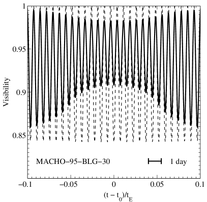
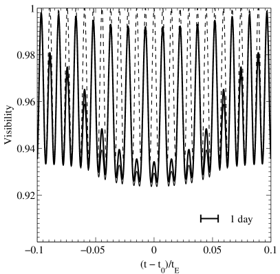
Figure 3: Theoretical visibility measurements for a finite source star with a 2 element interferometer. The separation between interferometer elements is 100m. The wavelength of observation is 2.2 $\mu$m. The event has a declination of $-30^{\circ}$ and the interferometer is at latitude $-40^{\circ}$. The hour angle at maximum lensing amplification is $0.0^{h}$. The event has microlensing parameters similar to the MACHO-95-BLG-30 event, with $u_{\rm min}=0.05408$ and $\rho_{\star}=0.075$. The left and right panels show the visibility with a baseline aligned in the east-west and north-south directions respectively. The visibility for a limb-darkened source and a uniform brightness source is shown by thick and thin lines respectively. The visibility for a point-source is shown by the dashed line.

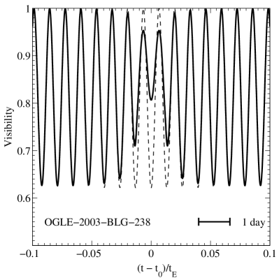
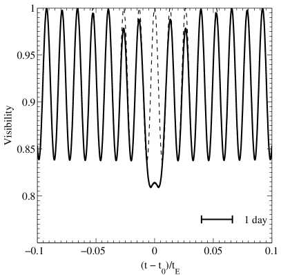
Figure 4: Theoretical visibility measurements for event OGLE-2003-BLG-238. The interferometer parameters are as for Fig. 3, and the event parameters are listed in Table 1.

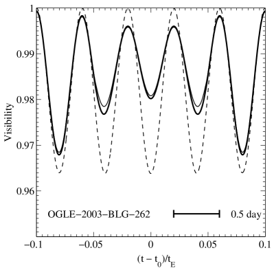
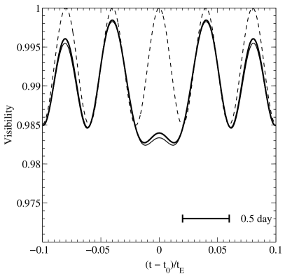
Figure 5: Theoretical visibility measurements for event OGLE-2003-BLG-262. The interferometer parameters are as for Fig. 3, and the event parameters are listed in Table 1.

3.2 Three-element interferometer

We perform the simulations again, using a three-element interferometer with the baselines arranged as an equilateral triangle with baseline length 100m. All other telescope parameters are as above. Figures 6, 7 and 8 show the product of the visibilities from each baseline, $|V_{1}||V_{2}||V_{3}|$, as well as the closure phase for each of the three events listed in Table 1. The source is modelled with limb-darkened and uniform brightness profiles as before. These are compared to the results assuming a point-source. The effect of a finite source star is again evident in the visibility curves around the time of maximum magnification for a time roughly equal to twice the source diameter crossing time. The difference in closure phase due to a finite source exceeds the minimum value detectable by VLTI ($1^{\circ}$) for all events other than OGLE-2003-BLG-238.

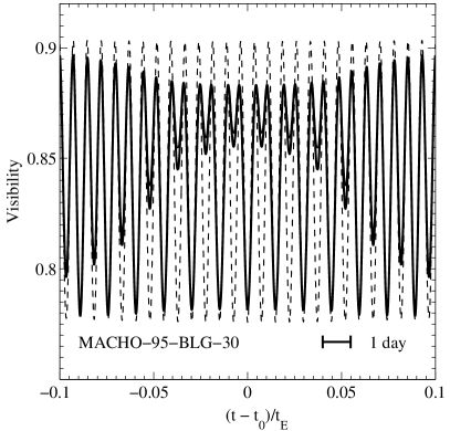
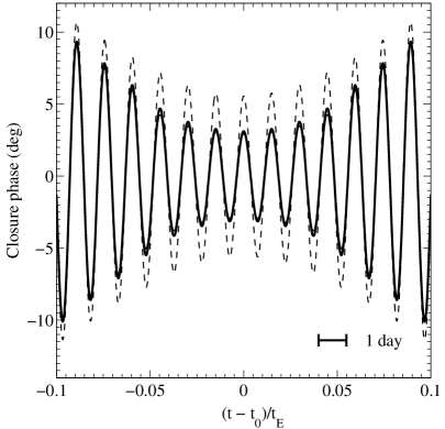
Figure 6: Theoretical measurements using a three-element interferometer for event MACHO-95-BLG-30. The interferometer baselines are arranged as an equilateral triangle with side length $B=100$m. The other interferometer parameters are as given for Fig. 3. The microlensing event parameters are listed in Table 1. Left: The product $|V_{1}|\,|V_{2}|\,|V_{3}|$, see text. Right: The closure phase $(\phi_{12}+\phi_{23}+\phi_{31})$. The results are shown for a limb-darkened source (thick line), uniformly bright source (thin line) and a point source (dashed line).

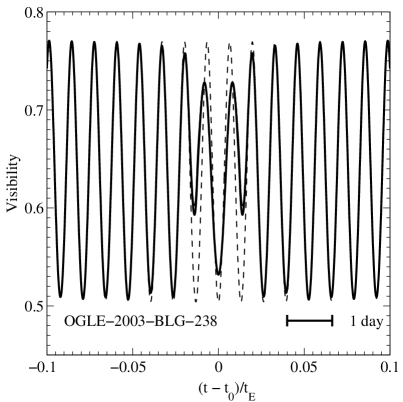
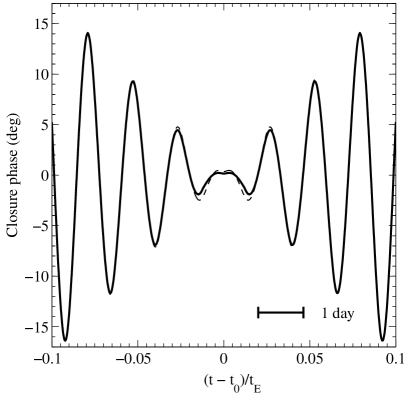
Figure 7: Theoretical measurements using a three-element interferometer for event OGLE-2003-BLG-238. Left: The product $|V_{1}|\,|V_{2}|\,|V_{3}|$, see text. Right: The closure phase. The results are shown for a limb-darkened source (thick line), uniformly bright source (thin line) and a point source (dashed line).

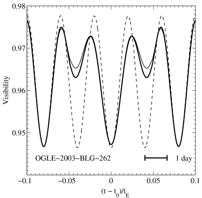
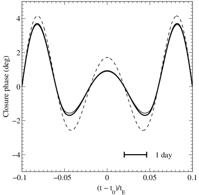
Figure 8: Theoretical measurements using a three-element interferometer for event OGLE-2003-BLG-262. Left: The product $|V_{1}|\,|V_{2}|\,|V_{3}|$, see text. Right: The closure phase. The results are shown for a limb-darkened source (thick line), uniformly bright source (thin line) and a point source (dashed line).

The fraction of microlensing events that will be affected by finite source effects may reach $\sim 3\%$ (1995, see also 1994). The parameters which govern how the visibility and closure phase differs for a finite source with respect to a point source are $\rho_{\star}$ and ${\,u_{\rm min}}$. Figure 9 shows the maximium difference in these observables using a finite source star compared to a point source, as a function of $\rho_{\star}$ and ${\,u_{\rm min}}$. We assume a lens mass of $0.3M_{\odot}$ at a distance 6 kpc, with the source star at 8 kpc. We consider a range of $\rho_{\star}$ corresponding to K and G type giant stars. We note that the maximum difference in visibility due to a finite source star is approximately 13%. The maximum difference in closure phase is approximately 4 degrees. These should be compared with the expected accuracy of the VLTI of $\sim 0.5-5\%$ and $\sim 1^{\circ}$ respectively.

\psfrag{xlabel}{\large\mbox{$\log_{10}(\rho_{\star})$} }\includegraphics[width=218.98021pt]{deltaVis.eps}

\psfrag{xlabel}{\large\mbox{$\log_{10}(\rho_{\star})$} }\includegraphics[width=210.30595pt]{deltaPhi.eps}

Figure 9: The maximum effect of finite source size on visibility and closure phase as a function of source star size, for various values of minimum impact parameter, ${\,u_{\rm min}}$. The parameters of the three-element interferometer are described in the caption of Fig. 6. Left: The fractional change in visibility as a function of the normalised stellar radius, $\rho_{\star}\equiv{\theta_{\rm s}/\theta_{\rm E}}$. The top and bottom solid lines correspond to microlensing events with ${\,u_{\rm min}}=0.001$ and 0.1 respectively. Other values of ${\,u_{\rm min}}$ were used: 0.05 (dashed), 0.02 (dot-dashed), 0.01 (dotted). Right: The absolute change in closure phase owing to finite source effects. The top and bottom lines correspond to ${\,u_{\rm min}}=0.001$ and 0.1 respectively. The approximate source star sizes for K and G type giants at 8 kpc are shown as vertical lines, assuming a 0.3 solar mass lens star at 6 kpc.

4 Summary and Discussion

In this paper, we have studied how the interferometric fringe visibility of a microlensing event is affected by the finite size of the source star. When we take into account realistic telescope sites and interferometer baselines, the visibility undergoes sinusoidal changes, as illustrated in Figures 3–8. Therefore it will be useful to observe the fringe visibilities during multiple epochs for a microlensing event.

We have shown that the fringe visibility can change by as much as $\sim$ 10%, which can be easily measured by the VLTI. Unfortunately, it will be challenging to study limb-darkening profile parameters using interferometers. The ratio $\rho_{\star}=\theta_{\rm s}/\theta_{\rm E}$ can be accurately determined via the modelling of the photometric microlensing light curve. Combined with the source colour, this allows us an approximate determination of the source size, $\theta_{\rm s}$. and thereby the Einstein ring radius $\theta_{\rm E}$. The interferometric finite source size, on the other hand, determines both the angular Einstein radius and the finite source size directly, without reference to the source colour. So the effect of a finite source star size on the fringe visibility complements the photometric finite source size effect. Observations of finite source size events may also be important for another reason: for these events, we already have some indication of the source size, so they can be used to verify the interferometer capabilities, which may be particularly important at early stages.

In addition, the visibility measurement gives us the source trajectory relative to the interferometer baseline. This additional information can be used to further constrain the lens and source kinematics in a maximum likelihood analysis of the lens and source locations.

For a two-element interferometer, when the baseline is perpendicular to the two images, the visibility is always unity so the two micro-images cannot be resolved. This is no longer the case when we have more than two elements, as there are always a baseline that is at some angle to the two micro-images, so the visibility decrement can be observed. Therefore a multiple-element interferometer has a substantial advantage over a two-element interferometer.

The finite source size effect lasts roughly a factor of two times the source diameter crossing time. For the three events listed in Table 1, the source diameter crossing times are about 10, 1 and 1.5 days for MACHO-95-BLG-30, OGLE-2003-BLG-238, and OGLE-2003-BLG-262 respectively, so there should be sufficient time to use interferometers to gain further insights on the lensing parameters. As the finite source size effects can both enhance and decrease the visibility and closure phases, it will be helpful to perform at least two observations: one around the peak of light curve and one shortly afterwards when the finite source size effect is no longer important.

In this paper, we have not studied binary lensing events under either a point source approximation or with realistic finite source sizes. Some of these events will have large magnifications during a caustic crossing. It will be interesting to study the interferometric signals of this class of events, and how the visibility changes during a binary (including planetary) lensing event, and what extra information one can extract.

We thank Ian Browne and Neal Jackson for many helpful discussions about interferometry; Bohdan Paczyński, Duncan Lorimer, Andrea Richichi, Phil Yock and the referee for their comments on this manuscript. NJR is supported a PPARC postdoctoral grant. This work was partially supported by the European Community’s Sixth Framework Marie Curie Research Training Network Programme, Contract No. MRTN-CT-2004-505183 ‘ANGLES’.

Appendix A Fringe Visibility when the source is exactly along the line of sight

When the source is exactly aligned with the line of sight, the images form an annulus. The inner and outer radii in units of the Einstein radius are given by

$$r_{+,-}={\sqrt{\rho_{\star}^{2}+4}\pm\rho_{\star}\over 2},$$ (18)

where $\rho_{\star}$ is the physical source size in units of the Einstein radius.

To derive the visibility, it is natural to use the cylindrical coordinate system due to symmetry. Without losing generality, we can put the interferometer baseline along the horizontal axis. Let us assume the source has uniform surface brightness. Recall that $\vec{\cal K}_{\rm cr}\cdot\vec{r}={{\cal K}_{\rm cr}}r\cos\theta$, where $\theta$ is the polar angle, and ${{\cal K}_{\rm cr}}=2\pi B\theta_{\rm E}/\lambda$. The complex visibility is given by

$$\hat{V}={1\over\int_{r_{-}}^{r_{+}}2\pi rdr}\int_{r_{-}}^{r_{+}}rdr\int_{0}^{2\pi}\exp(i{{\cal K}_{\rm cr}}r\cos\theta)d\theta=2\,{r_{+}J_{1}({{\cal K}_{\rm cr}}r_{+})-r_{-}J_{1}({{\cal K}_{\rm cr}}r_{-})\over{{\cal K}_{\rm cr}}(r_{+}^{2}-r_{-}^{2})},$$ (19)

where $J_{n}(x)$ is the usual Bessel function of order $n$. Notice that due to symmetry, the visibility $\hat{V}({{\cal K}_{\rm cr}})$ is real.

For an infinitesimal source, i.e., at the limit $\rho_{\star}\rightarrow 0$, we find

$$\hat{V}={J_{1}({{\cal K}_{\rm cr}})\over{{{\cal K}_{\rm cr}}}}+{J_{0}({{\cal K}_{\rm cr}})-J_{2}({{\cal K}_{\rm cr}})\over 2}.$$ (20)

References

- Abe et al. (2003) Abe F. et al., 2003, A&A, 411, L493
- Albrow et al. (1999) Albrow M. et al., 1999, ApJ, 522, 1011
- Albrow et al. (2001) Albrow M. et al., 2001, ApJ, 549, 759
- Alcock et al. (1997) Alcock C. et al., 1997, ApJ, 491, 436
- Allen (1973) Allen C. W., 1973, Astrophysical Quantities. Athone Press, London, p. 170
- An et al. (2002) An J. H. et al., 2002, ApJ, 572, 521
- Burke & Graham-Smith (2002) Burke B. F., Graham-Smith F., 2002, An Introduction to Radio Astronomy 2nd ed. Cambridge University Press, Cambridge
- (8) Castro S., Pogge R. W., Rich R. M., DePoy D. L., Gould A., 2001,ApJ, 548, L197
- (9) Cornwell T. J., Wilkinson P. N., 2001, ApJ, 548, L197
- Claret et al. (1995) Claret A., Díaz-Coroveś J., & Gimémez A., 1995, A&AS, 114, 247
- (11) Dalal N., Lane J., 2003, ApJ, 589, 199
- (12) Delplancke F., Górski K. M., Richichi A., 2001, A&A, 375, 701
- (13) Gould A., 1992, ApJ, 392, 442
- (14) Gould A., 1994, ApJ, 421, L71
- (15) Høg E., Novikov I. D., & Polnarev A. G., 1995, A&A, 294, 287
- Hosokawa et al. (1993) Hosokawa M., Ohnishi K., Fukushima T., & Takeuti M., 1993, A&A, 278, L27
- Jennison (1958) Jennison R. C., 1958, MNRAS, 118, 276
- (18) Jiang G. F. et al., 2004, ApJ, 617, 1307
- Liebes (1964) Liebes S., 1964, Phys Rev B, 133, 835
- (20) Mao S., Witt H. J., 1998, MNRAS, 300, 1041
- (21) Miralda-Escudé J., 1996, ApJ, 470, L113
- Miyamoto & Yoshi (1995) Miyamoto M. & Yoshi Y., 1995, AJ, 110, 1427
- Nemiroff & Wickramasinghe (1994) Nemiroff R. J., Wickramasinghe W. A. D. T., 1994, ApJ, 424, L21
- (24) Paczyński B., 1996, ARA&A, 34, 419
- (25) Paczyński B., 1998, ApJ, 494, L23
- Shao (2004) Shao, M., 2004, “Science overview and status of the SIM project”, in New Frontiers in Stellar Interferometry, Proceedings of SPIE Volume 5491. Edited by Wesley A. Traub. Bellingham, WA: The International Society for Optical Engineering, 2004., p.328
- (27) Rattenbury N. J., et al., 2005, A&A, 439, 645-650
- ten Brummelaar et al. (2005) ten Brummelaar, T. A., 2005 ApJ, 638, 453-465
- Mariotti (1998) Mariotti, J.-M. et al, 1998, SPIE’s International Symposium on Astronomical Telescopes and Instrumentation, Conf. 3350 “Astronomical Interferometry”, Hawaii, USA
- Booth (1999) Booth, A. J. et al, 1999, “The Keck Interferometer: Instrument Overview and Proposed Science”, in ASP Conf. Ser. 194: Working on the Fringe: Optical and IR Interferometry from Ground and Space
- Perryman (2005) Perryman, M. A. C., 2005, “Overview of the Gaia Mission”, in ESA SP-576: The Three-Dimensional Universe with Gaia
- Thompson et al. (2001) Thompson A. R., Moran J. M., Swenson G.W., 2001, Interferometry and Synthesis in Radio Astronomy 2nd ed. Wiley-Interscience, New York
- (33) Walker M. A., 1995, ApJ, 453, 37
- (34) Witt H. J., 1990, A&A, 236, 311
- (35) Witt H. J., Mao S., 1994, ApJ, 430, 505
- (36) Witt H. J., 1995, ApJ, 449, 42
- Yoo et al. (2004) Yoo J. et al., 2004, ApJ, 603, 139